3 Vector Quantization. 6. 3.1 Quantization Error of Vector Quantizers . . . . . . . . . . . . 7. 3.2 Optimality Conditions for Vector Quantizers . . . . . . . . . 8.
ARMY RESEARCH LABORATORY
Video Compression using Vector Quantization by Mahesh Venkatraman, Heesung Kwon, and Nasser M. Nasrabadi
ARL-TR-1535
May 1998
19980519 086 DnC QUALITY INSPECTED 3 Approved for public release; distribution unlimited.
The findings in this report are not to be construed as an official Department of the Army position unless so designated by other authorized documents. Citation of manufacturer's or trade names does not constitute an official endorsement or approval of the use thereof. Destroy this report when it is no longer needed. Do not return it to the originator.
Army Research Laboratory Adelphi, MD 20783-1197 ARL-TR-1535
May 1998
Video Compression using Vector Quantization Mahesh Venkatraman, Heesung Kwon, and Nasser M. Nasrabadi Sensors and Electron Devices Directorate
Approved for public release; distribution unlimited.
Abstract
This report presents some results and findings of our work on very-lowbit-rate video compression systems using vector quantization (VQ). We have identified multiscale segmentation and variable-rate coding as two important concepts whose effective use can lead to superior compression performance. Two VQ algorithms that attempt to use these two aspects are presented: one based on residual vector quantization and the other on quadtree vector quantization. Residual vector quantization is a successive approximation quantizer technique and is ideal for variable-rate coding. Quadtree vector quantization is inherently a multiscale coding method. The report presents the general theoretical formulation of these algorithms, as well as quantitative performance of sample implementations.
11
Contents
1 Introduction: Very-Low-Bit-Rate Video Coding for the Digital Battlefield
1
2 Background
3
2.1
Quantization
3
2.2 Video Compression
4
2.3 Motion Compensation . .
4
3 Vector Quantization 3.1
6
Quantization Error of Vector Quantizers
7
3.2 Optimality Conditions for Vector Quantizers
8
3.2.1
Nearest-Neighbor Condition
8
3.2.2
Centroid Condition
8
3.3 Design of Vector Quantizers 3.3.1
Generalized Lloyd's Algorithm
3.3.2
Kohonen's Self-Organizing Feature Map
9 9 10
3.4 Entropy-Constrained Vector Quantizer
10
3.5 Video Compression Using Vector Quantization
11
4 Residual Vector Quantization 4.1
13
Residual Quantization
13
4.2 Residual Vector Quantizer
14
4.3 Search Techniques for Residual Vector Quantizers
14
4.3.1
Exhaustive Search
15
4.3.2
Sequential Search
15
4.3.3
M-Search
15
4.4 Structure of Residual VQs
15 m
4.5 Optimality Conditions for Residual Quantizers 4.5.1
Overall Optimality
16
4.5.2
Causal Stages Optimality
17
4.5.3
Simultaneous Causal and Overall Optimality
18
4.6 Design of Residual Vector Quantizers
19
4.7 Residual Vector Quantization with Variable Block Size ....
19
4.8 Pruned Variable-Block-Size Residual Vector Quantizer. ...
19
4.8.1
Top-Down Pruning Using a Predefined Threshold . .
20
4.8.2
Optimal Pruning in the Rate-Distortion Sense ....
20
4.9 Transform-Domain Vector Quantization for Large Blocks . .
20
4.10 Video Compression Using Residual Vector Quantization . .
21
4.10.1 Theory of Residual Vector Quantization
21
4.10.2 Performance of an RVQ-Based Video Codec
24
5 Quadtree-Based Vector Quantization 5.1
IV
16
Quadtree Decomposition
30 30
5.2 Optimal Quadtree in the Rate-Distortion Sense
31
5.3 Video Compression Using Quadtree-Based Vector Quantization
32
6 Conclusions
33
References
34
Distribution
37
Report Documentation Page
41
Figures
1
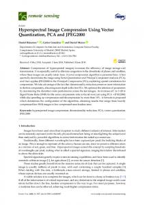
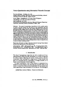
Original and compressed representations of a frame from a FLIR video sequence
2
2
Scalar quantizer Q of a random variable Xn
4
3
Motion compensation for video coding
4
Entropy of a sequence after decorrelation in temporal dimension
5
5
Encoder/decoder model of a VQ
7
6
Entropy coding of VQ indices
10
7
VQ encoder for two-dimensional arrays
11
8
VQ decoder for two-dimensional arrays
12
9
Residual quantizer—cascade of two quantizers
14
10
Structure of a residual VQ
16
11
Tree structure of variable-block-size residual VQ
19
12
Optimal pruning of residual VQ in rate-distortion sense ...
21
13
Video encoder based on residual vector quantization ....
22
14
Video decoder based on residual vector quantization ....
23
15
Performance of video compression algorithms using vector quantization
26
16
Results for bit rate of approximately 12 kb/s
27
17
Results for bit rate of approximately 8.1 kb/s
28
18
Results for bit rate of approximately 5.3 kb/s
29
19
Vector quantization of quadtree leaf nodes
31
20
Encoding quadtree data structure
32
5
1. Introduction: Very-Low-Bit-Rate Video Coding for the Digital Battlefield
Battlefield digitization—the process of representing all components of a battlefield in digital form—allows the battlefield and its components to be visualized, simulated, and processed on computer systems, making the Army more deadly and reducing the use of physical resources. For complete battlefield digitization, images of various modalities must be gathered by different imaging techniques. These images are then processed to provide important information about the imaged areas. An important class of visual data is the image sequence or video, and forward-looking infrared (FLIR) video is an important source of information. These data consist of a series of two-dimensional images captured at a constant temporal rate. The main drawback to effective use of this data source is the huge amount of raw digital data (bits) required to represent them. This volume of data makes real-time gathering and transmission over tactical internets impractical. To effectively combat this problem, data compression is used: that is, techniques to reduce the number of bits required to represent the data. The large compression ratios needed to "squeeze" video over low-bandwidth digital channels require the use of "lossy" image compression techniques. Lossy compression techniques use a very small number of bits to represent the data at the cost of degraded information. These techniques require a trade-off between video quality and bit-rate constraints. For intelligent compression of FLIR video images, the bit assignment should be made so that more bits are assigned to active areas, while fewer are assigned to passive background areas. Vector quantization (a block quantization technique) has this type of adaptability, so that it is highly suitable for compressing FLIR video. In the work reported here, we systematically study the use of vector quantization for compressing video sequences. Results are shown for both FLIR video and regular gray-scale video. (A single representative frame of the original FLIR video scene and its compressed representation are shown in fig. 1.) We specifically study two adaptive vector quantization techniques: the residual vector quantizer (VQ) and the quadtree VQ. These two techniques permit the encoding of sources at different levels of precision depending on content.
Figure 1. Original (top) and compressed (bottom) representations of a frame from a FLIR video sequence.
The targeted bit rate is in the very low (5 to 16 kb/s) range; this rate allows the compressed video to be transmitted over SINCGARS (Single-Channel Ground to Air Radio System) channels, as well as permitting multiple video streams to be multiplexed and transmitted over Fractional Tl lines. Such multiplex transmission would allow the video to be collected by sources such as unmanned airborne vehicles (UAVs) and transmitted to processing centers in real time.
2. Background
Images are represented in the digital domain by a matrix/array of intensity values, and video sequences are represented by a series of matrices. These matrices are often large, requiring large amounts of storage space and/or transmission bandwidth. When resources are limited (storage spaces or bandwidth), it is essential to reduce the amount of data necessary for representing the digital imagery. Data can be reduced (compressed) either with no loss in data (lossless compression) or with some degradation/distortion of the data (lossy compression). In lossless compression, redundancy in the data is removed, resulting in a smaller representation, but the ratio of compression that can be achieved is small. On the other hand, lossy compression techniques trade off the compression ratio against the tolerated distortion. Most current image- and video-compression techniques are lossy, since human visual perception can tolerate a certain amount of distortion in the presented visual data. Lossy compression can be achieved by quantization, a lossy compression technique in which data are represented at lower numerical precision than in the original representation. 2.1
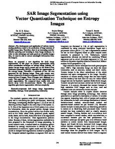
Quantization A quantization Q of a random variable X e TZ is a mapping from 1Z to C, a finite subset of TZ: Q : TZ H-» C, C C TZ. (1) The cardinality Nc of the set C gives the number of quantization levels. The mapping Q is generally a staircase function, as shown in figure 2, where TZ is divided into Nc segments [bi — 1,bt),i = l,...,N. EachXn € [6j - 1,h) is mapped to c* € C, where Cj is the reconstruction value. A sequence of random variables Xn can be quantized by two different methods. The first method involves each individual member of the sequence being quantized separately by the quantizer Q defined above. This method is called scalar quantization. In the second method, the sequence is grouped into blocks of adjacent members, and each block (a vector) is quantized by a vector quantizer. In the work reported here, vector quantization (sect. 3) is applied to video compression.
n ■-C„-2 -■c„-i V-3 H
b„-2 1
fc«-1
-- C„-2
Figure 2. Scalar quantizer Q of a random variable Xn.
2.2
Video Compression A video sequence is a three-dimensional signal of light intensity, with two spatial dimensions and a temporal dimension. A digital video sequence is a three-dimensional signal that is suitably sampled in all three dimensions; it is in the form of a three-dimensional matrix of intensity values. A typical video sequence has a significant amount of correlation between neighbors in all three dimensions. The type of correlation in the temporal dimension is significantly different from that in the spatial dimensions. There are many different approaches to video compression, and some international compression standards have been established. Among the different approaches is a class of algorithms that first attempt to remove correlations in the temporal domain and then deal with removing correlations in the spatial dimensions. Among these is motion compensation (MC), a popular technique to remove the correlations in the temporal domain. Motion compensation results in a residue sequence, which is then quantized by two-dimensional quantization techniques similar to those used for compressing still images.
2.3
Motion Compensation A video scene usually contains some motion of objects, occlusion/exposure of areas due to such motion, and some deformation. The rate of these changes is typically much smaller than the frame rate (i.e., the rate of sampling in the temporal dimension). Therefore, there is very little change between two adjacent frames. A motion-compensation algorithm exploits this consistency to approximate the current frame by using pieces from the previous frame. The result is a reasonable approximation of the current frame based on the previous one, with some side information in the form of motion vectors. The difference between the approximation of the current frame and the actual frame is quantized by a set of scalar or vector quantizers.
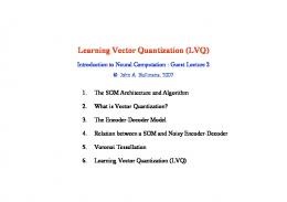
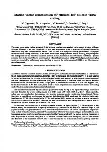
In figure 3, which shows the block diagram of the encoder and decoder, the difference between the approximation and the original is quantized by the quantizer Q. The encoder is a closed-loop system, as shown in the block diagram; it contains both a quantizer Q and an inverse quantizer Q~x. Since the encoder uses the previous frame to approximate the current frame, the decoder needs the previous frame to generate the current frame. The decoder has only the quantized version of the previous frame and not the original frame. The inverse quantizer Q-1 in the encoder duplicates the decoder states at the encoder and gives the encoder access to a quantized version of the previous frame. The encoder uses this quantized version of the previous frame to generate an approximation of the current frame. This ensures that the approximation of the current frame generated from the previous frame is the same at both the encoder and decoder. Figure 4 shows the entropy of a sequence after (1) decorrelation by taking the frame difference and (2) decorrelation using block motion estimation. It can be seen that the entropy in this case is reduced by a factor of two compared to the original frame entropy. Between frames 105 and 120, the entropy of the residue due to motion estimation is significantly less than the entropy of the residue from frame differencing. This difference is due to significant motion of objects in the images during that period. Decoder
Encoder
t
(MCJ-^Dejay) (Delay)
HMCh*
Figure 3. Motion compensation (MC) for video coding.
Decorrelation using frame difference Decorrelation using block motion estimation Original frames
0
15
30
45
60 75 90 Frame number
105
120
135
Figure 4. Entropy of a sequence after decorrelation in temporal dimension.
3. Vector Quantization
A vector quantizer Q is a mapping from a point in fc-dimensional Euclidean space Tlk into a finite subset C of Tlk containing N reproduction points or vectors: Q : TZk ■-> C.
The N reproduction vectors are called codevectors, and the set C is called the codebook. C = (ci, c2,..., cn), and Cj 6 Tlk for each i e T = {1,2,..., N}. The codebook C has JV distinct members. The rate of the VQ, r = log2(N), measures the number of bits required to index a member of the codebook. A VQ partitions the space Tlk into cells 7^: Tli = {X € Tlk : Q(X) = Ci}Vi € T. These cells represent the pre-image of the points c* under the mapping Q, i.e., Tli = = E(d(X,Q(X))), where d(X, Q(X)) represents the distortion introduced by the quantizer for the input vector X. One important distortion measure is the squared-error distortion measure (Euclidean distortion/L^ distortion). This distortion measure is especially relevant to image coding problems, where the mean squared error is widely used as a quantitative measure of the performance of coding: d(X,Q(X))' = ||X-Q(X)||2, V = E(||X-Q(X)||2). Other distortion measures include the weighed squared-error distortion measure, the Mahalanobis distortion measure, and the Itakura-Saito distortion measure.
3.2
Optimality Conditions for Vector Quantizers An optimal VQ is one that minimizes the overall distortion measure for any vector X with a probability distribution P(X). A VQ has to satisfy two optimality conditions to achieve this minimum distortion: • For a given fixed decoder ß, the encoder 7 should be the one that minimizes the overall distortion. • For a given fixed encoder 7, the decoder ß should be the best possible decoder.
3.2.1 Nearest-Neighbor Condition Given a decoder, it is necessary to find the best possible encoder. The decoder contains a finite set of vectors C, one of which is used to represent the input vector. For a given vector X, the vector Cj is the nearest neighbor if d(X, cj) < d(X, cj)
V cj € C.
The overall distortion for a given fixed codebook C is given by 2> = E(d(X,Q(X))),
V = Jd(X,Q(X))P(X)dX; clearly,
J d(X, Q(X))P(X) dX > J d(X, Ci)P(X) dX, where c* is the nearest neighbor of X. Therefore, the best possible encoder for a given decoder is the nearest-neighbor encoder. 3.2.2 Centroid Condition For a fixed encoder, it is necessary to find the reproduction codebook that minimizes the overall distortion. For a given cell TU, the centroid Cj is defined as
2>(x, Ci) < p(x, c) v x, c G Hi, a e
TU.
For a given probability distribution, and for a given encoder, the overall distortion is given by 2> = |d(X,Q(X))P(X)dX,
2> = W d(X,c)P(X)dX.
Clearly,
W d(X,c)P(X)dX> J2 I d(X,Ci)P(X)dX. Therefore, for a given encoder, the optimum decoder is the centroid of the nearest-neighbor partitions. Consider the set A of all possible partitions of the input vectors, and a collection C° of all possible reproduction sets. The optimum VQ is the pair ({Ki},C);{Ri}e A andCeC°, such that Hi is the nearest neighbor partition of C that contains the centroids of the partitions in Hi. These two conditions are generalizations of the Lloyd-Max conditions for scalar quantizers. 3.3
Design of Vector Quantizers Design of VQs is a very difficult problem. For a given probability distribution P(X), it is necessary to find the encoder and decoder that simultaneously satisfy both the nearest-neighbor condition and the centroid condition. Unfortunately, no closed-form solutions exist for even simple distributions. A number of methods have been proposed for the design of VQs. All these are iterative methods based on finding the best VQ for a training set.
3.3.1 Generalized Lloyd's Algorithm The generalized Lloyd's algorithm (GLA) (also known as the LBG algorithm after Linde, Buzo, and Gray [1]) is an iterative algorithm. This algorithm, which is similar to the fc-means clustering algorithm, consists of two basic steps: • For a given codebook Ct, find the best partition {Tli}t of the training set satisfying the nearest-neighbor neighborhood condition. • For the new partition {Tli}t, find the best reproduction codebook Ct+i satisfying the centroid condition. These two steps are repeated until the required codebook is obtained. The training algorithm begins with an initial codebook, which is refined by the Lloyd's iterations until an acceptable codebook is obtained. A codebook is considered acceptable if the error difference between the present and the previous codebooks is less than a threshold.
3.3.2 Kohonen's Self-Organizing Feature Map Kohonen's self-organizing feature maps (KSOFMs) can be used to design VQs with optimal codebooks [2,3]. In this method of codebook design, an energy function for error is formulated and minimized iteratively. This design procedure is sequential, unlike GLA, which uses the batch method of training. 3.4
Entropy-Constrained Vector Quantizer For transmission over a binary channel, the index of the reproduction vector from a codebook C of size N is represented by a binary string of length |"log2 N] bits. Often, it is possible to further reduce the number of bits required to represent the indices by using entropy coding as shown in figure 6. Entropy coding reduces the transmission entropy rate from [log2 N) per block to almost the entropy rate of the index sequence. Since typical codebook design algorithms do not consider the possible entropy rates of the index sequences, the codebooks do not combine with an entropy coder in an optimal way. Design of entropy-constrained VQs (ECVQs) has been studied by Chou et al [4] (among others), who used a Lagrangian formulation with a gradient-based algorithm similar to the Lloyd's algorithm to design the codebooks. Consider a vector X e Tlk quantized by a VQ with a codebook C = {c, : j = 1,..., N}. Let l(i) represent the length of the binary string used to represent the index i of the reproduction vector c^ of X. Then the energy function that is minimized in the design of an ECVQ is given by [4] J(7,/?) = E[d(xi,Q(xi)] + XE[l(t)},
(2)
where 7 and ß are the VQ encoder and decoder, respectively. The index entropy log(l/p(i)) is used in the algorithm to represent the length of the binary string required to represent the index i. The codebook is then designed x Input vector
ß(X) Approx. of input vector
Encoder Y
Decoder
ß
Entropy encoder
Entropy decoder
Figure 6. Entropy coding of VQ indices.
10
in an iterative manner, similar to the Lloyd's algorithm, through choosing an encoder and decoder that decrease the energy function in equation (2) at every iteration. Experimental results have shown that the ECVQ design algorithm described above gives an encoder-decoder pair that has superior numerical performance. 3.5
Video Compression Using Vector Quantization The residual signal obtained after motion compensation can be compressed by vector quantization. The two-dimensional signal is divided into blocks of equal size, as shown in figure 7. The VQ encoder that is used to compress the residual signal is a nearest-neighbor encoder. It has a reference lookup table that contains the centroids of the VQ partitions. The encoder compares each block (in some predefined scanning order) with each member of the lookup table to find the closest match in terms of the defined distortion measure (usually the mean-squared error). The index of the closest matching codevector in the lookup table is then transmitted/stored as the compressed representation of the corresponding vector (block). The decoder is a simple lookup table decoder, as shown in figure 8. The decoder uses the index symbol generated by the encoder as a reference to an entry in a lookup table in the decoder. The lookup table in the decoder is usually identical to the one in the encoder. This lookup table contains the possible approximations for the blocks in the reconstructed image. Based on the index, the approximate representation of the current block is determined. To generate the reconstructed two-dimensional array, the decoder places this representation at the position corresponding to the scanning order. The reconstructed array is used along with the motion-compensation algorithm to reproduce the compressed video sequence. • • • •
• • • •
• • • •
• • • •
Nearestneighbor encoder Y
_ Channel symbol
Image divided into blocks
Lookup table
Figure 7. VQ encoder for two-dimensional arrays.
11
• • • • Channel symbol
^-
Table lookup decoder
ß
• • • • • • • •
t
• ••• • ••• • •••
Reconstructed image
Lookup table
Figure 8. VQ decoder for two-dimensional arrays.
12
4. Residual Vector Quantization
Residual vector quantization (RVQ) is a structured vector quantization scheme proposed mainly to overcome the search and storage complexities of regular VQs [5,6]. Residual VQs are also known as multistage VQs. They consist of a number of cascaded VQs. Each stage has a VQ with a small codebook that quantizes the error signal from the previous stage. Residual quantizers are successive-refinement quantizers, where the information to be transmitted/stored is first approximated coarsely and then refined in the successive stages. 4.1
Residual Quantization Consider a random variable X with a probability distribution function P(X). Let Q1{X) be an N1 level quantizer and its associated bit rate be log2(AT1) bits. The error due to this quantizer is R1 = X1 - Q V), and the expected value of the distortion is given by Vl= fd{X\Q1(Xl))P{X1)dX1. If the random variable needs to be represented more precisely (i.e., if the expected value of the distortion needs to be smaller), the first-stage residue can be quantized again by a second quantizer Q2. The quantizer Q2 approximates the random variable Rl. Let Q2(i?1) be an N2 level quantizer, and its associated bit rate be log2(7V2) bits. The error due to this quantizer is given by R2 = R1- Q2(R1), and the expected value of distortion is now
V2 = J d[X, (Q^X) + Q2(R1))]P(X) dX. This process can be thought of as a cascade of two quantizers, as shown in figure 9. The total bit rate of the quantization scheme is log2(AT1)+log2(iV2).
13
1
Q
1 Q1(x).
Q2(/?1)
Figure 9. Residual quantizer—cascade of two quantizers.
This scheme can be extended to any number of quantizers. A if-stage residual quantizer consists of K quantizers {Qfc : k = 1,..., K}. Each quantizer Qfc quantizes the residue of the previous stage, i?(fc_1). The total bit rate of the quantization scheme is given by
B = 5>g2(iV*), fc=0
where Nk is the number of quantization levels of the quantizer Qk. 4.2
Residual Vector Quantizer A residual VQ is a vector generalization of the residual quantizer outlined above. A if-stage residual VQ is composed of K VQs {Qfc : k = 1,..., K). Each VQ consists of its own codebook Ck of size Nk. The fcth-stage VQ operates on the residue R(fc_1) from the previous stage. The residue due to the first stage is given by R^X-Q^X). The final quantized value of the vector X is given by Q(X) = QX(X) + Q^R1) + ... + Q^R^"1)) + ... + Q^R^-D).
4.3
Search Techniques for Residual Vector Quantizers The structure of a residual VQ inherently lends itself to a number of possible encoding schemes. Two of the main characteristics of encoding in residual quantizers are • overall optimality—the least overall distortion at the end of the last stage of encoding, and • stage-wise optimality—the least distortion possible at the end of each stage.
14
4.3.1 Exhaustive Search Exhaustive search in residual quantizers aims at achieving the least overall distortion. In exhaustive search schemes, all possible combinations of all the stage quantizations are searched, and the combination giving rise to the least distortion is chosen. This search gives the best possible performance in the residual quantization scheme. But this search scheme is computationally very expensive and is the same as that of an unstructured VQ. The search complexity for a K-siage VQ with codebook sizes {Ni, N2,... NK} is of the order 0(N\ x iV2 x ... Afc). Exhaustive search schemes are not particularly appropriate for progressive transmission schemes (successive refinement). 4.3.2 Sequential Search Sequential search in residual quantizers makes full use of the structural constraint of the quantizer. The search process is stage by stage, wherein the quantization value that minimizes the distortion up to that stage is chosen. This search scheme is inherently inferior to exhaustive schemes, leading usually to suboptimal overall distortion performance. It is also the least expensive of all search schemes. The search complexity for a If-stage quantizer with codebook sizes {Ni, N2,... NK} is of the order 0(Ni + N2 + ... NK)- The search scheme is particularly well-suited for progressive transmission schemes. 4.3.3 M-Search A hybrid search scheme, M-search, has been proposed [7] whose search complexity is less than that of a full search, but greater than that of a sequential. This scheme produces overall distortion performance that is better than that of sequential search schemes and close to that of the exhaustive search scheme. In this scheme, a subset of the quantization values is chosen at each stage based on the least distortion; these subsets are searched in an exhaustive fashion to get the quantized value. 4.4
Structure of Residual VQs A quantizer partitions an input space into a finite number of polytopal regions (fig. 10). The centroid of each polytope approximates all the input symbols that belong to that particular region. The process of finding the residue of the signal is equivalent to shifting the coordinate system to the centroid of the polytope. This process is repeated for all the polytopes. Therefore, we have a finite set of spaces, each corresponding to a polytope. These spaces are bounded by the underlying polytope of the partition; i.e., 15
* Polytopes of firststage VQ
Shifting coordinates (residue)
Joint partition of two stages
Tree-structured vector quantizer
Second-stage partition
Residual vector quantizer
Figure 10. Structure of a residual VQ.
each of these spaces contains members around the origin that are limited in location by the polytope to which they belong. Now consider the quantization of each of these spaces. If the optimal quantizer is found for each of these spaces, their structures (i.e., the partition of the input space) may be totally different. Such a quantizer is called a treestructured quantizer. If a constraint is imposed such that the same partition structure is used for all the subspaces, then the method of quantization is the residual quantization scheme. 4.5
Optimality Conditions for Residual Quantizers
4.5.1 Overall Optimality Consider a if-stage residual quantizer with a set of quantizers Q, Q = {Q\Q2,...,Qk,...Qn} and codebooks C, C = {C\C2,...,Cfe,...Cn}, with stage indices K = {k : k = 1... K}. Each stage codebook Ck contains Nk codevectors Ck = {cj, c|,..., c^fc}. As with VQs, we derive two optimality conditions. For the first condition, given the encoder, we find the best possible decoder. For the second condition, we find the best possible 16
encoder for a given decoder. We derive the conditions for a particular stage, assuming that all other stages have fixed encoders and decoders. Centroid condition: The index vector I belongs to the index space J = {I : I = (i1, i2,..., ik,... iK), ik = 1,..., Nk}. Let the partition of the input space be Vi = V„i „2 „fc „K , based on the different stage quantizers. This partition is based on a fixed encoder. To find the best decoder for the stage K, let the decoders of stages {K|K} be fixed. Overall distortion is given by
2>(X, Q(X)) = £ £(X - 4 " 4 • • • " cJT-\ ~