Addition spectrum, persistent current, and spin polarization in coupled

Addition spectrum, persistent current, and spin polarization in

arXiv:cond-mat/9802057v1 [cond-mat.mes-hall] 4 Feb 1998

coupled quantum dot arrays: coherence, correlation, and disorder R. Kotlyar, C. A. Stafford,∗ and S. Das Sarma Department of Physics, University of Maryland, College Park, MD 20742-4111, USA (February 1, 2008)

Abstract The ground state persistent current and electron addition spectrum in twodimensional quantum dot arrays and one-dimensional quantum dot rings, pierced by an external magnetic flux, are investigated using the extended Hubbard model. The collective multidot problem is shown to map exactly into the strong field noninteracting finite-size Hofstadter butterfly problem at the spin polarization transition. The finite size Hofstadter problem is discussed, and an analytical solution for limiting values of flux is obtained. In weak fields we predict novel flux periodic oscillations in the spin component along the quantization axis with a periodicity given by ν h/e (ν ≤ 1). The sensitivity of the calculated persistent current to interaction and disorder is shown to reflect the intricacies of various Mott-Hubbard quantum phase transitions in two- dimensional systems: the persistent current is suppressed in the antiferromagnetic Mott-insulating phase governed by intradot Coulomb interactions; the persistent current is maximized at the spin density wave - charge density wave transition driven by the nearest neighbor interdot interaction; the Mott-insulating phase persistent current is enhanced by the long-range

∗ Current

and Permanent address: Fakult¨at f¨ ur Physik, Albert-Ludwigs-Universit¨ at, D-79104

Freiburg, Germany.

1

interdot interactions to its noninteracting value; the strong suppression of the noninteracting current in the presence of random disorder is seen only at large disorder strengths; at half filling even a relatively weak intradot Coulomb interaction enhances the disordered noninteracting system persistent current; in general, the suppression of the persistent current by disorder is less significant in the presence of the long-range interdot Coulomb interaction. PACS numbers: 73.20.Dx, 73.23.Hk, 71.10.Fd

Typeset using REVTEX 2

I. INTRODUCTION

In this paper we consider an array of coherently coupled1–5 semiconductor quantum dots arranged in finite two-dimensional (2D) square lattices or one-dimensional (1D) rings pierced by a magnetic flux oriented normal to the lattice or the ring plane. At low temperatures, these quantum dot arrays may be considered “artificial molecules” (with individual quantum dots being the “atomic” constituents of these artificial molecules) because the electron phase coherence length is comparable to the array linear size. Theoretical work on multidot systems has mostly concentrated on the two limiting situations: coherent dots with no Coulomb interaction6 and Coulomb blockade of individual dots7,8 . In this paper, we consider quantum dot arrays taking into account quantum fluctuations arising from interdot hopping, electron-electron interaction, and random disorder effects through an extended Hubbard-type Hamiltonian9–11 In a previous paper,11 we reported on our prediction of an equilibrium persistent current in finite 2D dot arrays (without any periodic boundary conditions) in the presence of an applied magnetic field transverse to the 2D plane. In this paper we provide details and expand on our previous work, and present results for the electron addition spectrum and the persistent current in 2D square lattices and 1D rings including effects of collective physics arising from the multiple dot structure of the system within a simple model for the singleparticle physics12 of the individual quantum dots. One of our primary motivations is to understand lattice effects on the persistent current and the electron addition spectrum, the lattice here being the artificial lattice defining the 2D or the 1D quantum dot array (with the typical lattice constant in the 20 − 200 nm range). One goal is to identify experimentally observable features of various Mott-Hubbard quantum phase transitions (including realistic disorder and interaction effects) in semiconductor quantum dot arrays. The importance of electron-electron interaction has been stressed13–18 in the literature in the context of persistent current experiments in 1D gold and semiconductor rings4 . The magnitude of the persistent current4 in disordered gold rings was found to be one to two 3

orders of magnitude larger than that theoretically predicted, whereas in clean semiconductor rings the magnitude of the persistent current was found to be in a good agreement with the theoretically predicted simple noninteracting value of e vF /L (with vF being the Fermi velocity of electrons moving in a ring of length L, in our notation L denotes the size of the system as defined by the total number of dots in it). Although the interplay between disorder and Coulomb interaction in determining the magnitude of the persistent current in ring topologies is the subject of many recent theoretical investigations16,17,19 , the issue remains unsettled. Disorder and interaction effects are naturally included in our MottHubbard model of finite quantum dot arrays, and we will comment on their influence on the persistent current. The paper is organized as follows. In Sec. II we define and describe the extended MottHubbard Hamiltonian9 which forms the basis of our theoretical description of the collective physics in finite quantum dot lattices. In Sec. III we present our calculated electron addition spectrum as a function of the externally applied magnetic flux for a 3 × 3 lattice and an L = 9−site ring, and identify the main features of these results which are studied in the subsequent sections. In Sec. IV we clarify the physical meaning of the magnetic field dependence of the addition spectrum by demonstrating the equivalence between the derivative of the Hamiltonian with respect to the flux and the magnetization density (or equivalently the persistent current) operators. In Sec. V we study the energy spectrum and the persistent √ √ current of the finite open 2D L × L tight-binding lattices of L noninteracting quantum dots. We also discuss in this context the Hofstadter spectrum of an infinite tight-binding lattice. We establish a connection between the ground state magnetization in the lattice and in the continuum 2D system by identifying the different regions in the energy spectrum in a lattice, and illustrate them with the calculated distributions of the persistent current on a 15 × 15 lattice. We also solve the problem exactly for lattices of arbitrary sizes in the two limiting situations of the flux φ = 0 and φ = 0.5 φ0 per unit cell (with φ0 = h/e being the fundamental flux unit), and classify the φ = 0 states using group theory and perturbation theory. We also discuss in Sec. V our results for the noninteracting persistent 4

current in 1D rings. In Sec. VI we study the electron addition spectra of interacting lattices in a magnetic field. In Sec. VIA we study intradot Coulomb interaction effects within the minimal Hubbard model approximation. In particular, we study the periodic oscillations of the component Sz of the total ground state electron spin along the quantization (z) axis of the 2D Hubbard model using the Lanczos exact diagonalization technique, and by solving the Bethe ansatz equations in 1D rings. We reanalyze the persistent current results in a 1D Hubbard ring, and find that the interacting system behaves as a single particle by changing its total orbital momentum sequentially as a function of the flux. The details of our Bethe ansatz analysis for the 1D Hubbard ring spectrum are given in Appendix A. In Sec. VIA we also discuss the finite size realization of the Mott-Hubbard metal-insulator transition and magnetic ordering in finite 2 × 2, 3 × 2, 4 × 2 and 3 × 3 quantum dot clusters (with L = 4, 6, 8, 9 dots respectively in the system). In Sec. VIB we discuss the spin density wave-charge density wave ordering transition in a half-filled 2D 3 ×3 array in the presence of the nearest neighbor interactions. We find an enhancement of the persistent current along the transition line. In Sec. VII, we consider random disorder effects on the 2D persistent current. We find that the noninteracting persistent current as a function of the disorder strength shows a behavior similar to that of the conductivity20 : it is strongly suppressed only at large disorder strengths. We obtain an empirical scaling function for the persistent current as a function of the disorder strength. Finally, we discuss the effects of having both disorder and Coulomb interaction on the 2D persistent current in the 3 × 3 array by using the Lanczos exact diagonalization technique. We conclude with a summary of our results in Sec. VIII.

II. MODEL

We model an isolated finite system (“array”) of coherently coupled (nominally identical) semiconductor quantum dots arranged in one-dimensional rings or two-dimensional rectangular (“square”) lattices at zero temperature. We assume that the charging of an otherwise 5

electrically neutral quantum dot array with a fixed number N of excess quasiparticles is accomplished through the tunneling of the quasiparticles from a nearby backgate electrode. The excess charges are shared among all dots in the array in a molecular-like fashion by quantum-mechanical tunneling, i.e., our quantum dot array is coherent. The equilibrium properties of quantum dot arrays we investigate in this work can in principle be measured through experiments on semiconductor dot arrays using available experimental techniques: tunneling transport spectroscopy1 , equilibrium capacitance spectroscopy3 , and equilibrium magnetization measurements4 . The Hamiltonian of an isolated array of L coupled quantum dots is given by the sum of three terms: Harray = (KE)sp + (KE)hop + Vint .

(1)

The (KE)sp term in Eq. 1 includes all intradot single-particle effects (including confinement contribution) and is the sum of the single-particle Hamiltonians of the individual quantum dots of the array. We model GaAs quantum dots at zero temperature. The characteristic size of each dot is taken to be D ≫ aB where aB (≈ 100 ˚ A) is the effective Bohr radius of the bulk GaAs material. All effects of the electron-electron interactions within a neutral dot are absorbed in the effective values of quasiparticle parameters giving the effective mass m⋆ = 0.067 me and the effective g-factor g ∗ = 0.2 ge in a standard band description for the single-particle energy levels within the dot. The confinement potential of a quantum dot is known to be approximately parabolic21 . Due to quantum confinement in the dot, a continuous conduction band for the excess quasiparticles is a discrete series of single-particle energy levels εα where α denotes a single-particle state including spin. The single-particle intradot level spacing at zero field is taken to be ∆ = h ¯ ω0 (with ω0 essentially being a harmonic oscillator frequency). In our work we consider only the lowest intradot states near the Fermi level. In the occupation basis of states |αi the (KE)sp term is written in the second quantized notation as

6

(KE)sp =

L X

εiα (B)c† iα ciα .

(2)

i,α

In Eq. 2 the summation is over all dots i; c† iα (ciα ) is a creation (annihilation) operator for a quasiparticle on the ith dot in a state α. The single-particle magnetic field dependence is included in Eq. 2 through the usual Fock-Darwin-Zeeman scheme as εiα ≡ εα = h ¯ [(ωc /2)2 + ω0 2 ]1/2 + (−1)α ge µB B/2.

(3)

with ωc = eB/m∗ being the cyclotron frequency. We consider a single spin-split level per dot, and set α = 1, 2 in Eq. 3 to correspond to the spin up/down lowest confined quantum dot level. We neglect correlations arising from single-particle level crossings that have to be taken into account for fields larger than B = [g ⋆ (g ⋆ + 2m/m∗ )]−1/2 (∆/µB ), and concentrate on the collective physics in the array. The quasiparticles are allowed to tunnel (“hop”) between the same single-particle states |αi in the dots with the tunneling amplitudes tα ≡ t. In the tight-binding approximation, keeping only nearest neighbor tunneling, the tunneling energy is given by (KE)hop =

X

(tα eiφij c† iα cjα + h.c.),

(4)

,α

where φij =

e R h ij ¯

~ · l~ij is the Peierls phase factor22 , with A ~ as the magnetic vector potential. A

The indices i, j denote the spatial positions of the dots. The (KE)hop term defines the topology of the array. We model a one-dimensional ring of L quantum dots with a total magnetic flux φ piercing its enclosed area and a two-dimensional square lattice of L = Lx ×Ly with open boundary conditions with a magnetic flux φ piercing each unit cell of the lattice. The third term in Eq. (1) defines the intra- and interdot Coulomb interactions between quasiparticles Vint =

X ij

where ρˆi =

P

α

Vij ρˆi ρˆj , 2

(5)

c† iα ciα is the number operator for the ith quantum dot. The interaction

constants are related to the capacitance matrix of the quantum dot array by Vij = (C −1 )ij , 7

where Cii = Cg + Ni C and Cij = −C for nearest neighbor dots.9,7,8 The capacitance Cg represents the capacitance of a quantum dot with respect to the external gates, while C denotes the capacitive coupling between the ith dot and the Ni neighboring dots. Eq. (1) thus has the form of an extended Hubbard model with screened long-range interactions. For C ≪ Cg , the interaction matrix elements fall off as Vij ∼ U(C/Cg )|i−j|. We include the effects of short range interactions, keeping only the on-site interaction U and the nearest neighbor interaction V . We use t = 0.1 meV, ∆ = 3t, and U = 10t in our calculations (unless otherwise stated) as a representative set of Hubbard parameters describing the GaAs dot arrays. The Hamiltonian given by Eqs. 1 - 5 has been used earlier to describe coherent 1D quantum dot chains with open or periodic boundary conditions9,10 . (Inclusion of disorder in our model will be discussed in Sec. VII.) We calculate the electron addition spectrum by doing an exact diagonalization of Eq. 1 in the subspace of the total number of quasiparticles N in the array and the total spin component Sz (= − 21 (N −M)+ 12 M with M being a number ~ The Hilbert space of Eq. 1 with of spin-up electrons) along the external magnetic field B. fixed N and Sz grows exponentially with the system size. We use the Lanczos method23 for our exact diagonalization of Eq. 1, and carry out a ground state energy minimization over Sz to find the stable ground state for a given N. The largest matrix size that we have considered is 158762 which corresponds to the interacting L = 9 (or 3 × 3) dot array at half-filling for N = L = 9. We also calculate the energy spectrum of one-dimensional rings in the limit C = 0 (Vii = U 6= 0, Vij = 0) by solving numerically the corresponding Bethe ansatz exact solution equations.

III. ELECTRON ADDITION SPECTRUM

By definition the chemical potential µN of the array is given by µN = E0 (N) − E0 (N − 1),

(6)

where E0 (N) is the minimum eigenvalue (i.e. the ground state energy) of Eq. 1 in a space of fixed N and all allowed M. The addition spectrum of the system is the µN − N plot, 8

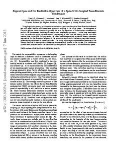
which we show in Figs. 1 and 2. The calculated chemical potential of a 3 × 3 array and a 9−site ring in the minimal Hubbard model approximation (Vii = U 6= 0, Vij = 0) is shown as a function of the applied flux φ in Fig. 1. Each curve in Fig. 1a (c) traces the chemical potential µN of a 3×3 array (L = 9 sites ring) with N electrons as a function of the magnetic flux φ/φ0 through a unit cell (the ring), with φ0 = h/e. The z-component (Sz ) of the total spin of the corresponding ground state of the system is shown in Fig. 1 (b) and (d), and the critical magnetic flux for full spin polarization in the array and the ring is given as an inset in Fig. 1 (a) and (c), respectively. The three main features of the results shown in Fig. 1 are: (a) the chemical potential spectrum evolves with the maximization of the total spin polarization in the system; (b) apart from an aperiodic single-particle background contribution, µ(N) is a periodic function of the magnetic flux with a flux periodicity of γ φ0 with γ ≤ 1; (c) the spin polarization transition of the system occurs through the cycles of the periodic Sz oscillations in the weak magnetic field region. The result (a) is a trivial outcome of the minimal Hubbard model: a dominant Zeeman energy term g ∗ µB leads to single-occupancy, effectively suppressing the presence of the Hubbard U term in Eq. 1. The chemical potential spectrum therefore behaves as that of noninteracting spinless fermions in the maximum spin-polarization region. The energy spectra of the 9−site systems plotted in Fig. 2(a) and in Fig. 7 for noninteracting quasiparticles [setting ε↓ = ∆, N = M in Eq. 1] can be directly compared with the strong field regions in Figs. 1(a) and (c). In the weak field region the single-particle physics can again be distinguished from the collective physics, and the spectrum in this regime is plotted in Figs. 2(b) and (c) for the array and the ring, respectively. In Figs. 2(b) and (c) we set ε↓ = ∆, ε↑ = ∆+δ, where δ/∆(= 0.03) ≪ 1, and M corresponds to the minimum eigenvalue of Eq. 1 for a given N. (We keep a small field-independent shift δ between opposite spin single-particle states for our later discussion of the Sz oscillations.) The parameters of the Hamiltonian that we use in Eqs. (1)-(5) determine the value of the critical magnetic flux φc needed to produce full spin polarization in the 3 × 3 array to be φc ≈ 8t2 a2 /(g ∗µB U) ≈ 52φ0 9

with a lattice constant of a = 280 nm. For illustrative purposes we rescaled the magnetic flux by 1/32 to show the full behavior of the spectrum on a single scale in Figs. 1(a) - (d). (This rescaling physically corresponds to rescaling the lattice constant to ≈ a/6.) IV. PERSISTENT CURRENT

We first clarify the physical meaning of the intricate magnetic field dependence of the energy spectrum shown in Figs. 1 and 2. It is well-known24 that gauge invariance along with the single-valuedness of the electron wavefunction allows for the existence of a ground state persistent current in normal metal rings threading an external magnetic flux. The intrinsic magnetic moment associated with this persistent current, which is proportional to the persistent current itself in 1D rings, is an oscillatory function of the external flux with a period equal to the elementary flux quantum φ0 . The existence of such an oscillatory persistent current in normal metal rings has been experimentally verified4 . In finite 2D continuous systems no magnetization is expected classically.25 It is argued that the magnetization due to electron orbits along the edge of the sample exactly cancels the magnetization arising from the bulk orbits. In a quantum-mechanical description, however, the contribution from the edge states is expected to be statistically insignificant25 , and the bulk contributions lead to the famous Landau diamagnetism in macroscopic 2D systems. In mesoscopic systems the phase coherence length Lφ is comparable to the linear system size L, and as was shown in several theoretical papers26,27 , the edge states in this situation can carry a persistent current creating a paramagnetic moment in the continuous 2D geometries (e.g., a 2D disk-shaped quantum dot) comparable in magnitude to the Landau diamagnetic term. The Aharonov-Bohm effect leads to a flux periodicity of the magnetization carried by the edge states effectively forming a 1D ring geometry in continuous 2D mesoscopic systems. We characterize the ground state magnetization of finite 2D quantum dot arrays without resorting to an artificial separation of bulk and edge states (which are not really meaningfully distinguishable in small structures) by considering the lattice model. The lattice spectrum 10

contains the “edge” states, the “bulk” states, and all other electron states given by the superposition of all topologically closed electron paths in the finite 2D lattice. The part of the Hamiltonian in Eq. 1 leading to the persistent current is the kinetic energy “hopping” (KE)hop term in Eq. 4. The total current operator28 is given by the commutator of the Hamiltonian with the polarization operator JT =

X ı Ri n ˆi. [H, P] , where P = −e h ¯ i

(7)

In a discrete lattice subjected to a magnetic field, the above formula becomes JT = −

n o 4π X (Rj − Ri) Im tij,α eıφij c† iα cjα . φ0 , α

(8)

The expectation value of the total current operator is zero in the ground state of an isolated finite quantum dot lattice. Then each divergenceless term in the sum of Eq. 8 can be identified as the current between two nearest neighbor lattice sites i and j: Jij = −

n o 4π X (Rj − Ri ) Im tij,α eiφij c† iα cjα . φ0 α

(9)

The magnetic moment operator is M=

1 2

Z

R × J(R) d3 R.

(10)

The magnetization density operator has a non-vanishing z-component (i.e. along the magnetic field direction) given by mz =

X Mz 1 Jij [xi (yj − yi ) − yi(xj − xi )] . = Area 2 ncells

(11)

Apart from the field dependence of single-particle levels in a single dot, the derivative of the Hamiltonian in Eq. 1 with respect to the flux is ∂H 2 ∂H = = ∂Φ ncells ∂φ ncells

X

, α

∂φij ∂φ

!

Im

n

o

tij,α eıφij c† iα cjα .

(12)

~ = (−B y , B x , 0) in a uniform field, and one gets for the AharonovIn a symmetric gauge, A 2 2 Bohm phase φij : 11

∂φij 2π xi yi = (yj − yi) − (xj − xi ) . ∂φ φ0 2 2 



(13)

The two operators in Eqs. 11 and 12 are equivalent, and therefore mz ≡ −

∂H . ncells ∂φ

(14)

Eq. 14 is the usual thermodynamic expression for the magnetization, which we have derived here for our microscopic model. In this paper we use the convention of calling the magnetization density mz the persistent current I in both 1D and 2D systems: I ≡ mz = −

∂H . ncells ∂φ

(15)

Experimentally, the equilibrium persistent current is usually observed by measuring the ground state magnetization.

V. THE NON-INTERACTING SPECTRA

We consider first the Hofstadter problem29 of a single particle in a magnetic field on an ~ = (0, Bx, 0), the discrete Schr¨ infinite tight-binding lattice. In the Landau gauge, A odinger equation in the occupation basis |αi = −i2π φφ x

ψ(x + 1, y) + ψ(x − 1, y) + e

0

X

ψ(x, y) is

(x,y) i2π φφ x

ψ(x, y + 1) + e

0

ψ(x, y − 1) = −E/t ψ(x, y), (16)

where φ is the flux through a unit cell, and the lattice constant a is taken as the unit length. At φ = 0, an infinite system described by Eq. 16 is translationally invariant. The coefficients of Eq. 16 involve only x. The y− motion separates out29 assuming that the y−part of the wavefunction preserves its φ = 0 plane wave form: ψ(x, y) = A(ky ) ψ(ky , x) eıky y . The function ψ(ky , x) is a solution of 12

(17)

!

φ ψ(x + 1) + ψ(x − 1) + 2 cos 2π x − ky ψ(x) = −E/t ψ(x). φ0

(18)

Eq. 18 is the well-known Harper equation, describing a particle in a one-dimensional quasiperiodic potential. An infinite tight-binding lattice in a nonzero flux is no longer invariant under lattice translations. It has, however, been shown that it is invariant under magnetic translations30 by qa, whenever the flux through a unit cell is a rational fraction φ =

p q

φ0 of

the fundamental flux quantum with p and q being any two integers. The Harper equation spectrum has q energy bands at the rational fractional values of flux φ =

p q

φ0 . The magnetic

translations by qa define a magnetic unit cell with the total flux φ = pφ0 through the magnetic unit cell. At incommensurate flux values (i.e. when φ/φ0 is not rational) the spectrum becomes a Cantor set.29 The Cantor set spectrum has an infinite number of energy bands that exhibit a self-similar multifractal behavior. The energy spectrum of Eq. 18 is always a continuous function of the magnetic flux,29 independent of whether φ/φ0 is rational or irrational. This enables one to make a direct connection between the lattice and the continuum spectra, for example, in identifying Landau bands in the lattice spectrum. The basic features of the spectrum29 of Eq. 18 (which we will refer to as the Hofstadter spectrum), which are also pertinent for a finite lattice, are: (a) it is periodic in φ0 , E(φ) = E(φ + nφ0 ); (b) it is an even function of flux, E(φ) = E(−φ); (c) both E(φ) and −E(φ) belong to the spectrum; (d) the spectrum is bounded, −4t ≤ E(φ) ≤ 4t. A quarter of the Hofstadter spectrum plotted for rational values of the flux is shown in Fig. 3 where we explicitly label the first two Landau bands. The Landau bands are formed in the continuum limit when the magnetic length far exceeds the lattice constant, i.e. l0 =

q

(1/2π)(φ0 /φ) ≫

1. In the tight-binding model, the effective mass is m ≈ h ¯ 2 /2t. The energy levels in a lattice for l0 ≫ 1 are approximately given by the continuous system Landau level expression, En = h ¯ ωc (n + 21 ) with h ¯ ωc = 4πt φ/φ031 . For example, the ratios of the slopes of the first three Landau bands in Fig. 3 obey 23.4 : 15.1 : 5.5 ≈ 5 : 3 : 1. The analytical solution of Eq. 18 for rational flux values were recently obtained using the Bethe ansatz method.32 The complete spectrum is extremely complex, but a general feature of the spectrum which can 13

be seen in Fig. 3 and to which we will later return in our study of the persistent current in finite systems, is the presence of energy bands separated by large gaps. √ √ A quarter of the spectrum for a finite L × L = 15 × 15 (L = 225) lattice is shown in Fig. 4. A qualitative similarity between the spectra plotted in Figures 3 and 4 was pointed out in the literature31 : the presence of similar energy bands in the spectrum, where the gaps between the bands are filled by the edge states which necessarily exist in finite systems. A finite spectrum was studied earlier in connection with the Quantum Hall effect and mesoscopic Aharonov-Bohm fluctuations.31 The emphasis of these earlier studies was on the part of the spectrum where both the Landau bands and the edge states can be clearly identified (the region from (d) to (e) in Fig. 4). Using Eqs. (4) and (9), we calculate the persistent current distributions in finite lattices for all eigenstates of Eq. 16. We follow Ref. 31 in the identification of different regions of the spectrum and illustrate each region with a sample current and a charge density distribution shown in Fig. 5. The lower-half band √ states in the weak field31 regime (l0 > L) labeled (a), (b) and (c) in Figures 4 and 5 can be considered to be extended bulk states because the paths of the persistent current carried by these states extend across the sample with finite weights both at the boundaries and in the bulk. The sign of the current carried by these states oscillates, but as φ → 0 it is determined by the degree of the degeneracy g of the spectrum at φ = 0. We identify the first three Landau bands in the spectrum labeled (d), (e), and (f) in Figures 4 and 5 (the traces of the 4th and 5th bands can also be seen in the plot). The ratios of the slopes of the first three bands are comparable to those of the infinite tight-binding lattice, 20.2 : 14.1 : 5.3. It is interesting to note that the radii of the “large weight” persistent current orbits in Fig. 5 approximately satisfy the semiclassical expression for the cyclotron radius of the nth Landau √ band, Rn = l0 2n + 1. The ratios of the radii of the persistent current orbits of the first √ √ three Landau bands in Fig. 5 obey 5 : 4 : 2 ≈ 5 : 3 : 1. Thus the continuous system result approximately holds for a finite lattice as well: each nth Landau orbit accommodates one more flux quantum than the (n − 1)st band orbit.

14

For larger flux φ ≥

φ0 , 2π

the Landau levels form a more complicated but less degenerate

pattern. We label the representative states (g), (h), and (i) for this region. The distribution of the persistent current carried by these states appears to consist of disconnected orbits, which can be found anywhere in the lattice. Intuitively, the existence of these disconnected persistent current orbits is consistent with our general expectation that smaller quantization orbits should not be strongly affected by the confining potential. The gaps of the infinite system in Fig. 3 are filled with edge states between the bulk Landau levels and the branched Landau levels in Fig. 4. The current distributions of the representative edge states labeled (j), (k), and (l) in Fig. 4 are shown in Fig. 5. These edge states have the largest weights concentrated near the boundaries in agreement with these states being called the “edge” states. The edge states in the regions between branched Landau levels (state (l) in Figures 4 and 5) seem to have a more complicated spatial distribution than the state labeled (j). The persistent current orbits of the state (l) are still extended across the lattice. The sign of the current carried by edge states of the type (j) is paramagnetic in accordance with the semiclassical argument given by Peierls25 . The flux and energy separation between these states correspond to one added flux quantum through the total area of the sample. This is the origin of the periodic Aharonov-Bohm oscillations superimposed on a regular pattern of de Haas-van Alphen oscillations in the magnetization and in the magnetoconductance discussed earlier by Sivan and Imry31 . The total persistent current I of a system of N noninteracting spinless particles for two values of N selected in Figures 4 and 5 is shown in Fig. 6. From the symmetries of the L = L1/2 × L1/2 lattice spectrum, it follows that I(−φ) = −I(φ), I(φ + nφ0 ) = I(φ), and I(N) = I(L − N). The total current is given by the sum of currents carried by all occupied single-particle states, and it can be quite different from the persistent current carried at the Fermi energy. For example, in Fig. 6(a), at flux φ = 0.25 φ0 , the state at the Fermi energy is a 2nd Landau level bulk state (denoted (e) in Figures 4 and 5) which carries a diamagnetic persistent current. But the total persistent current is positive at this value of flux in Fig.

15

6(a), corresponding to the positive contributions from each filled edge state. The change in the sign of the current from paramagnetic to diamagnetic in the region from φ ≈ 0.1 φ0 to φ ≈ 0.2 φ0 corresponds to merging all first 26 levels into the lowest Landau band. This merging of edge states into bulk states was discussed in Ref. 31. A similar change of the sign of the persistent current can be seen in Fig. 6(b) for the region of flux from φ ≈ 0.3 φ0 to φ ≈ 0.37 φ0 , where the Fermi Energy crosses from the branched Landau states through an edge state into the lower Landau level branched states. As mentioned above, an analytical solution for the eigenvalues of the Hofstadter problem (Eq. 18) at rational values of flux on an infinite tight-binding lattice has very recently been obtained using the Bethe ansatz technique.32 The fact that an infinite 2D problem (Eq. 16) can be reduced to an effectively 1D problem (Eq. 18) is instrumental in using the Bethe ansatz technique. In a finite 2D lattice with open boundary conditions, a general solution is formally written as ψ(x, y) = A(ky ) ψ(ky , x) expıky y +A(−ky ) ψ(−ky , x) exp−ıky y ,

(19)

where ψ(ky , x) and ψ(−ky , x) are the formal solutions of Eq. 18. The motion in the x and y spatial directions generally can not be separated in Eq. (19). The difficulty encountered in obtaining an analytic solution for the spectrum of a finite lattice stems from our inability to factor out a ψ(x) factor in Eq. 19 corresponding to the opposite ky momenta of an infinite lattice. The origin of this is the breaking of the time-reversal symmetry by the magnetic field. Eq. 18 is not invariant under the ky → −ky transformation. However, for the two limiting values of the magnetic flux φ = 0 and φ = 0.5 φ0 , the time-reversal symmetry is not broken, and the finite lattice problem can be analytically solved by reducing it to two effectively one-dimensional problems. The exact solution for these two limiting values of flux is given by ψ(x, y) = A(ky ) ψ(ky , x) sin(ky ), where ky takes on discrete values ky =

πn Ly +1

(20)

(n = 1, 2, ..., Ly ) with Ly being the extension 16

of the sample in the y−direction. The x part of the wavefunction in Eq. (20) satisfies the Harper equation, !

φ ψ(x + 1) + ψ(x − 1) + 2 cos 2π x cos(ky )ψ(x) = −E/t ψ(x). φ0

(21)

It can easily be verified by direct substitution that Eq. (20) is indeed a solution of Eq. (16) for the two limiting values of the flux, φ = 0 and φ = 0.5 φ0 . At φ = 0, Eqs. (20) and (21) reduce to a trivially diagonalizable problem with a solution given by the superposition of two independent standing waves in the x and y directions, ψ(kx ,ky ) = A(kx )A(ky ) sin(kx ) sin(ky ), and

(22)

E(kx ,ky ) = −2t(cos(kx ) + cos(ky )).

(23)

In Eqs. (22) and (23) the pseudomomenta kx and ky of a finite L = Lx × Ly lattice take the discrete values kx(y) =

πnx(y) , Lx(y) +1

with the integers nx(y) = 1, 2, ..., Lx(y) . The normalization

q

constants are A(kx(y) ) = 2/ 2Lx(y) + 1 [1 − sin[(2Lx(y) + 1)kx(y) ]/[(2Lx(y) + 1) sin kx(y) ]]−1/2 . We refer to the quantum numbers kx(y) as the pseudomomenta because the translational invariance is broken in a finite lattice, and the momentum is not a good quantum number. At φ = 0.5 φ0 , the problem reduces to solving the algebraic equation ∆m (E) = 0, where ∆m for m ≥ 2 obeys a recursion relation ∆m = [E/t − 2 cos(ky )]∆m−1 − ∆m−2 with ∆1 = (E/t)2 − 4 cos2 (ky ) and ∆0 = E/t − 2cos(ky ). We note that at φ = 0.5 φ0 , Eq. (21) has the symmetries of a bipartite lattice, and therefore the eigenspectrum is highly degenerate at this value of the flux. At φ = 0, we can characterize the spectrum using elementary group theory. A finite √ √ square L = L × L lattice has the symmetries of the C4v spatial point group. It is invariant under the following symmetry operations: (a) a rotation of the whole lattice by 2π; (b) a rotation by π; (c) a rotation by ±π/2; (d) a reflection around the vertical or horizontal axes of symmetry; and finally (e) a reflection about the two main diagonals of the lattice. These symmetry operations form 5 classes, and therefore the eigenstates of Eq. (16) 17

belong to 5 irreducible representations. The degeneracies are immediately deduced from the character table33 of the group C4v given in Table 1. The spectrum is either singly-degenerate, belonging to the one-dimensional A1, A2, B1, or B2 representation, or doubly-degenerate belonging to the two-dimensional E representation. In the last row of Table 1 we show the characters of the reducible representation of the group C4v of a 3×3 lattice in the occupation basis. Using the character table of the irreducible representations and the characters of this reducible representation, we deduce that for the 3×3 system, group theory predicts 2 pairs of doubly-degenerate eigenvalues and 5 singly-degenerate eigenvalues. Similarly, the number of √ √ degenerate states is deduced for a L × L lattice, and the results are given in Table 2. An √ √ √ additional electron-hole symmetry in the L × L problem mixes the L singly-degenerate states with total pseudomomenta kx + ky = π at zero energy. This can also be seen from Eq. √ √ (23). To summarize, for a finite square L × L lattice at φ = 0, we find g = 1 and g = 2 √ degenerate states in the spectrum as well as g = L degenerate states in the middle of the spectrum (see Figures 2(a) and 4 at φ = 0 for the examples of these spectra). As φ → 0 the magnetic field effects can be calculated in perturbation theory, where the perturbing Hamiltonian is given by the total persistent current operator y −1 Lx LX φ X x[c† (x,y+1) c(x,y) − h.c.]. H1 = −ıt2π φ0 x=1 y=1

(24)

At a small flux, the persistent current carried by the singly-degenerate states is linear in the flux in the lowest nonvanishing (2nd) order perturbation theory. The persistent current carried by the doubly-degenerate states is easily determined by a degenerate first order perturbation theory, where the 1st order correction to the energy is E 1 = ±|hγ|H1|βi with γ and β being the two doubly-degenerate states with the same energy at φ = 0. We summarize our results for the limiting values of flux for the 3 × 3 system in Table 3. For generic values of the flux, the spectrum of the 3 ×3 system is given by the solution of the eigenvalue problem of a 9 ×9 matrix. A symmetry operation which commutes with the finite two-dimensional square lattice Hamiltonian at φ 6= 0 will reduce the problem. In a particular gauge such a symmetry operation should leave invariant the Peirels phase factors in Eq. 18

~= (16). In both the symmetric (A

B (y, −x, 0)) 2

~ = B(0, x, 0)) gauge, upon and the Landau (A

transversing the distance between the two neighboring points (x1 , y1 ) and (x2 , y2 ) on a square lattice, the electron’s wavefunction gains a phase proportional to f (2, 1) = y2 x2 − x1 y1 . The object f (2, 1) is invariant under σv operations, which are reflections about the main diagonals of the lattice, i.e. x → y, y → x, and x → −y, y → −x. It is easy to verify that this symmetry is indeed observed in the numerically calculated current distributions in Fig. 5. In these gauges the σv operations exhaust all the spatial symmetries, but we can not rigorously prove that this result is gauge invariant. We can, however, comment on the degeneracies (or level crossings) which occur in the spectrum in Fig. 2(a) at φ =

1 8

nφ0 , n = 1, 2, 3, 4.

The limiting cases are given in Table 3. The degeneracy at φ = 0.25 φ0 at zero energy follows from the particle-hole symmetry. The values of flux at which the degeneracies occur, φ=

1 8

φ0 and φ =

3 8

φ0 , are the values when the first and second semiclassical orbits are

commensurate with the lattice. In a one-dimensional ring of length L enclosing a magnetic flux φ, the symmetry operator which commutes with the Hamiltonian is the magnetic translation operator along the ring, and the one-dimensional problem is easily diagonalized for all values of the flux with a spectrum given by14 "

2π En = −2t cos L

!#

φ +n φ0

,

(25)

where n = 1, ..., L. At a finite flux, the eigenstates of the ring Hamiltonian are also the eigenstates of the momentum, which are obtained from the momentum at φ = 0 by the same shift

2π φ ( ) L φ0

for all eigenstates. (As we shall show later, this result also holds in an

interacting one-dimensional Hubbard ring.) The energy level crossings between any two different n and n′ states occur at φ satisfying n − n′ = 2 φφ0 + 2 (integer). The resultant energy spectrum is periodic in φ (with a period φ0 ) through the ring. The discontinuities in the persistent current occur at φ = 0 (φ = 0.5) for even (odd) total number of electrons in the ring.14 A typical spectrum of a 1D tight-binding ring is shown in Fig. 7 for the L = 9 site ring. 19

It is of interest to compare the relative magnitudes of the 1D and 2D non-interacting persistent currents. In the 1D ring with N electrons the total current I(N, φ) is of the same order as the persistent current carried by the occupied individual states. This happens due to the cancelation of the persistent currents carried by the states with opposite momenta in the ground state distribution. In one period, I(N, φ) in the 1D ring is given by !

2π φ sin(πN/L) φ I(Nodd ) = −I0 sin , −0.5 ≤ ≤ 0.5, and L φ0 sin(π/L) φ0 ! ! # " φ φ 2π φ sin((N + 1)π/L) 2π N/2 + − sin , 0≤ ≤ 1, I(Neven ) = I0 sin L φ0 L φ0 sin(π/L) φ0

(26) (27)

where I0 = evF /L with vF = 2t/¯ h. Similar formulas were derived in Ref. 14. In a 2D system, the magnitude of the total current can decrease due to the cancelation between opposite sign persistent current contributions coming from bulk and edge states. In our earlier work,11 we showed that the typical 2D persistent current hI 2 i1/2 scales with the size of the boundary of the system. For completeness, we reproduce in Fig. 8 our results for the calculated systemsize dependence of the typical current in the half-filled 1D and 2D systems with the same flux through the areas of each system. In the case of a constant flux density (i.e., the same flux piercing a unit cell for different systems), the magnetization density (or the persistent current) saturates for large system sizes of 2D lattices for all electron fillings as shown in Fig. 9.

VI. THE INTERACTING SPECTRA

A. The minimal Hubbard model

1. Periodic Sz oscillations

A puzzling and interesting feature of the results plotted in Figs. 1 and 2 is the periodic oscillations of the z-component Sz of the total spin in the ground state of a finite quantum dot array. The existence of spin flips in the ground state by itself is not surprising. Any level crossing between states with different spins leads necessarily to a spin flip. The presence of 20

another flux value within a magnetic period that leads to a reverse flip can not be assumed a priori. This implies that the lowest energy states with different Sz can be degenerate for a range of the magnetic flux or at discrete flux values. We show in Fig. 10 the magnetic flux dependence of the ground state energy of the 3 × 3 array in the minimal Hubbard model (Eq. (5)) for values of N and M for which we find the Sz oscillations in Fig. 2(b). To obtain the results in Fig. 10, we set εi↑ = εi↓ = 0, and also leave out the terms not contributing to the Sz oscillations and consider an interaction of the local form Vint =

L X

U ρˆi↑ ρˆi↓ in Eq. (5).

i=1

The ground state energy with fixed N and M as a function of the flux appears to consist of segments of parabolas with their centers shifted along both the field and energy axes. For N = 2, 3, 4, 5, 6 in Fig. 10, the energy parabolas belonging to different M values overlap for a range of flux, leading to periodic Sz oscillations in Fig. 2(b) for a non-zero Zeeman splitting. This result is not restricted to 2D systems. We find it to be valid also in 1D rings. We show in Fig. 11 the flux dependence of the lowest energy with different N and M for which we find Sz oscillations in Fig. 2(c) in the Hubbard ring with L = 9 sites. In the rest of this subsection, we solve the Bethe ansatz equations to study the Sz degeneracy of the ground state of a 1D Hubbard ring and then generalize our results to two dimensions. The energy and the canonical momentum of an L-site Hubbard ring with N electrons enclosing a magnetic flux φ are given by the Bethe ansatz solution E = −2 P =

N X

j=1

"



#

N X

cos kj ,

(28)

j=1



X 2π X 2π φ Ij + = kj − Jα  . L φ0 L j α

(29)

(For the sake of brevity, we refer to the canonical momentum defined in Eq. (29) as the momentum from now on.) The energy and the momentum of the interacting system in Eqs. (28) and (29) are given by expressions similar to those for a non-interacting system, involving a summation over N pseudomomenta kj . The pseudomomenta kj describe the charge degrees of freedom that are coupled to the spin degrees of freedom with associated spin quantum numbers λα in an interacting system. The set of numbers kj and λα , referred 21

to as charge and spin rapidities, is found34 by solving a set of coupled Bethe ansatz equations: M X φ sin kj − λβ Lkj = 2πIj + 2π − , 2 tan−1 φ0 β=1 U/4t

#

"

N X

j=1

−1

2 tan

"

M X λα − λβ λα − sin kj = 2πJα + 2 tan−1 . U/4t U/2t β=1

"

#

#

(30) (31)

The quantum numbers Ij (Jα ) are integers if M is even (N-M is odd) and half-odd integers if M is odd (N-M is even), and Jα is restricted35 to a range |Jα | < (N − M + 1)/2. The ground state energy is obtained by taking the consecutive sets of integers Ij and Jα , and the lowest excitations are obtained by having holes in the ground state distribution of quantum numbers. The problem of the persistent current in a 1D Hubbard ring was studied earlier in Ref. 36. These authors found that the system accommodates magnetic flux by creating a magnon excitation with a hole in the ground state λα distribution. In Ref. 36 it was assumed that the spin excitations caused by the magnetic flux in the system remain spin waves for all values of U/t. This allowed one36 to conclude that for infinite U/t, the ground state energy has N cusps in a magnetic period. For large but finite U/t relevant to quantum dot arrays under investigation, the assumption that a magnetic field leads to a spin wave excitation in a 1D ring works well. In Appendix A, we reanalyze the ground state quantum number distribution of a Hubbard ring with particular values of N and M that were singled out in Ref. 36. In addition we analyze the ground state distributions of M − 1 states to understand the origin of the periodic Sz oscillations. To summarize our analysis of Appendix A, we find that a 1D Hubbard system of N interacting electrons behaves as a single particle on a ring in a magnetic flux: the ground state corresponds to a sequence of states with the consecutive values of the total momentum which are defined by Eq. (29). The resulting ground state energy has N intersecting parabolic segments per flux period for large U/t in agreement with Ref. 36. The interacting system changes its total momentum as a function of the flux by creating a magnon excitation. We find from the numerical solution of the Bethe ansatz Eqs. (28) - (31) that the dynamics 22

of this excitation (i.e. its location in the spectrum of spin rapidities) is determined by the dynamics of the total momentum that changes sequentially in multiples of 2π/L from its minimum to its maximum value within one magnetic period. This last finding was not emphasized in the earlier analysis36 of the persistent current in a Hubbard ring. This result follows from Eqs. (28) - (31) in the U/N → ∞ limit. In the limit of the infinite interaction, the pseudomomenta are given by 



2π X (L/2π)P φ kj = (1 − δjj ′ )Ij ′ + + . L j′ N φ0

(32)

A sequential set of the total momentum states which minimizes charge rapidities in Eq. (32) and, therefore, the ground state energy can be chosen by considering both, either spin or charge, excitations in the ground state quantum number distribution. The energy cost to create a charge excitation in the infinite interaction limit in a 1D Hubbard ring is associated with the motion of noninteracting spinless fermions and its magnitude is of the order of t. The energy cost to create a spin excitation is determined by t2 /U, leading to spin excitations being the most energy-efficient way in the 1D Hubbard ring to accommodate the enclosed magnetic flux. The total spin S may not change in a new total momentum ground state. Therefore, we find that all cusps in the ground state energy within a magnetic period are associated with changes in the orbital quantum numbers, but not necessarily with changes of the total spin. We find the ground states with nonzero total spin S to be the generic situation with respect to the magnitude of the interaction U/t, the electron filling, and the flux. Such ground states maintain their (2S + 1) degeneracy with respect to the different values of Sz over the range of the magnetic flux. This extended degeneracy is maintained until the total spin and momentum change in either of the different Sz ground states. In the presence of the extended total spin degeneracies a small nonzero Zeeman term (ωz ) in the Hamiltonian in Eq. (1) leads to the periodic oscillations of the z-component Sz of the total spin S as shown in Figs. 1 and 2. The reason is the following. For small ωz 6= 0 the ground state is the M = N/2 + 1 state, whereas for ωz = 0 the M = N/2 and M = N/2 + 1 states 23

are degenerate. Beyond this region, the M = N/2 state is the lowest energy state, and the system changes its Sz until it completes a period and the ground state again becomes M = N/2 + 1 state. In the 2D 3 × 3 array, similar extended total spin degeneracies with respect to the M, M − 1, M − 2 states lead to the Sz oscillations in Figs. 1 (a), (b) and 2(b).

2. Spin polarization transition

The critical magnetic field Bc characterizing the spin polarization transition in the min2

2

imal Hubbard model is determined to be gµB Bc ≈ 7.5 tU and ≈ 11 tU at half-filling in the L = 9 ring and the 3 × 3 array, respectively (see insets to Figure 1). In an infinite system, the critical field Bc corresponds to a field driven ferromagnetic transition and was calculated by several authors for a 1D Hubbard ring neglecting the orbital contribution37 . For large U/t (strong interaction) the critical magnetic field in the ring depends on the filling n = N/L through the relation gµB Bc =

8t2 n[1 U

limit, the critical field at half-filling is gµB Bc =

− sin(2πn)/(2πn)]. In the thermodynamic 8t2 . U

2

Qualitatively, the high value (≈ 11 tU )

of the critical field in the finite 2D system is not surprising, since we expect the quantum fluctuations to have a larger disordering effect in 2D systems, raising the critical field. More quantitatively, this result can be understood as follows. The critical field determines the gap for the triplet excitations in the ferromagnetic phase. At half-filling, the critical field is then determined by gµB Bc = E0 (N = L, M = N − 1) − E0 (N = L, M = N) with E0 being the lowest eigenvalue of Eq. (1) for particular values of N and M. The energy of the spin polarized state is trivial, E0 (N, M = N) = −NgµB Bc /2. In a strongly interacting M = N − 1 case, a spin down electron will ‘attract’ a spin up hole. The energetically favorable configuration on a lattice corresponds to a single site being occupied by the spin down electron and the spin up hole, and all the other sites being singly occupied by the ferromagnetically aligned spin up electrons. All the electrons contribute the trivial Zeeman term to the total energy, but the site with the spin down electron and its spin up neighbors also contribute 24

the exchange energy Eexch . The total energy of the M = N − 1 spin up and one spin down electrons is E0 (N = L, M = N − 1) = −(N − 1)gµB Bc /2 + gµB Bc /2 + Eexch. Therefore, the critical field is determined by the exchange energy, gµB Bc = Eexch . The exchange energy is given by Eexch =

4t2 U

f (d) with f (d) being the number of spin up neighbors of the spin down

electron. In a 1D ring f (d) = 2, and in large 2D systems on the average f (d) = 4 in the nearest neighbor tight-binding square lattice. Note that our numerical result for Bc in finite 1D rings (Bc ≈ 7.5t2 /U) is reasonably close to the thermodynamic result (Bc = 8t2 /U). 3. Metal-insulator transition and spin ordering

The charge stiffness, Dc , which characterizes [Dc = 0 (6= 0) characterizes the Mott insulator (metal)] the degree of localization in a Mott-Hubbard system is defined for a 1D ring of L sites to be38–41 Dc =

L ∂ 2 E0 (φ) . 2 ∂φ2

(33)

Note that, by definition, the charge stiffness is the negative flux derivative of the persistent current: Dc ∼

∂I . ∂φ

In Fig. 13 we compare the noninteracting and interacting persistent

currents calculated in the minimal Hubbard model for the 3 × 3 array. The interacting persistent current is suppressed by orders of magnitude at half-filling, n = N/(2L) = 0.5. This is a finite size manifestation of the Mott-Hubbard metal-insulator transition as n → 0.5 and U/t 6= 0. For small values of the flux the localization effects due to the magnetic field are small, and the magnetic response is not strongly affected by interaction at low filling in the metallic phase as can be seen in Figs. 13 (a)-(d). The additional discontinuities of the persistent current in Fig. 13 arise from the total spin S or from accidental degeneracies that occur with no Zeeman term in the Hamiltonian. In the insulating phase (N = 9 in Fig. 13) the persistent current is suppressed by orders of magnitude from its noninteracting value. Apparently, the ground state is described by one set of quantum numbers in a magnetic period, leading to the absence of discontinuities of the persistent current. The magnetic 25

response is paramagnetic at zero flux. We verify this suppression of the magnitude and oscillations as well as the paramagnetic nature of the persistent current at half-filling by doing calculations for 2 × 2, 3 × 2, 4 × 2 and 3 × 3 quantum dot arrays; these results are shown in Fig. 14. The rate of the suppression of the persistent current with the increased strength of the interaction U/t in the half-filled 3 × 3 array depends on the orbital magnetic flux. We compare this rate in the 3 × 3 array for the two values of the flux, φ/φ0 = 0.1 and φ/φ0 = 0.4 in Fig. 15. The magnetic field localization at φ/φ0 = 0.4 enhances the effect of the Hubbard U/t on the magnitude of the persistent current, compared to a slower decay of the persistent current at φ/φ0 = 0.1. Our use of the terms ‘insulating’ and ‘metallic’ to describe the N = L and N < L finite Hubbard systems is justified on the basis of the existing work38–42 . Using the linear response theory it can be shown that the charge stiffness at zero flux in a 1D ring is proportional to the zero- temperature DC conductivity of the system, with the real part of the conductivity given by39,40 σ(ω) = 2πDc (φ = 0)δ(ω) + σreg (ω).

(34)

The σreg (ω) term gives the weight of the finite frequency part of the conductivity spectrum, and the coefficient D = 2πDc = πe2 (n/m), called the Drude weight, gives the zero frequency weight of the conductivity spectrum. In infinite systems, an insulator is characterized by D = Dc = 0, and a metal has D > 038 . However, in finite systems in the insulating phase Dc is small but nonzero, and is expected to reduce exponentially with increasing system size. Stafford and Millis derived an explicit asymptotic form for the scaling function of the charge stiffness in a half-filled Hubbard L-site ring (with L even)39 , ˜ Dc (L, φ = 0)|L→∞ = (−1)L/2+1 L1/2 D(U/t) exp[−L/ξ(U/t)].

(35)

˜ In Eq. (35) D(U/t) is a U/t dependent number, and ξ(U/t) is the localization length, that at small U/t behaves as39 lim ξ =

U →0

2t + U/2π + ... . ∆(U, t) 26

(36)

In Eq. (36) ∆(U, t) is the Lieb-Wu Hubbard gap34 for the charge excitations in the system, that is determined by ∆c (U, t) = E0 (N + 1, M) + E0 (N − 1, M) − 2E0 (N, M). Stafford and Millis also showed39 that in a 1D Hubbard ring the equal time T = 0 Green’s function decays exponentially as G(x) ∼ exp(−|x|/ξ). Therefore, the decay of the persistent current and that of the single-particle Green’s function are shown to be connected in a 1D Hubbard ring. In the 2D Hubbard model at half-filling, where exact thermodynamic results are not available, recent numerical work using Monte-Carlo methods42 demonstrated that the singleparticle Green’s function scales as G(x) ∼ exp(−|x|/ξ2 ) with a correlation length ξ2 showing a critical behavior different from the 1D case. For our purpose the important point is that a 2D Hubbard system at half-filling is a Mott insulator, so following the exact 1D result of Stafford and Millis we make the ansatz that the charge stiffness in a 2D finite system also √ scales in the same way as the 2D Green’s function, Dc ∼ exp −l/ξ2 (U/t) with l ∼ L being the characteristic linear size of the system. This provides some rationale for our assertion that N = L results for the finite clusters in Figs. 14 and 15 correspond to the insulating phase. In the 3 × 3 array, the persistent current flows along the perimeter of the cluster for all N, but the sign of the persistent current in the system can be either diamagnetic or paramagnetic. Therefore, a steady paramagnetism that we find in the half-filled small arrays can not be understood using a simple analogy with the paramagnetism of the edge states in the corresponding noninteracting system25 . The sign of the noninteracting persistent current is paramagnetic in the half-filled 2 × 2, 4 × 2, and 3 × 3 arrays and is diamagnetic in the 3 × 2 array. The negative charge stiffness in the interacting 2 × 2 array is consistent with the prediction of Eq. (35) for a L = 4 × integer ring39,43 . We do not know whether this orbital paramagnetism is a generic feature of the finite half-filled 2D Hubbard lattices at zero temperature, but our finding is consistent with previous exact diagonalization studies of the optical conductivity of 4 × 4 periodic 2D Hubbard lattices which also found a negative Drude weight at half-filling44 . We have calculated the distribution of the local moments (h0|Sˆz,i|0i) in the half-filled finite lattices with the Zeeman term set equal to zero in the 27

Hamiltonian. The ground state of the 3 × 3 array belongs to a doublet with the total spin S =

1 2

and Sz = ± 21 . At U = 0, the uncompensated moment in the system is distributed

along the diagonals of the lattice. At finite U, the off diagonal dots gain opposite magnetic moments, and the system is antiferromagnetically ordered. We verified that the magnitudes of the neighboring moments show a tendency to equalize with increasing U/t. Therefore, a many-body state in the 3 × 3 array at half-filling represents a finite-size realization of the Mott-Heisenberg insulator41 (antiferromagnetic at a finite U/t) ground state in the system, with a Mott-Hubbard gap opening in the charge excitations (as manifested in the strong suppression of the persistent current in Figs. 13-15). The ground state for the even Llattices is a singlet (S = 0, Sz = 0), with all the local moments being very small. In the 1D L = 9-site ring (S = 21 , Sz = ± 21 ), we do not find any ordering of the local moments. We conclude that in small clean 2D systems the onsite interactions strongly suppress (possibly exponentially at N = L) the magnetic response as N → L, and for N < L the onsite interactions have a much weaker destructive effect.

B. The extended Hubbard model

We consider first onsite and nearest neighbor off-site interactions in Eq. (5). We set Vii = U, and Vij = V if (ij) are nearest neighbor dots (Vij = 0 otherwise). Eq. (1) then has the form of an extended Hubbard model45–47 . The Hubbard U by itself leads to a spin density wave (SDW) commensurate with the lattice periodicity at half-filling in a 2D lattice. This SDW state has uniform onsite charge density, hˆ ρi i = 1. It is easy to see from Eq. (1) that at half filling the off-site interaction V prefers double occupancy on the alternating sites, e.g. hˆ ρi

odd i

= 2, and hˆ ρi

even i

= 0. The

minimum energy configuration for a large nonzero V is the charge density wave (CDW) state commensurate with the lattice. The competition between U and V leads to a SDW-CDW transition in both 1D and 2D half-filled systems45–47 as V is increased. The mean field phase diagram is easily obtained by considering the strong coupling limits of U and V in Eq. (1). 28

The energy of the SDW state in the half-filled system is ESDW =

U N 2

+

V N 2 nn

with Nnn

being the number of all pairs of nearest neighbors on a lattice. The corresponding energy of the CDW state is ECDW = 4 U2 N2 . The phase transition line at half-filling in the extended Hubbard model is consequently given by V = Vc = U

N , Nnn

(37)

with V < Vc being the SDW state. In the 2D lattices with open boundary conditions, Nnn = 2L − Lx − Ly yields for large L, Vc ≈

U , 2

and in the 1D rings Nnn = L with

Vc = U. In the usual Hubbard model with periodic boundary conditions, the corresponding equations for the SDW-CDW phase transition are Vc =

U 4

(2D) and Vc =

U 2

(1D). In the half-

filled 1D finite rings the charge stiffness maximizes at the transition line between SDW and CDW states46 . Intuitively, this seems plausible because the persistent current is sensitive to quantum fluctuations, which are maximized at the phase transition. We find a similar maximization at half filling (N = 9) of the magnitude of the persistent current in the 3 × 3 2D array as a function of the off-site interaction V /t (Fig. 16). The persistent current is strongly suppressed on both sides of the SDW-CDW transition while being enhanced at the transition point. The current also changes sign at the transition and is more strongly suppressed deep in the CDW phase for large U/t. The critical interaction strength Vc = 0.65 at which the finite size SDW-CDW ‘transition’ occurs in the 2D array does not depend on the orbital magnetic flux (for U/t = 10), which is qualitatively consistent with the mean field and strong coupling results. The shape of the peak in Fig. 16, however, depends strongly on the orbital magnetic flux – the transition at a flux of φ/φ0 = 0.4 showing a larger enhancement than that at φ/φ0 = 0.1. The SDW-CDW transition in a 1D extended Hubbard model is found45 to be a second order phase transition for U/t < Uc /t = 3, and a first order transition for U/t > Uc /t. For example, the order parameter of the CDW state p = (1/N)

X i

(−1)i hˆ ρi i is nonzero in both

SDW and CDW phases for U > Uc 45,46 . A recent mean field calculation of the SDW-CDW phase diagram finds the transition to be first order (i.e. discontinuous in the order parameter) 29

for all values of U and V 47 . In the 3 ×3 system finite size effects dominate for weak coupling, < 3. We have and the persistent current peak position depends on the orbital flux for U/t ∼ calculated the persistent current as a function of V /t for U/t = 3, 5, 7, 10, 20, and 30 in the half filled 3 × 3 array and obtained the finite size SDW-CDW phase diagram, which is shown in Fig. 17. The slope of ≈ 0.68 of the linear fit to the data in Fig. 17 approximately agrees with the value 3/4 predicted within the strong coupling theory. With the inclusion of the longer range (beyond nearest neighbors) off-site interactions in our calculations, we find that the spin antiferromagnetic order is destroyed in the finite 3 × 3 array with the electron density distribution remaining uniform. We set the values of Vij using the classical capacitance matrix formalism7,8 as explained in Section II, and show in Fig. 18 our calculated persistent current at half filling (N = 9) as a function of V /t = (U/t)(C/Cg ), with U/t = (e2 /Cg )/t = 10 being fixed in the 3 × 3 array. An important conclusion from Fig. 18 is that strong long range interactions could enhance the magnitude of the persistent current back to its non-interacting half filled value, thereby effectively negating the Mott-Hubbard localization effect. Whether this is a general result (i.e. valid even in the thermodynamic limit) or purely a finite size effect is not clear at this stage. The intermediate values of the long-range interaction do not significantly modify the persistent current for N < L. This can be seen in Fig. 19 where we compare the (U/t = 10, V = 0) and (U/t = 10, V /t = 5) persistent current for various filling fractions in the 3 × 3 array. Our results can be understood on the basis of the dependence of the inverse capacitance matrix elements on the relative ratio of C/Cg . For simplicity, let us discuss this dependence in a double-dot array. In the limit C/Cg ≪ 1, the interdot and intradot interaction matrix elements are V12 = U(C/Cg ) → 0 and V11 = U. For C/Cg ≫ 1, these matrix elements are V12 = U/2 and V11 = (U/2)(1 + Cg /C) → U/2. The large ratio of C/Cg in the latter case effectively describes a single composite system. In this limit all elements of the inverse capacitance matrix become equal. Thus the electrons become totally uncorrelated, and the only effect of interactions is to give an overall charging energy to the system. Our results suggest that in a finite system with weakly screened interactions the SDW-CDW transition 30

may not occur, but the persistent current could still be enhanced to its noninteracting value.

VII. DISORDERED QUANTUM DOT ARRAYS

A. Non-interacting case

In this section we consider the effect of random disorder on the persistent current in the finite 2D quantum dot lattices in the spin polarized regime (see Figs. 2(a), 4 and 7 as examples of clean system spectra in this regime). We include disorder in our calculation through a spin-independent parameter W that denotes the half-width of a uniform distribution of random on-site quantum dot energies centered around ∆. The random on-site single-particle energies are set as εi = ∆ + δεi , δεi ǫ [−W/2, W/2].

(38)

The introduction of disorder could, in principle, lead to Anderson localization in the system, with all electronic states being exponentially localized in the presence of strong disorder20,48 . In general, disorder (W ) and interaction (U, V ) compete in determining the electronic properties of the resultant (W, U, V

6= 0) Mott-Hubbard-Anderson model.

Disorder introduces two related length scales in the problem: a mean free path l(W ) and a localization length ξ(W ). (In the absence of any interaction, in two dimensions for a weak disorder the localization length ξ(W ) depends exponentially20 on the mean free path as ξ = l exp[πkF l/2] with kF being the Fermi wavevector whereas in one dimension ξ ∼ l.) Scaling and perturbative arguments predict that for weak disorder (and in the absence of interaction) the conductance of a 2D lattice of size (L)2 depends logarithmically on the mean free path whereas for strong disorder it falls off exponentially with the system size as σ(L) ∼ exp(−L/ξ). We find two similar weak and strong disorder regimes in the behavior of the persistent current as a function of the disorder strength W , indicating a connection between the persistent current and the DC conductance of the finite 2D system. In one dimension Anderson localization occurs (i.e. σ(L) ∼ exp(−L/ξ)) in the presence of any 31

finite disorder20 , and the persistent current amplitude is exponentially suppressed14 for all W . In Fig. 20 we show the calculated log-log plot at half-filling of the rms current hI 2 i1/2 , averaged over 100 disorder realizations for each value of W , as a function of the disorder strength W for various array sizes (3 × 3, 4 × 4, 5 × 5, 6 × 6). In plotting these results, we have factored out a scale factor, nc /L = (L1/2 − 1)2 /L, so that the results for various system sizes fall on top of each other, showing approximate scaling with system size and disorder. (The scale factor nc = (L1/2 − 1)2 is the number of unit cells or plaquettes in each square array of size L.) The two dashed straight lines in Fig. 20 give the best fits to weak and strong disorder scaled currents, leading to the following empirical results for the effect of 1

disorder on the persistent current: hI 2 i 2

= (L/nc ) g(W ), with the scaling function g(W )

being given by g(W ) ∼

    W −γ ,

   W −β ,

γ = (6.4 ± 2.8) × 10−2, β = 1.84 ± 0.49,

W < 1.55 πt

(39)

W > 1.55 πt.

We note that the empirical scaling defined by Eq. 39 (and shown in Fig. 20) is consistent with well-known noninteracting scaling localization result of there being logarithmic 2D localization at weak disorder.

B. Interacting case

Random disorder effects on the persistent current are subtle in the presence of onsite interactions in the 3 × 3 array: they depend both on the filling in the array and the relative ratio U/W . Away from half-filling, the random disorder suppresses the magnitude of the current and smoothens its discontinuities arising from level crossings of energies with different orbital quantum numbers. The Sz oscillations and the corresponding discontinuities in < the current in the metallic phase persist in the presence of intermediate ( W ∼ U) disorder. Hubbard interaction effects are not particularly important at high disorder, which is what is seen in Fig. 20 (asterisks) for the typical interacting current even at half filling. The intermediate disorder (W < U) produces an antilocalization effect at half-filling by enhancing 32

the persistent current from its finite U-suppressed value as can be seen in Fig. 21 (a) and (b). We also observe that the disordered persistent current is enhanced in the presence of the long range interaction from its U-suppressed value as can be seen in Fig. 21(c). Finally we note that the presence of disorder does not reverse the roles of the weak and strong orbital flux: the relative behaviors of persistent current at φ/φ0 = 0.1 and φ/φ0 = 0.4 in Fig. 21 can be compared with those for clean systems plotted in Figs. 15 and 18.

VIII. CONCLUSIONS

We calculate the persistent current and electron addition spectrum in coherent twodimensional semiconductor quantum dot arrays and one-dimensional quantum dot rings pierced by an external magnetic flux, using the exact diagonalization and the Bethe ansatz techniques within an extended Mott-Hubbard Hamiltonian. We find that the magnetization density of a finite multidot array is periodic in the magnetic flux. In weak fields, we find flux periodic oscillations in the Sz component of the total spin S. We have included in our model the effects of both intradot/interdot Coulomb interactions and random disorder. We find that the persistent current is suppressed in the antiferromagnetic Mott-insulating phase. The finite-size realization of the spin density wave - charge density wave ordering transition has been found to maximize the 2D array persistent current at half-filling at the critical value of the nearest neighbor interaction, a behavior qualitatively similar to the charge stiffness of 1D rings46 . We obtain the phase diagram for the SDW-CDW transition. We demonstrate that the electrostatic long-range interdot interactions enhance the magnitude of the Mottinsulating phase persistent current to its non-interacting system value. We find that the noninteracting persistent current as a function of the random disorder strength exhibits a behavior similar to that of the conductivity20 of the system: it is strongly suppressed only at large disorder strengths. The Anderson-Mott transition48 has been found to have a subtle effect on the persistent current in the 3 × 3 array at half filling: the intradot Coulomb < interaction less than or comparable to the disorder strength W (U ∼ W ) increases the 33

disordered system persistent current. We believe that the 2D persistent current physics in the 3 × 3 array discussed in this paper has already been indirectly observed in transport measurements in a 3 × 3 array of strongly coupled quantum dots fabricated by means of square grid gate structures on top of a GaAs/AlGaAs heterostructure5 . In low magnetic fields (B < 1 T ) at T ≈ 40 mK the three conductance minima were measured in Ref. 5 at B=0.18 T, B=0.48 T, and B=0.80 T, and superimposed on these minima small oscillations periodic in B with period of 12 mT, 21 mT, and 24 mT were seen5 in the measured magnetoconductance of the 3 × 3 array. The large conductance minima were interpreted to be due to the classical localized orbits in the array, with the cyclotron radius of each orbit being equal to Rc = m∗ vF /eB, with Rc = 330 nm, 125 nm, and 75 nm in the three minima, respectively. The measured period of small oscillations was attributed to a reduction of a single classical orbit Aharonov-Bohm period due to the coupling between all possible classical orbits with a given Rc in the lattice. We suggest here an alternative explanation of this experiment. First, the observed large conductance minima correspond to the first three Landau orbits being commensurate with the size of a single dot. The semiclassical cyclotron radii, Rn =

q

(¯ h/eB)(2n + 1), are 60.5

nm (n=0), 64 nm (n=1), and 64 nm (n=2) for the three conductance minima, respectively. Therefore, we estimate the radius of each dot as 63 nm (which is reasonably consistent with the other dimensions of the array). These minima should be observed for temperatures for which h ¯ ωc ≤ 2kT yielding T ≈ 1.8 K, which is consistent with T = 2 K where the large conductance minima start to be affected by the temperature5 . We agree with the experimentalists that the shorter period oscillations are due to the coupling of the electron orbits in the lattice. But we think that the contributing orbits originate from the quantum mechanically required gauge invariance in the experimental phase coherent system. These orbits arise due to electron hopping between the localized states of each dot. We estimate that the magnetic flux corresponding to one flux quantum φ0 piercing a unit cell of the lattice is ≈ 46 mT (with a lattice constant of a ≈ 300 nm). For the density of the 2DEG and the estimated size of the dot, the number of electrons in each dot is ≈ 5. Considering one 34

mobile electron at the Fermi energy in each dot, the experimental 3 × 3 array approximately corresponds to our 3 × 3 array at half filling (in the situation of the weakly screened longrange Coulomb interactions). The persistent current in our case is found to oscillate with a period of φ/φ0 = 0.25 and 0.5 (see Figs. 13(h) and 19(h)), that corresponds to ∆B = 11.5 mT and ∆B = 23 mT, which are consistent with the experimentally measured values. Finally, we emphasize three essential limitations of our work which may (generally) restrict its quantitative applicability to realistic quantum dot arrays (we do believe that our results describe well the qualitative aspects of coherent and collective physics in semiconductor quantum dot arrays): (1) we ignore completely the complicated (and interesting) details of single dot electronic structure, approximating the energy level in each dot by two spin-split energy levels described by the simple Fock-Darwin-Zeeman model; (2) we use the Mott-Hubbard model in treating interaction and correlation effects (both intradot and interdot) – such a simple parameterization of Coulomb correlations may not apply quantitatively in real quantum dot arrays; (3) we have considered only small (no more than 9 dots) finite arrays, being limited entirely by the exponentially growing Hilbert space size in our extended Hubbard model. While we see no particular hope of going beyond these approximations in the near future, we should emphasize that these limitations do not substantially restrict the qualitative applicability of our results to the coherent collective physics of quantum dot arrays. For example, currently fabricated coherent quantum dot arrays typically contain only two to four quantum dots, and therefore our finite size calculations are, in fact, perfectly appropriate. Also, the basic physics of Coulomb blockade and quantum fluctuations are entirely captured in our extended Mott-Hubbard model, and the complications of single dot energetics (beyond that of two-level Fock-Darwin-Zeeman physics) can usually be distinguished from the collective physics of interest to us. Finally, some of our non-essential approximations, for example, restricting to zero temperature and using a constant interdot hopping amplitude t, can easily be relaxed in future calculations if such a need arises. We emphasize here that these non-essential approximations do not affect our qualitative conclusions in any significant manner. We believe that the extended finite Mott-Hubbard model as 35

used by us is the appropriate minimal model which should form the basis of discussing the collective and coherent physics in mesoscopic semiconductor quantum dot arrays. We feel that the direct observation of equilibrium persistent current and spin oscillations in coherent quantum dot square lattices and rings will shed light on the interplay among the single dot physics, coherence, disorder, long- and short-range Coulomb interaction effects on quantum phase transitions that we discuss in this paper. This work was supported by the U.S.-O.N.R.

APPENDIX A: GROUND STATE ENERGY OF A HUBBARD RING ENCLOSING A MAGNETIC FLUX

Here we analyze the ground state quantum number distribution of a Hubbard ring that we obtain by solving numerically the Bethe ansatz Eqs. (28) - (31) for all N < L, M = N/2 and M = N/2 − 1. a. N = 4n + 2, M = 2n + 1, and M = 2n. For N = 4n + 2 and M = 2n + 1 the ground state distribution at a flux φ ≥ 0 is given by36 : (N − 1) (N − 1) (N − 1) ,− + 1, ..., , and (A1) 2 2 2 (M − 1) (M − 1) (M − 1) (M − 1) (M − 1) − 1, − , ..., − + p − 1, − + p + 1, ..., . (A2) {Jα } = − 2 2 2 2 2 {Ij } = −

In Eq. (A2) the position p of a hole in the distribution of the spin rapidities varies from p = 0 to p = M within one half of a magnetic period, and p = 0 corresponds to the ground state distribution at φ = 0. The ground state distribution for negative values of the flux is obtained by shifting all Jα to the right by one unit. The momentum P of the state is given by the momentum q of the spin wave excitation P = q = − 2π p. Thus, the total momentum is zero L within one half of at zero flux and then takes the values of all consecutive multiples of − 2π L magnetic period, with the momentum being equal to

L P 2π

= −M = − N2 at φ/φ0 = 0.5. The

distribution in Eq. (A2) is valid for N < L, for N = L the distribution of both the charge and spin quantum numbers remains symmetric at a nonzero flux. Since 36

L P 2π max

= − N2 , in

1 the limit of large U/t the ground state energy has N cusps at φ/φ0 = ±(p + 1) 2N , and the 1 . It was proved by Stafford and Millis39 persistent current is diamagnetic at φ/φ0 = ±p 2N

that the N = 4n + 2 ground state of the electron system under periodic boundary conditions is a spin singlet (total spin S = 0) at φ = 0, and it can be either a spin triplet (total spin S = 1) or a singlet at φ = 0.5 φ0 (a flux value where the antiperiodic boundary conditions are realized). In the L = 9-site Hubbard ring we find that at φ = 0, the ground state is a spin singlet, and at φ = 0.5 φ0 it is a spin triplet with S = 1. At φ = 0.5 φ0 , the ground state, therefore, has a (2S + 1) spin degeneracy. The energy of the N = 4n + 2 and M = 2n (Sz = 1) state is higher than the ground state energy of the singlet state at φ = 0 (as an example, see Fig. 11(d) for N = 6, M = 3, and M = 2). The energy of the Sz = 1 state at φ ≥ 0 is minimized by choosing the ground state distribution as N N N , − + 1, ..., − 1, and 2 2 2 (M − 1) (M − 1) (M − 1) (M − 1) , ..., − p, − − p + 2, ..., + 1. {Jα } = − 2 2 2 2 {Ij } = −

(A3) (A4)

In Eq. (A4) the position p of a hole in the distribution of the spin rapidities varies from p = M to p = 0 within one half of a magnetic period, and p = M corresponds to a ground state distribution at φ = 0. The charge degrees of freedom contain a nonzero momentum

L r 2π

= − N2 in the system, and the spin rapidities are positioned in the Fermi sea

to minimize the total momentum at φ = 0. The vacant hole in this system is also within the Fermi bounds. The total momentum of the state described by Eqs. (A3) and (A4) is L P 2π

are

= −( N2 − p). Thus, at φ = 0 and φ/φ0 = 0.5, the minimum and maximum momenta L P 2π

= −1 and

L P 2π

= − N2 , respectively. Within our numerical accuracy we do not

find that the excitation can create a zero total momentum at φ = 0 in the range of the interaction U/t values from 0 to 200. Therefore, at φ = 0, there is a cusp corresponding to the crossing of equal and opposite minimum momenta, and the ground state energy has a total of N − 1 cusps per magnetic period. The spin quantum numbers of the N = L ground state remain symmetric in a magnetic period. The Sz = 0 and the Sz = 1 states have the 37

same total momenta at the last segments of the energy curves that includes φ = 0.5 φ0 . This is a situation for the N = 6, M = 3 and N = 6, M = 2 states in the L = 9-site ring at φ = 0.5 φ0 in Fig. 11(d). The total spin of the M = 2 system does not change in a magnetic period and is equal to 1. The degenerate M = 3 and M = 2 states belong to a spin triplet in the segment of the energy curve centered at φ = 0.5 φ0 . We conclude that the magnetic flux changes the total momentum of a state sequentially by one unit from one parabola segment to another (for smaller values of U/t, particular values of the total momenta are missing in the ground state36 ). Each energy parabola segment has a fixed value of the total spin, which may or may not change with a change of the total momenta. The extended degenerate nonzero total spin regions are not specific to the ground state of the N = 4n + 2 systems. They occur whenever the magnetic field drives the systems with different Sz through a series of the consecutive total momentum states to the flux region where the ground state has a nonzero total spin S and the different Sz states thus have the same total momenta. b. N = 4n, M = 2n, and M = 2n − 1. For N = 4n (N < L) and M = 2n the ground state distribution at a flux φ ≥ 0 is the same as for N = 4n + 2 and M = 2n case that is given in Eqs. (A3) and (A4). In the current situation, a spin wave excitation is above the Fermi sea, and the minimum momentum is

L P 2π

= −( N2 − M) = 0 at φ = 0. The ground

state energy has N cusps in a period,36 and the persistent current is diamagnetic at the 1 φ/φ0 = ±p 2N . The ground state distribution for N = 4n and M = 2n − 1 is given in Eqs.

(A1) and (A2). For large U/t, an excitation above the negative Fermi sea of spin rapidities can be created, so the momentum at φ/φ0 = 0.5 is

L P 2π

= − N2 . The Sz = 0 and Sz = 1

states can have the same minimum momenta P = 0 at φ = 0. In Fig. 11(c) for N = 4 electrons in the ring, the energy parabolas of M = 2 and M = 1 belonging to the spin triplet (S = 1) states are coincident in the P = 0 magnetic flux region centered at φ = 0. For N = 8 in Fig. 11(e) the levels of the P = 0 momentum triplet state (S = 1, Sz = 1) and

L P 2π

= ±4 singlet state (S = 0, Sz = 0) cross in the vicinity of φ = 0 and are non

degenerate at φ = 0. 38

c. N = 4n + 1, M = 2n, and M = 2n − 1. For N = 4n + 1 (N < L) and M = 2n electrons in a Hubbard ring, both sets of Ij and Jα are integer numbers. To accommodate the variation of the total momenta, two holes are present in the ground state distribution at a nonzero positive flux: (N − 1) (N − 1) (N − 1) ,− + 1, ..., , and 2 2 2 M M M (M − 2) , ..., − + p2 − 2, − + p2 , ..., 0, ..., p1 − 1, p1 + 1, ..., . {Jα } = − 2 2 2 2 {Ij } = −

(A5) (A6)

In Eq. (A6) the position p1 of a hole in a distribution of spin rapidities varies from p1 = 0 at φ = 0 to p1 = from 0 to

M , 2

M 2

with p2 being fixed at p2 = 0. While the hole p1 transverses

the momentum varies from 0 to − M2 . A further increase of the momentum

is accomplished through the motion of the second hole p2 from 0 to fixed at

M . 2

M 2

− 1 with p1 being

The total momentum becomes P = − 2π M at φ/φ0 = 0.5. Therefore, in the L

ground state distribution there is always one hole which moves. We show the energies for consecutive values of the total momentum in a L = 15 ring for n = 2 and L = 9 ring for n = 1 for U/t = 200 in Fig. 12 (a) and (b), respectively. The ground state energy curves in Fig. 12 (a) and (b) consist of the N consecutive momentum states within a magnetic period. The earlier analysis of the persistent current in a Hubbard ring did not emphasize the dynamics of the total momentum, and Yu and Fowler mistakenly concluded that their Eq. (3.13) describes the ground state distribution for any nonzero flux, and that at the one half flux quantum all the Jα ’s have to be consecutive integers36 . The charge and spin quantum numbers are half-odd integers for N = 4n + 1 and M = 2n − 1 electrons in a ring. The ground state distribution at φ ≥ 0 for n > 1 is given by N N N , − + 1, ..., − 1, and (A7) 2 2 2 M M 1 3 1 M M + 1. (A8) {Jα } = − , ..., − + p2 − 1, − + p2 + 1, ..., − , ..., − + p1 , + p1 , ..., 2 2 2 2 2 2 2 {Ij } = −

In Eq. (A8) the hole p1 moves from 0 to (M + 3)/2 with p2 being fixed at p2 = 0, and then the hole p2 moves from 0 to (M − 3)/2 while p1 = (M + 3)/2. The motion of the holes in the distribution of the spin rapidities leads to a cancelation of the −N/2 momentum 39

concentrated in the charge degrees of freedom at zero flux and the consequent integral decrease of the total momentum. In the L = 9 ring with N = 5 electrons, for the value of the interaction U/t = 10, the states M = 2 and M = 1 have different values of the total spin S =

1 2

and S =

3 2

and the total momenta

L P 2π

= −1 and

L P 2π

= −2, respectively. These

states are nondegenerate, and there are no oscillations of the total spin Sz in the ground state of the L = 9, N = 5 Hubbard ring. d. N = 4n − 1, M = 2n − 1, and M = 2n − 2. The lowest energy state for N = 4n − 1, M = 2n−1 is obtained by choosing the distribution of quantum numbers that is given in Eqs. (A7)-(A8). At zero flux, the hole p1 starts moving from Jα = 21 , and it moves (M + 1)/2 − 1 consecutive steps to the right. In the remaining flux region the hole p2 transverses to the right in (M − 1)/2 − 1 consecutive steps. The distribution in the M = 2n − 2 case is given in Eqs. (A5)-(A6). In this case the hole p2 moves until the total momentum becomes −(N + 1)/2 at φ/φ0 = 0.5. At φ = 0 for N = 3 electrons in a L = 9-sites ring in Fig. 11(b), the two lowest M = 1 and M = 0 energy states with momentum P = 0 and the total spin S=

3 2

are degenerate in the φ = 0 region.

40

REFERENCES 1

L. P. Kouwenhoven et al., Phys. Rev. Lett. 65, 361 (1990); D. Dixon et al., Phys. Rev. B 53, 12625 (1996); R. H. Blick et al., Phys. Rev. B 53, 7899 (1996); F. R. Waugh et al., Phys. Rev. Lett. 75, 705 (1995); F. R. Waugh et al., Phys. Rev. B 53, 1413 (1996); C.H. Crouch et al., Surface Science 361/362, 631 (1996); C. H. Crouch, PhD thesis (Harvard University, 1996); C. Livermore et al., Superlattices and microstructures 20, 633 (1996); O. Klein et al, Phys. Rev. Lett. 74, 785 (1995); N. C. van der Vaart et al., Phys. Rev. Lett. 74, 4702 (1995); F. Hofmann et al., Phys. Rev. B 51, 13872 (1995); A. Yacoby, M. Heiblum, D. Mahalu, and H. Shtrikman, Phys. Rev. Lett. 74, 4047 (1995).

2

C. Livermore, C. H. Crouch, private communication (1997).

3

R.C. Ashoori et al, Phys. Rev. Lett. 68, 3088 (1992); ibid., 71, 613 (1993).

4

L. P. Levy et al., Phys. Rev. Lett 64, 2074 (1990); V. Chandrasekhar, R. A. Webb et al., ibid 67, 3578 (1991); D. Mailly et al., ibid bf 70, 2020 (1993); B. Reulet et al., ibid 75, 127 (1995).

5

K.-M. H. Lenssen, M. E. J. Boonman, C. J. P. Harmans, C. T. Foxon, Phys. Rev. Lett. 74, 454 (1995).

6

G. Kirczenow, Phys. Rev. B 46, 1439 (1992).

7

P. Delsing, J. E. Mooij and G. Shon in Single Charge Tunneling, edited by H. Grabert and M. Devoret (Plenum, New York, 1992).

8

A. A. Middleton and N. S. Wingreen, Phys. Rev. Lett. 71, 3198 (1993).

9

C. A. Stafford and S. Das Sarma, Phys. Rev. Lett 72, 3590 (1994); C. A. Stafford and S. Das Sarma, Phys. Lett. A 230, 73 (1997).

10

G. Klimeck, G. Chen, and S. Datta, Phys. Rev. B 50, 2316 (1994); G. Klimeck, G. Chen, S. Datta, G. Chen, and W. A. Goddard III, Phys. Rev. B 50, 8035 (1994). 41

11

R. Kotlyar and S. Das Sarma, Phys. Rev. B 55, R10 205 (1997).

12

V. Fock, Z. Phys.47, 446 (1928).

13

Y. Imry, in Directions in Condensed Matter Physics, edited by G. Grinstein and G. Mazenko (World Scientific, Singapore, 1986), p. 101; S. Washburn and R. A. Webb, Adv. Phys. 35, 375 (1986).

14

Ho-Fai Cheung, E. K. Riedel, Y. Gefen, Phys. Rev. Lett. 62, 587 (1989); Ho -Fai Cheung et al., Phys. Rev. B 37, 6050 (1988).

15

B. S. Shastry and Bill Sutherland, Phys. Rev. Lett. 65, 243 (1990).

16

V. Ambegaokar and U. Eckern, Phys. Rev. Lett. 65, 381 (1990); A. M¨ uller-Groeling and H. A. Weidenm¨ uller, Phys. Rev. B 49, 4752 (1994); T. Giamarchi and B. S. Shastry, Phys. Rev. B 51, 10915 (1995); M. Kamal, Z. H. Musslimani and Assa Auerbach, J. Phys. I France 5, 1487 (1995); M. Ramin, B. Reulet, and Helene Bouchiat , Phys. Rev. B 51, 5582 (1995).

17

M. Abraham and R. Berkovits, Phys. Rev. Lett. 70, 1509 (1993); G. Bouzerar, D. Poilblanc, and D. Montambaux, Phys. Rev. B 49, 8258 (1994) ; T. Chakraborty, P. Pietil¨ ainen, Phys. Rev. B 52, 1932 (1995); W. Deng et al., Phys. Rev. B 50, 7655 (1994).

18

M. B¨ uttiker and C. A. Stafford, Phys. Rev. Lett., 495 (1996).

19

T. Chakraborty, P. Pietil¨ ainen, Phys. Rev. B 50, 1994 (1994); G. S. Jeon and M. Y. Choi, J. Phys.: Condensed Matter 8, 4429 (1996); G. Bouzerar and D. Poilblanc, Journal de physique. I 7, 877 (1997); C. A. Stafford and D. F. Wang, Phys. Rev. B 56, R4383 (1997); Z. Phys. B 103, 323 (1997).

20

P. A. Lee and T. V. Ramakrishnan, Rev. Mod. Phys. 57, 287 (1985).

21

A. Kumar et al., Phys. Rev. B 42, 5166 (1990).

22

R.E. Peierls, Z. Phys. 80, 763 (1933). 42

23

Jane K. Cullum, Ralph A. Willoughby in Lanczos Algorithms for Large Symmetric Eigenvalue Computations, Birkh¨auser Boston, Inc.: (1985).

24

F. London, J. Phys. Radium 8, 347 (1937); N. Byers and C. N. Yang, Phys. Rev. Lett 7,46 (1961); F. Bloch, Phys. Rev. 137, A 787 (1965); M. Buttiker, Y. Imry and R. Landauer, Phys. Lett. 96A, 365 (1983).

25

R. Peierls, Surprises in Theoretical Physics (Princeton University Press, Princeton, 1979), pp. 99-110.

26

B. L. Altshuler, Y. Gefen, and Y. Imry, Phys. Rev. Lett 66, 88 (1991).

27

C. W. J. Beenakker, H. van Houten, and A. A. M. Staring, Phys. Rev. B 44, 1657 (1991).

28

G. D. Mahan, Many-Particle Physics, 2-nd edition, Plenum Press, New York and London (1990).

29

Douglas R. Hofstadter, Phys. Rev. B. 14, 2239 (1976).

30

J. Zak, Phys. Rev 134, A1602-A1611 (1964).

31

U. Sivan and Y. Imry, Phys. Rev. Lett 61, 1001 (1988); U. Sivan, Y. Imry, and C. Hartzstein, Phys. Rev. B 39, 1242 (1989).

32

P. B. Wiegmann and A. V. Zabrodin, Phys. Rev. Lett. 72, 1890 (1994); P. B. Wiegmann and A. V. Zabrodin, NATO advanced study institutes series. Series B, Physics. 328, 399 (1995); L. D. Fadeev and R. M. Kashaev, Communications in mathematical physics 169, 181 (1995).

33

J. W. Leech and D. J. Newman in How to use Groups (Methuen and Co LTD and Science Paperbacks, London, 1969), pp. 29-34.

34

E. H. Lieb and F. Y. Wu, Phys. Rev. Lett. 20, 1445 (1968).

35

H. J. Schulz, in Correlated electron systems edited by V.J. Emery, World Scientific, Sin-

43

gapore, River Edge, NJ, (1993). 36

N. Yu and M. Fowler, Phys. Rev. B 45, 11795 (1992).

37

J. Carmelo, P. Horsch, P. A. Bares and A. A. Ovchinikov, Phys. Rev. B 44, 9967 (1991); Holger Frahm and V. E. Koperin, ibid. 43, (1991).

38

W. Kohn, Phys. Rev. 133, A171 (1964).

39

P. Maldague, Phys. Rev. B 16, 2437 (1977); C. A. Stafford and A. J. Millis, Phys. Rev. B 48, 1409 (1993).

40

D. J. Scalapino, S. R. White, S. Zhang, Phys. Rev. B 47, 7995 (1993).

41

F. Gebhard, The Mott Metal-Insulator Transition, Springer Tracts in Moder n Physics 137, Springer-Verlag Berlin Heidelberg New York (1997).

42

F. F. Assaad and M. Imada, Phys. Rev. Lett. 76, 3176 (1996).

43

C. A. Stafford, A. J. Millis, and B. S. Shastry, Phys. Rev. B 43, 13660 (1991).

44

E. Dagotto, A. Moreo, F. Ortolani, D. Poilblanc, and J. Riera, Phys. Rev. B 45, 10 741 (1992); E. Dagotto, Rev. Mod. Phys. 66, 763 (1994).

45

J. E. Hirsch, Phys. Rev. Lett. 53, 2327 (1984).

46

Q. Wang, Z. D. Wang and J.-X. Zhu, Phys. Rev. B 54, 8101 (1996).

47

B. Chattopadhyay and D. M. Gaitonde, cond-mat/9703213.

48

D. Belitz and T. Kirkpatrick, Rev. Mod. Phys. 66, 261 (1994), and references therein.

44

FIGURES FIG. 1. (a) [(c)] A chemical potential µN as a function of flux φ in units of φ0 = h/e through an elementary cell [a ring in (c)] of a 3 × 3 quantum dot lattice [9−site ring in (c)] with N (= 1 − 9) excess quasiparticles in the minimal Hubbard model approximation; (b) [(d)] A corresponding z-component Sz of the ground state total spin as a function of φ. The magnetic flux is rescaled by 1/32 to show the entire dynamics of the spectrum on one flux scale as explained in the text. Insets: The critical magnetic flux φc of the spin polarization transition as a function of the electron filling n = N/(2L) in the arrays. FIG. 2.

(a) A chemical potential spectrum plotted versus flux through a unit cell of a

non-interacting 3 × 3 array with ε↓ = ∆, N = M in Eq. (1); (b) [(c)] A chemical potential as a function of flux (top panel), and the corresponding Sz component of the ground state total spin (bottom panel) of a 3×3 array [9−site ring in (c)] with ε↓ = ∆, ε↑ = ∆(1+δ/∆) (δ/∆ = 0.03) in Eq. (1). (a), (b) and (c) can be directly compared with high and low field regimes in Figs. 1(a) and (c), respectively. FIG. 3. A spectrum of Eq. (16) plotted for rational fractions of flux φ/φ0 = p/q (q = 120, p is incremented from 1 to 60) through a unit cell of an infinite tight-binding lattice. The first two Landau bands (n = 0, 1) are marked on the plot. FIG. 4.

A spectrum of a finite 15 × 15 tight-binding lattice versus φ/φ0 through a unit cell.

The different regions that are marked (a)-(l) on the plot are discussed in the text. FIG. 5. The persistent current and charge density distribution of the single-particle states marked in Fig. 4. The darkness of circles, and darkness, or thickness of connecting lines are proportional to the magnitude of charge and current, respectively. Arrows on the lines show a direction of the persistent current. The maximum current and charge in (a) to (l) in units of (et/h) and e, respectively, are 0.028, 0.009; 0.114, 0.018; 0.232, 0.023; 0.250, 0.102; 0.393, 0.039; 0.150, 0.030; 0.162, 0.062; 0.172, 0.019; 0.126, 0.011; 0.161, 0.027; 0.073, 0.015; 0.099, 0.017.

45

FIG. 6. The total persistent current I calculated using Eq. (15) for (a) N = 26 electrons on a 15 × 15 lattice((e) in Figs. 4 and 5), and (b) N = 73 ((h) in Figs. 4 and 5). FIG. 7. The energy spectrum of a 9-site tight-binding ring shown for one period of flux through the area of a ring; this spectrum can be compared with the high field regime in Fig. 1(c). FIG. 8. hI 2 i1/2 at half filling versus system sizes (L) (L = L1/2 × L1/2 with L1/2 varying from 2 to 10): triangles (2D array), squares (1D ring). (The average is taken over the range of the same total flux through the systems, which varies from −φ0 /2 to φ0 /2.) The dashed lines are the best linear fits to the dependence hI 2 i1/2 ∼ Lα with α = 0.46 (1.1) in a 2D (1D) systems. FIG. 9. A typical current hI 2 i1/2 , I at φ = 0.25 φ0 , and the maximum current Imax are shown from top to bottom, respectively, as a function of N electrons in L1/2 × L1/2 systems (with L1/2 varying from 2 to 10) with the same flux density for systems of different sizes. FIG. 10. The energy of the 3 × 3 quantum dot array calculated using Eq. (1) in a minimal Hubbard model approximation ( V2ii = U = 10t, Vij = 0, ε↑ = ε↓ = 0) as a function of the flux through the unit cell. The energy is plotted for all values of N and M which are found in the ground state of the array in Fig. 2(b). In (a)-(f), a number of electrons N in the array is as indicated in the legend; M = N/2, M = N/2 − 1, M = N/2 − 2 energy states are shown with the solid, dotted, and dashed lines, respectively. The states with different M that are degenerate over the range of flux have the total spin in (a) S = 1; (b) S = 23 ; (c) S = 2, 1, 0; (d) S = 32 ; (e) S = 1.

46

FIG. 11. The energy of an 9−site Hubbard ring as a function of the flux through the ring calculated using the Bethe ansatz Eqs. (28)-(31). All parameters and plotting conventions are as given in the caption in Fig. 10. A sequence of states in one magnetic period, for the flux −0.5 ≤ φ/φ0 ≤ 0.5 is given by (a) L 2π P

= 1, 0, −1 (M = 1) and

(M = 1); (d) and

L 2π P

L 2π P

L 2π P

L 2π P

= 1, 0, −1 (M = 1) and

= 0 (M = 0); (c)

= 3, 0, −3 (M = 3), and

L 2π P

L 2π P

L 2π P

= 1, −1 (M = 0); (b)

= 2, 0, −2 (M = 2) and

= 3, 1, −1, −3 (M = 2); (e)

L 2π P

L 2π P

= 1, 0, −1

= 4, −4 (M = 4)

= 0 (M = 3). The states with different M that are degenerate over the range of flux have

the total spin in (a) S = 1; (b) S = 32 ; (c) S = 1; (d) S = 1. FIG. 12. The energy of the 1D Hubbard rings versus the flux is shown for N = 4n + 1, M = 2n case for L = 15, N = 9, M = 4, U = 200 t (a) and L = 9, N = 5, M = 2, U = 200 t (b) for the consecutive values of the total momentum in the rings. Each energy curve is labeled in the plot by the value of its total momentum expressed in units of

L 2π ;

in (b) it is also labeled by the value of

the total spin S. FIG. 13. The persistent current in the 3× 3 array of quantum dots as a function of flux through a unit cell for U/t = 0 (solid line) and U/t = 10 (dashed-dotted line) for N = 2 − 9 in (a)-(h), respectively. The array is modeled in the minimal Hubbard approximation, with other parameters set the same as in Fig. 2(b). The corresponding z-component Sz of the total spin in a ground state is shown in the bottom part of the plots, with an arbitrary offset for the illustrative purposes. FIG. 14. The persistent current at half-filling in the 2 × 2, 3 × 2, 4 × 2 clusters of quantum dots with S = 0, Sz = 0 ground state and in the 3 × 3 lattice with S = 21 , Sz =

1 2

ground state

as a function of flux through the unit cell. A key to each curve is indicated in the legend. All the parameters set the same as in Fig. 2(b). FIG. 15. The persistent current as a function of the Hubbard U/t in the 3 × 3 array with N = L = 9 at φ/φ0 = 0.1 (solid) and φ/φ0 = 0.4 (dotted). The same parameters used as in Fig. 2(b).

47

FIG. 16. The persistent current as a function of the nearest neighbor off-site interaction V /t in the 3 × 3 array with N = L = 9 and U/t = 10 at φ/φ0 = 0.1 (solid) and φ/φ0 = 0.4 (dotted). The same parameters used as in Fig. 2(b). FIG. 17. A phase diagram of the finite size SDW-CDW transition in the 3 × 3 array with N = L = 9 is shown for the onsite and off-site nearest neighbor interaction U/t and V /t at φ/φ0 = 0.1 (squares) and φ/φ0 = 0.4 (triangles). The same parameters used as in Fig. 2(b). FIG. 18.

The persistent current as a function of the long range off-site interaction

V /t = (U/t)(C/Cg ) in the 3 × 3 array with N = L = 9 and U/t = 10 at φ/φ0 = 0.1 (solid) and φ/φ0 = 0.4 (dotted). The same parameters used as in Fig. 2(b). FIG. 19. The persistent current in the 3× 3 array of quantum dots as a function of flux through a unit cell for U/t = 10 and long range interaction V /t = 5 (solid line) and U/t = 10, V /t = 0 (dashed-dotted line) for N = 2 − 9 in (a)-(h), respectively. Other parameters are set the same as in Fig. 2(b). The corresponding Sz -component of the ground state total spin is shown in the bottom part of the plots, with an arbitrary offset for the illustrative purposes. FIG. 20.

A log-log plot of hI 2 i1/2 versus W averaged over 100 disorder realizations for each

value of W is shown (U = V = 0) at half-filling in 3 × 3 (crosses), 4 × 4 (triangles), 5 × 5 (solid line), 6 × 6 (pluses). Asterisks show the interacting (U/t = 10, V = 0) results at half-filling for the 3 × 3 system. FIG. 21. The persistent current as a function of (a) and (b) the Hubbard U/t, (c) the long range off-site interaction V /t = (U/t)(C/Cg ) (with U/t = 10) in a disordered 3 × 3 array with N = L = 9 and at φ/φ0 = 0.1 (solid) and φ/φ0 = 0.4 (dotted). The persistent current is averaged over 10 disorder realizations. The disorder strength W is indicated in the plots. The same other parameters used as in Fig. 2(b).

48

TABLES E

C2

2C4

2σv

2σd

A1

1

1

1

1

1

A2

1

1

1

-1

-1

B1

1

1

-1

1

-1

B2

1

1

-1

-1

1

E

2

-2

0

0

0

χ

9

1

1

3

3

TABLE I. Character table of C4v taken from Ref. [27]. The last row gives characters of C4v on a 3 × 3 lattice in the occupation basis.

Lodd √ (L + 4 L + 3)/8 √ (L − 4 L + 3)/8

Leven √ (L + 4 L)/8 √ (L − 4 L)/8

m(B1)

(L − 1)/8

L/8

m(B2)

(L − 1)/8

L/8

m(E)

(2L − 2)/8

2L/8

m(A1) m(A2)

TABLE II. A number m(R) of eigenvalues belonging to an irreducible representation R of the C4v group on a L1/2 × L1/2 lattice.

49

φ=0 E/t

Representation,

lowest order

parity

correction

( π4 , π4 )

A1, +

+ π4

( π4 , π2 )

E, -

−π φφ0

( π2 , π4 )

E, -

+π φφ0

0

( π4 , 3π 4 )

Mix

−2π φφ0

0

( π2 , π2 )

of

0

0 √ 2 √ 2 √ 2 2

π ( 3π 4 , 4)

A1,B1,B2, +

+2π φφ0

( π2 , 3π 4 )

E, -

−π φφ0

π ( 3π 4 , 2)

E, -

+π φφ0

3π ( 3π 4 , 4 )

A1, +

√ −2 2 √ − 2 √ − 2

(kx , ky )

φ = 0.5 φ0

2

2

− π4





 φ 2 φ0

 φ 2 φ0

E/t, ky

−2,

π 4

−2, 3π 4 √ π − 2, 2 √ − 2, 3π 4 0, π2 √ π 2, 4 √ π 2, 2 2,

π 4

2,

3π 4

TABLE III. A summary of the analysis of the 3 × 3 tight-binding lattice spectrum for the limiting values of the flux.

50

Figure 1.

R. Kotlyar, C. A. Staord, and S. Das Sarma, Addition spectrum, persistent current ....

Figure 2.

R. Kotlyar, C. A. Staord, and S. Das Sarma, Addition spectrum, persistent current ....

Continued R. Kotlyar, C. A. Staord, and S. Das Sarma, Addition spectrum, persistent current .... Figure 2.

Figure 3.

R. Kotlyar, C. A. Staord, and S. Das Sarma, Addition spectrum, persistent current ....

Figure 4.

R. Kotlyar, C. A. Staord, and S. Das Sarma, Addition spectrum, persistent current ....

Figure 5.

R. Kotlyar, C. A. Staord, and S. Das Sarma, Addition spectrum, persistent current ....

Continued R. Kotlyar, C. A. Staord, and S. Das Sarma, Addition spectrum, persistent current .... Figure 5.

Figure 6.

R. Kotlyar, C. A. Staord, and S. Das Sarma, Addition spectrum, persistent current ....

Figure 7.

R. Kotlyar, C. A. Staord, and S. Das Sarma, Addition spectrum, persistent current ....

Figure 8.

R. Kotlyar, C. A. Staord, and S. Das Sarma, Addition spectrum, persistent current ....

Figure 9.

R. Kotlyar, C. A. Staord, and S. Das Sarma, Addition spectrum, persistent current ....

Figure 10.

R. Kotlyar, C. A. Staord, and S. Das Sarma, Addition spectrum, persistent current ....

Figure 11.

R. Kotlyar, C. A. Staord, and S. Das Sarma, Addition spectrum, persistent current ....

Figure 12.

R. Kotlyar, C. A. Staord, and S. Das Sarma, Addition spectrum, persistent current ....

Figure 13.

R. Kotlyar, C. A. Staord, and S. Das Sarma, Addition spectrum, persistent current ....

Continued R. Kotlyar, C. A. Staord, and S. Das Sarma, Addition spectrum, persistent current .... Figure 13.

Figure 14.

R. Kotlyar, C. A. Staord, and S. Das Sarma, Addition spectrum, persistent current ....

Figure 15.

R. Kotlyar, C. A. Staord, and S. Das Sarma, Addition spectrum, persistent current ....

Figure 16.

R. Kotlyar, C. A. Staord, and S. Das Sarma, Addition spectrum, persistent current ....

Figure 17.

R. Kotlyar, C. A. Staord, and S. Das Sarma, Addition spectrum, persistent current ....

Figure 18.

R. Kotlyar, C. A. Staord, and S. Das Sarma, Addition spectrum, persistent current ....

Figure 19.

R. Kotlyar, C. A. Staord, and S. Das Sarma, Addition spectrum, persistent current ....

Continued R. Kotlyar, C. A. Staord, and S. Das Sarma, Addition spectrum, persistent current .... Figure 19.

Figure 20.

R. Kotlyar, C. A. Staord, and S. Das Sarma, Addition spectrum, persistent current ....

Figure 21.

R. Kotlyar, C. A. Staord, and S. Das Sarma, Addition spectrum, persistent current ....

Continued R. Kotlyar, C. A. Staord, and S. Das Sarma, Addition spectrum, persistent current .... Figure 21.

Continued R. Kotlyar, C. A. Staord, and S. Das Sarma, Addition spectrum, persistent current .... Figure 21.