Ken Kennedy, Linda Torczon, and Scott K. Warren. A practical environment for scienti c programming. IEEE Computer, 20(11):75{89,. November 1987. 9] Bruce ...
ADIFOR: A FORTRAN SYSTEM FOR PORTABLE AUTOMATIC DIFFERENTIATION� Christian Bischof Andreas Griewank
Mathematics and Computer Science Division Argonne National Laboratory Argonne, Illinois 60439 Preprint MCS-P317-0792
Abstract
Automatic di�erentiation provides the foundation for sensitivity analysis and subsequent design optimization of complex systems by reliably computing derivatives of large computer codes, with the potential of doing it many times faster compared to current approaches. This paper describes the ADIFOR (Automatic DI�erentiation of FORtran) system, a translator that augments Fortran programs with statements for the computation of derivatives. ADIFOR accepts arbitrary Fortran 77 code de ning the computation of a function and writes portable Fortran 77 code for the computation of its derivatives. Our goal is to free the computational scientist from worrying about the accurate and e�cient computation of derivatives, even for complicated \functions", thereby enabling him to concentrate on the more important issues of system modeling and algorithm design. This paper gives an overview of the principles underlying the ADIFOR system, and comments on the power of automatic di�erentiation for computing derivatives of implicitly-de ned functions.
1 Introduction
The modeling of complex systems typically involves an analysis or simulation phase where the stationary state or the time evolution of the computer model is determined from given parameters and initial conditions. Subsequently, the computational results are compared � This work was supported by the Applied Mathematical Sciences subprogram of the O�ce of Energy Research, U. S. Department of Energy, under Contract W-31-109-Eng-38 and by the National Science Foundation under Cooperative Agreement Number CCR-9120008.
This paper appeared in the Proceedings of the 4th Symposium on Multidisciplinary Analysis and Optimization, AIAA Paper 92-4744, pages 433{441, 1992. c 1992 by the American Institute of Aeronautics Copyright and Astronautics, Inc. The U.S. Government retains a nonexclusive, royalty-freelicense to publish or reproduce the published form of this contribution, or allow others to do so, for U.S. Government purposes.
with observed data or analyzed in view of theoretical insights and expectations. These considerations are likely to suggest numerical parameter adjustments or even structural modi cations in the computational model. In this process, it is critical to assess how changes in the input parameters a�ect changes in the output. Derivatives quantify this e�ect, and the task of analyzing and adjusting the computational model usually relies heavily on the availability of so-called sensitivities, namely, the partial derivatives of intermediate or nal results with respect to input parameters or other intermediate variables. In any case, the two-stage process of sensitivity analysis and subsequent model adjustment is likely to be repeated several times before the computational results are judged to re ect the modeled system state or yield a useful prediction of its time evolution su�ciently closely. It should be obvious that the accuracy of the computed sensitivities is critical in guiding this adjustment and validation process. However, in most applications, the sensitivity analysis of such an analysis code is only the rst step. Once the model has been validated, one is interested in determining the values of the input parameters of the computational model such as to achieve a desired physical behavior. For example, a major thrust of the Computational Aerosciences project of NASA's High Performance Computing and Communications Program is multidisciplinary design and optimization of a high speed civil transport [19]. A related activity is the HiSAIR (High Speed Airframe Integration Research) project which also has the optimization of a high speed civil transport as a focus and encompasses a greater breadth of technical disciplines in uencing the design of such a vehicle. A key technology that is required for these optimization procedures is the capability to calculate the sensitivity derivatives of outputs from the various analysis codes with respect to a set of design variables that are adjusted by a nonlinear programming code to achieve some optimal measure of vehicle performance. Other applications arise in real-time simulation and control
of road vehicles, robots, and macromolecules, parameter identi cation problems in geophysical systems and accelerator beam tracing for the design of optical instruments and particle accelerators [17]. There are four approaches to computing derivatives: By Hand: This is error-prone, and applicable only in simple cases. Divided Di�erences: The derivative of f with respect to the ith component of x at a particular point xo is approximated by either one-sided dif-
ferences @ f (x) j � f (xo � h ��ehi ) f (xo ) @ xi x=xo or central di�erences @ f (x) j � f (xo + h � ei ) 2h f (xo h � ei ) : @ xi x=xo Here ei is the ith cartesian basis vector. Com-
puting derivatives by divided di�erences has the advantage that the function is only needed as a `black box'. The main drawback of divided di�erences is that their accuracy is hard to assess. A small step size h is needed for properly approximating derivatives, yet may lead to numerical cancellation and the loss of many digits of accuracy. In addition, varying scales of the x0is may require di�erent step sizes for the various parameters.
Symbolic Di�erentiation:
This functionality is provided by symbolic manipulation packages such as Maple, Reduce, Macsyma, or Mathematica. Given a string describing the de nition of a function, symbolic manipulation packages provide exact derivatives, expressing the derivatives all in terms of the intermediate variables. Symbolic di�erentiation is a powerful technique, but quickly runs into resource limitations when applied to even moderately sized problems (described by 100 lines of code, say). Automatic Di�erentiation: Automatic di�erentiation techniques rely on the fact that every function, no matter how complicated, is executed on a computer as a (potentially very long) sequence of elementary operations such as additions, multiplications, and elementary functions such as sin and cos. By applying the chain rule, e.g.
�
@ @ f (g(t))jt=t0 = f (s)js=g(t0 ) @t @s
�� @
@t
g(t)jt=t0
�
over and over again to the composition of those elementary operations, one can compute derivative information of f exactly and in a completely mechanical fashion.
if x(1) > 2 then a = x(1)+x(2) else a = - x(1)/(x(2)*x(2)*x(2)) end if do i = 1, 2 a = a*x(i) end do y(1) = a/x(2) y(2) = sin(x(2))
Figure 1: Sample Program for a Function f : x 7! y The paper is structured as follows. The next section gives an introduction into automatic di�erentiation, and in section 3 we give a brief overview of the functionality of the ADIFOR automatic di�erentiation system. Section 4 elaborates on the connection between automatic di�erentiation and the computation of derivatives of implicitly de ned functions. Lastly, we comment on some future improvements of ADIFOR.
2 Automatic Di�erentiation
We illustrate automatic di�erentiation with an example. Assume that we have the sample program shown in Figure 1 for the computation of a function f : R2 ! R2. Here, the vector x contains the independent variables, and the vector y contains the dependent variables. The function described by this program is de ned except at x(2) = 0 and is di�erentiable except at x(1) = 2. By associating a derivative object rt with every variable t, we can transform this program into one for computing derivatives. Assume that rt contains the derivatives of t with respect to the independent variables x, !
rt =
@t @ x(1) @t @ x(2)
:
We can propagate those derivatives by using elementary di�erentiation arithmetic based on the chain rule (see for example [23] for more details). For example, the statement a = x(1) + x(2) implies ra = rx(1) + rx(2): The chain rule, applied to the statement y(1) = a=x(2);
implies that
ry(1) = @ @y(a1) � ra + @@ xy((21)) � rx(2) = 1:0=x(2) � ra (a=(x(2) � x(2))) � rx(2):
t1 = - y t2 = z * z t3 = t2 * z w = t1 / t3 t1bar = (1 / t3) t3bar = (- t1 / t3) t2bar = t3bar * z zbar = t3bar * t2 zbar = zbar + t2bar * z zbar = zbar + t2bar * z ybar = - t1bar
Figure 2: Reverse Mode Computation of (ybar; zbar) = ( @@ wy ; @@ wz ) Elementary functions are easy to deal with. For example, the statement y(2) = sin(x(2)) implies ry(2) = @@ yx((22)) � rx(2) = cos(x(2)) � rx(2): Straightforward application of the chain rule in this fashion then leads to the so-called forward mode of automatic di�erentiation, which propagates the derivatives with respect to the independent variables. Another way of automatic di�erentiation is the socalled reverse mode, which propagates the derivatives of the nal result with respect to an intermediate quantities. These quantities are usually called adjoints. For
illustration sake, let us consider the statement w = y=(z � z � z): In the reverse mode, let tbar denote the adjoint object corresponding to t. The goal is for tbar to contain the derivative @@wt . We know that wbar = @@ ww = 1:0. We can compute ybar and zbar by applying the following simple rule to the binary statements executed in computing w, but in reverse order: if s = f(t), then tbar += sbar * (df / dt) if s = f(t,u), then tbar += sbar * (df /dt) ubar += sbar * (df /du)
Using this simple recipe (see [15, 23]), and applying straightforward optimizations (see [2] for a more detailed description), we generate the so-called adjoint code shown in Figure 2 for computing w and its derivatives. If the statement for the computation of w was embedded into a larger computation, one can then exploit the fact that
rw = @@ wy � ry + @@ zw � rz:
if x(1) > 2.0 then ra = rx(1) + rx(2); a = x(1)+x(2); else t1 = - x(1); t2 = x(2) * x(2); t3 = t2 * x(2); t1bar = (1 / t3); t3bar = (- t1 / t3); t2bar = t3bar * z; zbar = t3bar * t2; zbar = zbar + t2bar * z; zbar = zbar + t2bar * z; ybar = - t1bar; ra = ybar * rx(1) + zbar * rx(2) a = t1/t3; end if do i = 1, 2 ra = x(i) * ra + a * rx(i); a = a * x(i); end do ry(1) = 1.0/x(2) * ra - a/(x(2)*x(2)) * rx(2); y(1) = a/x(2); ry(2) = cos(x(2)) * rx(2); y(2) = sin(x(2))
Figure 3: Sample Program of Figure 1 Augmented with Derivative Statements Hence, after computing the \local" derivatives ( @@ wy ; @@ wz ) of w with respect to z and y, one can then easily compute rw, the derivatives of w with respect to x. That is, we \preaccumulate" the derivatives of the right-hand side, and then use the chain rule to advance the global computation. This hybrid approach saves storage and computation compared to the straightforward forward mode whenever the number of variables on the right-hand side of an assignment statement is greater than two. Using this hybrid approach on the code shown in Figure 1 we arrive at the pseudo-code shown in Figure 3 for computing the derivatives of y(1) and y(2). The derivatives computed by automatic di�erentiation are guaranteed to be reliable, unlike those computed by divided di�erence approximations. Griewank and Reese [18] have shown that in the presence of round-o� the derivative objects computed by automatic di�erentiation are the exact result of a nonlinear system whose elementary partial derivatives have been perturbed by factors of at most (1+ ")2 , where " is the relative machine precision. We also mention that the automatic di�erentiation approach can easily be generalized to the computation of univariate Taylor series or multivariate higher-order derivatives [10,23,16,4].
3 The ADIFOR Automatic Di�erentiation Tool The automatic di�erentiation of computer arithmetic has been investigated since before 1960. Since then there have been various implementations of auto-
Supersonic Blunt Body Problem 600
500
Total = 1840
400
# assignments
matic di�erentiation, and a recent survey can be found in [20]. However, for the most part, they were conceived by the need for accurate rst- and higher-order derivatives in a certain application. Distribution for the mainstream of scienti c computing was not a major concern, and, since these tools for the most part computed derivatives slower than divided di�erence approaches, potential users were discouraged. Recently, however, process towards a generalpurpose automatic di�erentiation tool competitive with divided di�erences has been made with the development of ADIFOR (Automatic Di�erentiation in Fortran) [2,5, 3, 1]. ADIFOR provides automatic differentiation for programs written in Fortran 77. Given a Fortran subroutine (or collection of subroutines) describing a \function", and an indication which variables in parameter lists or common blocks correspond to \independent" and \dependent" variables with respect to di�erentiation, ADIFOR produces Fortran 77 code that allows the computation of the derivatives of the dependent variables with respect to the independent ones. ADIFOR was designed from the outset with largescale codes in mind, and it uses the facilities of the ParaScope Fortran environment [7,8] to parse the code, and extract control ow and dependence ow information. ADIFOR produces portable Fortran-77 code and accepts almost all of Fortran-77, in particular arbitrary calling sequences, nested subroutines, common blocks and equivalences. The ADIFOR-generated code tries to preserve vectorization and parallelism in the original code, and employs a consistent subroutine naming scheme which allows for code tuning, the exploitation of domain-speci c knowledge and the exploitation of vendor-supplied libraries. ADIFOR employs the hybrid forward/reverse mode that was shown in the previous section. That is, for each assignment statement, we generate code for computing the partial derivatives of the result with respect to the variables on the right-hand side, and then employ the forward mode to propagate overall derivatives. The resulting decrease in complexity compared to a straightforward forward mode implementation usually is substantial. For example, the code for the blunt body shock tracking problem by Shubin [25] needs to compute the 190 � 190 Jacobian of a \function" described by 1400 lines of Fortran code. When we execute this code for a particular set of input values, we execute a total of 1840 assignment statements that were augmented with derivative computations. The distribution of the number of variables in the righthand side of the assignment statements is shown in Figure 4. We see that only 543 assignments involve two variables, and as a result the hybrid mode used in ADIFOR computes derivatives at roughly 69% the cost of a straightforward forward mode implementation.
300
200
100
0 0
2
4
6 8 10 Number of Variables in Assignment
12
14
16
Figure 4: Number of Variables in Assignment Statements We also stress that ADIFOR uses the data ow analysis information from ParaScope to determine the set of variables that require derivative information in addition to the dependent and independent ones. This approach allows for an intuitive interface, and greatly reduces the storage requirements of the derivative code. ADIFOR-generated code can be used in various ways: Instead of simply producing code to compute the Jacobian J , ADIFOR produces code to compute J � S , where the \seed matrix" S is initialized by the user. So if S is the identity, ADIFOR computes the full Jacobian, and if S is just a vector, ADIFOR computes the product of the Jacobian by a vector. \Compressed" versions of sparse Jacobians can be computed by exploiting the same graph coloring techniques [12, 11] that are used for divided di�erence approximations of sparse Jacobians. The idea is best understood with an example. Assume that we have a function
0f BB f F =B B@ ff
1 2 3 4
f5
1 CC CC : x 2 R 7! y 2 R A 4
5
whose Jacobian J has the following structure (symbols denote nonzeros, and zeros are not shown):
0 1 BB 3C C: B 4 3C J =B @ 4 2 CA 4 2
So columns 1 and 2, as well as columns 3 and 4 are structurally orthogonal, and in divided-di�erence approximations one could exploit that by perturbing both
nz = 2582
nz = 190
Figure 5: Sparsity Structure of 190 � 190 Blunt Body Problem Jacobian
Figure 7: Structure of ADIFOR Seed Matrix Corresponding to Compressed Jacobian in Figure 6 . Sparse DD Compressed ADIFOR Dense ADIFOR
Sparc-2 0.20 0.13 0.85
RS/6000 0.130 0.025 0.056
Table 1: Performance of ADIFOR-generated Derivative Code (seconds) nz = 2582
Figure 6: Sparsity Structure of Compressed 190 � 28 Blunt Body Problem Jacobian x1 and x2 in one function evaluation, and both x3 and x4 in the other. In ADIFOR we exploit this fact by
setting
01 01 B 1 0 CC ; S=B @0 1A
0 1 For a more realistic example, the 190 � 190 Jacobian of Shubin's blunt body shock tracking problem has only 2582 nonzero entries and its structure is shown in Figure 5. Due to its sparsity structure, it can be condensed into the \compressed Jacobian" shown in Figure 6 and ADIFOR will compute this compressed Jacobian if the seed matrix is initialized to the structure shown in Figure 7. The running time and storage requirements of the
ADIFOR-generated code are roughly proportional to the numbers of columns of S , so the computation of Jacobian-vector products and compressed Jacobians requires much less time and storage than the generation of the full Jacobian matrix. For example, on the blunt body problem we observe the performance shown in Table on Sun Microsystems SPARC 2 and IBM RS/6000-550 workstations. The rst line gives the run-time of a sparse divided-di�erence approximation, based on the same coloring scheme as the \compressed Jacobian" approach in the second line. The third line shows the running time obtained if one treats this Jacobian as a dense one and ignores sparsity; this means that all derivative operations now are performed with vectors of length 190 instead of 28. As expected, performance su�ers, although much less so on the IBM. This is due to the superscalar architecture of this chip and, we suspect, to e�cient microcode implementations of multiplications by zero.
4 Di�erentiating Implicitly De ned Functions
In our experience most CFD codes in aeronautical engineering compute ow and displacements elds by
for k = 1; : : : do
compute preconditioner Pk zk+1 = zk Pk F (zk ; x�) if (jjF (zk ; x�)jj small enough) stop
end for
Figure 8: Generic Iteration for Solving F (z� ; x�) = 0 iterative procedures, which may converge very slowly and often involve discontinuous adjustments of grids or free boundaries. That is, for given x� we are solving a nonlinear system F (z; x�) = 0 (1) to nd the value z� = z (x� ) of the function implicitly de ned by F . The question is under what circumstances an auto-di�erentiated version of the code implementing the root nding process computes the dedz j sired derivatives z�0 = dx x=x� . For the sake of discussion let us assume that our iteration for solving (1) has the form shown in Figure 8. This iteration converges when jjI Pk Fz (zk ; x�)jj � � < 1 (2) @F @F The notation Fz (Fx ) is shorthand for @z ( @x ). Newton's method, for example, is a particular instance of 1 this scheme with Pk = ( dF dz jz=zk ) . The implicit function theorem tells us that at the xed-point (z� ; x�) we have Fz z�0 + Fx = 0 (3) and in fact a not too uncommon approach (the socalled \semianalytic" approach) for obtaining z 0 is to compute (or approximate by divided di�erences) Fz (x� ) and Fx (x� ) and to solve the resulting linear system (3) for z 0 . However, the reliability of this approach depends greatly on the conditioning of Fz (x� ) as well as the accuracy of Fz and Fx. In the following discussion we assume that a \prime" notation (like z 0 ) always denotes di�erentiation with respect to x. Applying automatic di�erentiation to the generic iteration of Figure 8, we obtain the iteration shown in Figure 9. Note that we have replaced the stopping criterion based on jjF jj by one based on dF dx . While it is natural to do so, this currently has to be done by hand. Gilbert [14] and Christianson [9] show that this iteration produces meaningful results for iterations such as Newton's method. Recently, we have been able to extend these results (details will be given in a forthcoming paper) and have shown that the simpler iteration shown in Figure 10 also converges to the desired derivative value z�0 when condition (2) is satis ed. The di�erence between the approaches in Figures 9 and 10 is that in the latter we treat the preconditioner Pk as
for k = 1; : : : do
compute preconditioner Pk and Pk0 zk0 +1 =zk0 Pk0 F (zk ; x�) Pk (Fz (zk ; x� )zk0 + Fx (zk ; x�)) if (jjFz(zk ; x�)zk0 + Fx (zk ; x�)jj small enough) stop
end for
Figure 9: Straightforward Iteration for Solving Fz (z� ; x�)z�0 + Fx(z� ; x�) = 0
for k = 1; : : : do
compute preconditioner Pk zk0 +1 = zk0 Pk (Fz (zk ; x�)zk0 + Fx (zk ; x� )) if (jjFz(zk ; x�)zk0 + Fx (zk ; x�jj small enough) stop
end for
Figure 10: Improved Iteration for Solving
Fz (z� ; x�)z�0 + Fx (z� ; x�) = 0
a constant and hence drop the Pk0 F (zk ; x�) term in the update of zk0 +1. This makes intuitive sense since in the end F (zk ; x� ) will converge to zero anyway, thereby annihilating any contribution of Pk0 . Also Pk0 is likely to involve higher derivatives that (according to the implicit function theorem) play no role in the existence of z�0 . The implications of this observation for the speed of derivative computations are noteworthy. For example, in a Newton iteration, we would thus save ourselves the work of di�erentiating through the matrix factorization process, which is by far the dominant work of the iteration process. Exploitation of this result at the moment requires hand-modi cation of the ADIFOR-generated derivative code to eliminate the derivative computations for Pk0 . Depending on code modularity, this may or may not be easy to do. We are experimenting with \deactivation" concepts which would allow this transformation to proceed in a more user-friendly fashion. Another point worth mentioning is that it does not make sense to start the derivative iterations until the iterations for F (z; x�) = 0 have essentially converged. Obviously, the derivatives z�0 will not settle in until the \function value" z� itself has. Again, this requires hand-modi cation of the ADIFOR-generated derivative code, but the savings potential is signi cant. For example, Figure 11 shows the convergence behavior of the lift coe�cient, which is implicitly de ned as a function of the maximal airfoil thickness, the mach number, the camber, maximal camber position, and the angle of attack in Elbanna and Carlson's transonic code [13] for M = 1:2; � = 1 with an NACA 1406 airfoil. The line
10
Automatic Differentiation of Implicitly Defined Functions
5
||H||/||H_0|| 10
0
||F||/||F_0||
Relative Residual
q = 0.978
10
-5
q = 0.984
Solving F(x,g(x))=0 10
-10
Solving H(g_x) = F_x + F_y*g_x = 0 g_x initialized to 0
10
-15
0
200
400
600
800 1000 1200 Iteration Number
1400
1600
1800
2000
Figure 11: Convergence Behavior of Function and Derivatives in Elbanna and Carlson's Code Method Finite Di�s Delayed ADIFOR ADIFOR from the beginning
Time 421 217 838
Table 2: Run-Time of Various Derivative Schemes for Elbanna/Carlson Code on Sparc2 labeled jjF jj=jjF0jj plots the improvement of the function residual with respect to the initial residual. We see that for the rst roughly 900 iterations the nonlinear root nder hardly improves the residual. Thereafter, the convergence behavior is close to linear with a convergence factor q � 0:984. After iteration 1434, the function residual had decreased by more than 8 orders of magnitude and we started up the ADIFOR-ed version of the iteration (corresponding to the version in Figure 9), having initialized the derivatives z00 to 0. The line labelled jjH jj=jjH0jj shows the improvement in the derivative residual and we stopped after 501 more iterations when we had decreased the derivative residual by four orders of magnitude. The resulting derivative value was (up to four digits) the same as that obtained by divided di�erence approximations with h = 1:0e 8. As we can see, after the initial jump (due to our starting value), the derivatives converge linearly with a convergence rate that is comparable to that of the function iteration. By delaying starting up the derivative iteration, we were able to realize substantial savings as shown in Table 2. The scheme just described is signi cantly faster than the divided-di�erence approximation for Elbanna
and Carlson's code. On the other hand, had we not delayed computation of derivatives, and di�erentiated away while the function was really not converging yet, it would have taken a total of 838 seconds. In general, the theory of automatic di�erentiation does so far not guarantee that the derivatives of iterates converge to the correct limits in all cases of interest. However, by monitoring the residual jjFz (zk ; x�)zk0 + Fx(zk ; x�)jj, we have a constructive criterion by which to judge the progress (or stalling) of the derivative iteration process. Moreover, by judiciously deactivating certain variables one can implement various semianalytical schemes for sensitivity analysis that have been developed and tested by aeronautical engineers (see, e.g. [22,21,24]. Again, derivative convergence is not a priori guaranteed, but it can be tested constructively with little extra e�ort.
5 Future Work
Our goal is to further decrease the complexity of computing derivatives, both in terms of man-hours and cpu-seconds. For example, at the moment we are experimenting with a version of ADIFOR that in addition to computing the Jacobian values, also automatically computes the location of the nonzero entries in the Jacobian. The key observation is that all our gradient computations have the form vector =
X i
scalari � vectori :
By merging the structure of the vectors on the righthand side, we can obtain the structure of the vector on the left-hand side. In addition, the proper use of sparse vector data structures ensures that we perform computations only with the non-zero components of the various derivative vectors. For example, even with a relatively simple implementation of \sparse merging vectors" we obtained running times of 0.13 seconds on a Sparc-2 and 0.043 seconds on the IBM RS6000/550 for Shubin's blunt body shock problem. These numbers compare favorably with those shown in Table , in particular if one keeps in mind that no previous knowledge of the sparsity structure was required in the \sparse saxpy" approach. Of course the dynamic data structures required to support the automatic sparsity detection are more expensive to implement, but we found that even though the nal Jacobian has at most 19 nonzeros per row, the average number of nonzeros in derivative objects was only 5.4 nonzeros. As a result, the \sparse saxpy" approach performed only 5,537 additions and 31,633 additions, whereas the \compressed Jacobian" approach performed 134,428 additions and 185,948 multiplications, and hence 88% more ops. The automatic detection of sparsity structures is a
unique capability of automatic di�erentiation and we expect that it will greatly contribute to the development of user-friendly optimization problem solving environments. Another aspect that we have to address is that of input and output. ADIFOR does not yet properly handle le input and output (although there are ways to get around this [6]). The reason is that we cannot trace data dependencies through I/O statements. However, in many MDO projects the codes modeling the various disciplines have been developed and are maintained by distinct groups on di�erent platform. They may run asynchronously and exchange data only through disk les or even magnetic tapes. For example, grid design is often done with human interaction and the result is communicated to the structural or aerodynamical code. Therefore, automatic di�erentiation must be modular and respect the boundaries between various system components without requiring a common runtime system. This goal has been largely achieved in ADIFOR even though automatic le transfer of derivative information is not yet possible. In summary, we believe that as our e�orts progress, automatic di�erentiation will be able to compute derivatives orders of magnitudes faster than current approaches and be the catalyst enabling the solution of MDO problems that were previously thought intractable.
Acknowledgements
We would like to thank Alan Carle, George Corliss, and Paul Hovland for many stimulating discussions and their essential roles in the ADIFOR development project. We would also like to thank Perry Newman from NASA Langley and Greg Shubin from Boeing Computing Services for making the test codes available and for sharing their knowledge with us.
References
[1] Christian Bischof, Alan Carle, George Corliss, and Andreas Griewank. ADIFOR: automatic di�erentiation in a source translator environment. ADIFOR Working Note #5, MCS{P288{0192, Mathematics and Computer Science Division, Argonne National Laboratory, 1992. Accepted for publication in Proceedings of International Symposium on Symbolic and Algebraic Computation. [2] Christian Bischof, Alan Carle, George Corliss, Andreas Griewank, and Paul Hovland. Adifor: Generating derivative codes from Fortran programs. ADIFOR Working Note #1, MCS{P263{0991, Mathematics and Computer Science Division, Argonne National Laboratory, 1991. To appear in Scienti c Programming.
[3] Christian Bischof, George Corliss, and Andreas Griewank. ADIFOR exception handling. ADIFOR Working Note #3, MCS{TM{159, Mathematics and Computer Science Division, Argonne National Laboratory, 1991. [4] Christian Bischof, George Corliss, and Andreas Griewank. Computing second- and higher-order derivatives through univariate Taylor series. ADIFOR Working Note #6, MCS{P296{0392, Mathematics and Computer Science Division, Argonne National Laboratory, 1992. [5] Christian Bischof and Paul Hovland. Using ADIFOR to compute dense and sparse Jacobians. ADIFOR Working Note #2, MCS{TM{158, Mathematics and Computer Science Division, Argonne National Laboratory, 1991. [6] Christian H. Bischof, Alan Carle, George Corliss, Andreas Griewank, Paul Hovland, and Moe ElKhadiri. Getting started with adifor. ADIFOR Working Note #9, ANL{MCS{TM-164, Mathematics and Computer Science Division, Argonne National Laboratory, 1992. [7] D. Callahan, K. Cooper, R. T. Hood, Ken Kennedy, and Linda M. Torczon. ParaScope: A parallel programming environment. International Journal of Supercomputer Applications, 2(4), December 1988. [8] Alan Carle, Keith D. Cooper, Robert T. Hood, Ken Kennedy, Linda Torczon, and Scott K. Warren. A practical environment for scienti c programming. IEEE Computer, 20(11):75{89, November 1987. [9] Bruce Christianson. Reverse accumulation and accurate rounding error estimates for taylor series coe�cients. Optimization Methods and Software, 1(1):81{94, 1992. [10] Bruce D. Christianson. Automatic Hessians by reverse accumulation. Technical Report NOC TR228, The Numerical Optimisation Center, Hat eld Polytechnic, Hat eld, U.K., April 1990. [11] T. F. Coleman, B. S. Garbow, and J. J. Mor�e. Software for estimating sparse Jacobian matrices. ACM Trans. Math. Software, 10:329 { 345, 1984. [12] T. F. Coleman and J. J. Mor�e. Estimation of sparse Jacobian matrices and graph coloring problems. SIAM Journal on Numerical Analysis, 20:187 { 209, 1984. [13] H.M. Elbanna and L.A. Carlson. Determination of aerodynamic sensitivity coe�cients in the transonic and supersonic regimes. In Proceedings of the
27th AIAA Aerospace Sciences Meeting, AIAA Paper 89-0532. American Institute of Aeronautics
and Astronautics, 1989. [14] Jean-Charles Gilbert. Automatic di�erentiation and iterative processes. Optimization Methods and Software, 1(1):13{22, 1992. [15] Andreas Griewank. On automatic di�erentiation. In M. Iri and K. Tanabe, editors, Mathematical Programming: Recent Developments and Applications, pages 83 { 108. Kluwer Academic Publish-
ers, 1989. [16] Andreas Griewank. Automatic evaluation of rstand higher-derivative vectors. In R. Seydel, F. W. Schneider, T. Kupper, and H. Troger, editors,
Proceedings of the Conference at Wurzburg, Aug. 1990, Bifurcation and Chaos: Analysis, Algorithms, Applications, volume 97, pages 135 { 148.
[17]
[18]
[19]
[20]
Birkhauser Verlag, Basel, Switzerland, 1991. Andreas Griewank and George F. Corliss, editors. Automatic Di�erentiation of Algorithms: Theory, Implementation, and Application. SIAM, Philadelphia, Penn., 1991. Andreas Griewank and Shawn Reese. On the calculation of Jacobian matrices by the Markowitz rule. In Andreas Griewank and George F. Corliss, editors, Automatic Di�erentiation of Algorithms: Theory, Implementation, and Application, pages 126 { 135. SIAM, Philadelphia, Penn., 1991. T. L. Holst, M. D. Salas, and R. W. Claus. The NASA computational aerosciences program { toward Tera op computing. In Proceedings of the 30th Aerospace Sciences Meeting, pages AIAA Paper 92{0558. American Institute of Aeronautics and Astronautics, 1992. David Juedes. A taxonomy of automatic di�erentiation tools. In Andreas Griewank and George Corliss, editors, Proceedings of the Workshop on
Automatic Di�erentiation of Algorithms: Theory, Implementation, and Application, Philadelphia,
1991. SIAM. To appear. [21] V. M. Korivi, A. C. Taylor, P. A. Newman, G. W. Hou, and H. E. Jones. An incremental strategy for calculating consistent discrete CFD sensitivity derivatives. NASA Technical Memorandum 104207, NASA Langley Research Center, February 1992. [22] P. A. Newman, G. J.-W. Hou, H. E. Jones, A. C. Taylor, and V. M. Korivi. Observations on computational methodologies for use in large-scale, gradient-based, multidisciplinary design incorporating advanced CFD codes. NASA Technical
Memorandum 104206, NASA Langley Research Center, 1992. [23] Louis B. Rall. Automatic Di�erentiation: Techniques and Applications, volume 120 of Lecture Notes in Computer Science. Springer Verlag, Berlin, 1981. [24] G. R. Shubin. Obtaining \cheap" optimization gradients from computational aerodynamics codes. Applied Mathematics and Statistics Technical Report AMS{TR{164, Boeing Computer Services, June 1991. [25] G. R. Shubin, A. B. Stephens, H. M. Glaz, A. B. Wardlaw, and L. B. Hackerman. Steady shock tracking, Newton's method, and the supersonic blunt body problem. SIAM J. on Sci. and Stat. Computing, 3(2):127 { 144, June 1982.