Administrative Structure of the program: To understand where the

International Business & Economics Research Journal – December 2011

Volume 10, Number 12

Finance-Growth-Crisis Nexus In Emerging Economies: Evidence From India, Indonesia And Mexico Takashi Fukuda, Japan Jauhari Dahalan, Universiti Utara Malaysia, Malaysia

ABSTRACT This paper documents the “finance-growth-crisis nexus” in India, Indonesia and Mexico while controlling for those factors of financial openness (capital account liberalization), trade openness (trade liberalization) and financial structure (stock market development relative to banking sector) as additional variables. Our sample countries are large emerging economies of different regions with high economic growth, various extents of financial deepening and major crisis episodes. The finance-growth-crisis nexus in each of the three countries is examined through the system-based analysis of cointegration in line with Johansen (1988). We also take the element of structural break into estimation by performing the Lagrange multiplier endogenous break test of Lee and Strazicich (2003; 2004). The key findings are: (1) the causal direction of the financegrowth nexus is a country-specific matter; (2) the increasing level of financial deepening significantly causes financial crisis; and (3) the effects of financial openness, trade openness and financial structure on output/finance/crisis are not clear-cut. Keywords: Finance-Growth Nexus; Financial Crisis; Cointegration; Emerging Economies

1.

INTRODUCTION

A

s first presented by Schumpeter (1911) in the early twentieth century and advanced by McKinnon (1973) and Shaw (1973) decades ago, it has been generally agreed that financial development leads to higher economic growth. More precisely, financial intermediaries play the key role in channeling funds to those entities with productive investment opportunities in an economy. This finance-leading view is further elaborated by the endogenous growth literature (see Greenwood and Jovanovic, 1990; Bencivenga and Smith, 1991). Following the so-called “McKinnon-Shaw” hypothesis, several developing countries have initiated reforming their economic and financial systems to improve the efficiency of financial intermediaries with the objective of financial deepening and high economic growth. In contrast, economists like Robinson (1952) and Lucas (1988) contend that the role of finance in economic development is overemphasized; it is output growth that creates the demand for financial services and thus the financial system automatically responds to that demand. For settling this debate, a number of studies have been conducted though, empirical evidence has not been reconciled yet reporting mixed results, that is, either finance→output or output→finance or finance↔output (bilateral). Three basic problems are observed in the literature. First, there are few empirical studies that address the long-run trivariate linkage between finance, output and crisis, specifically in the context of cointegration and Granger causality. Before the event, crisis-hit economies were typically liberalizing their financial markets while experiencing financial boom together with high GDP growth. Nonetheless, economic theory does not explicitly provide a clear hypothesis explaining the effects of finance and output on crisis or the effects of crisis on finance/output. These facts prompt us to extend the “finance-growth” nexus to the “finance-growth-crisis” nexus. Second, in the same token as financial crisis, the changing contexts of openness and financial structure in an economy have not been mattered yet in assessing the finance-growth nexus. In this paper, we highlight financial openness (capital account liberalization), trade openness (trade liberalization) and financial structure (stock market development relative to banking sector); nowadays, these three have been widely accepted as the effective tools for © 2011 The Clute Institute

59



accelerating economic growth as well as for transforming/globalizing a developing economy. Indeed, remarkable developments in external finance, international trade and stock market development have been witnessed in our sample countries and other emerging economies over the last few decades. Meanwhile, as these developments rapidly proceeded, each economy was increasingly exposed to financial fragility and was ultimately hit by severe financial crisis. Therefore, it is rationally questioned whether/how financial openness, trade openness and financial structure exert some impacts on the linkage between finance, output and crisis. Third, in the empirical literature of the finance-growth nexus, the school of the cross-country and panel data analysis has been dominant. Accordingly, the leading evidence ― financial deepening holds a positive impact on economic growth ― is drawn from those models. However, several methodological drawbacks of the cross-country and panel data analysis have been pointed out, for instance, the assumption of a homogeneous growth path across different countries irrespective of countries’ sizes and levels of development (Demetriades and Hussein, 1996; Luintel et al., 2008). In assessing the financegrowth-crisis causality in our sample of India, Indonesia and Mexico, all of which are large developing economies but belong to different regions and income groups, the cross-country and panel data approach would not provide plausible estimates. The purpose of this paper is to examine the cointegration and Granger causality between financial development, economic growth and financial crisis in India, Indonesia and Mexico while controlling for the elements of financial openness, trade openness, financial structure and structural break in assessment. All the three countries are known as large emerging economies of various paces and degrees of financial deepening, openness and financial structure, and severe crisis episodes (i.e., India’s 1991 crisis, the Asian 1997 crisis and Mexico’s 19941995 crisis)1. This paper contributes to the literature by three aspects. First, a country-by-country investigation is conducted for the finance-growth-crisis nexus in the three economies, so that policy implications are drawn by carefully analyzing each country’s estimation. Thus, the evidence from our study ― which takes into account country-specific conditions enough ― will be more plausible than that from a cross-country and panel data study ― which seek a single generalized result by averaging and pooling sample countries’ data sets. Second, we address the “finance-growth-crisis” nexus rather than the “finance-growth” nexus. By doing so, more accurate statistics on the finance-growth nexus are expected, since the interaction between finance, output and crisis must crucially determine the effect of finance/output on each of them. More precisely, we look at how financial crisis ― as one of the endogenous variables in the cointegrating vector ― exhibits a background effect on the finance-growth nexus. It is also concerned how both finance and output influence crisis (finance→crisis and output→crisis) having either positive or negative impact. Third, this three-way causality is examined by including financial openness, trade openness and financial structure as additional variables. This is novel to the literature because, to our best knowledge, there are no studies that consider all these three in a single assessment, especially in investigating the finance-growth nexus. The global circumstances surrounding our sample of emerging economies are increasingly complicated over the last few decades. By exposing the finance-growth-crisis nexus to each of the three variables, more information and robustness are attached to our analysis as well as biased and inconsistent results ― due to omitted variables and model misspecification ― can be avoided. The remainder of the present paper is organized as follows. The relevant literature is reviewed in Section 2. The underlying variables in this study are described in Section 3. Methodology is outlined in Section 4, our findings are reported and discussed in Section 5, and conclusion and policy implications are given in Section 6. We used the data from the IMF’s International Financial Statistics (IFS) and the World Bank’s Financial Structure Dataset (FSD) and World Development Indicators (WDI). 2.

LITERATURE REVIEW

While theory connects financial deepening to higher economic performance, the empirical verification of the finance-growth nexus has not been reconciled yet. This issue is addressed through the following regressions: (1) (2)

1

For India’s 1991 crisis, see Joshi and Little (1996) and Nayyar (1996); for the Asian 1997 crisis, see the World Bank (1998) and Lane et al. (1999); and for Mexico’s 1994-95 crisis, see Calvo and Mendoza (1996) and Tornell et al. (2003).

60

© 2011 The Clute Institute



where Yi is the economic growth of country i, FDi is an indicator of financial development, Xi is a set of controlled variables, and e1 and e2 are the error terms. In the multi-country assessment of the finance-growth nexus, there has been a methodological controversy between two schools. On the one hand, the school of cross-country and panel data analysis was pioneered by King and Levine (1993)2. These studies advocate a positive link of finance→output while seeking a single generalized result by pooling and averaging the data of several sample countries and by calculating Equation 1 only in which economic growth is the dependent variable. On the other hand, the school of time series analysis was pioneered by Demetriades and Hussein (1996). Estimating both Equations 1 and 2, the time series approach examines the Granger causality between finance and output and thus allows us to perform a countryby-country investigation. Nonetheless, the time series evidence of the finance-growth nexus in each country, particularly for causal direction, has been mixed, that is, either finance→output or output→finance or finance↔output (bilateral)3. As far as financial crisis is concerned, the adverse implication of financial deepening ― as a result of opening up an economy in a hasty manner ― has been highlighted, as the increasing extent of financial fragility and severe crisis episodes have been witnessed in emerging economies. In fact, there are two different strands of the literature on the impact of financial development on economic growth (Loayza and Rancière, 2006). As aforementioned, the finance-growth nexus literature emphasizes a positive effect of financial depth as measured by, for instance, private domestic credit and liquid liabilities. In contrast, the financial crisis literature finds that those measures of financial deepening are among the best predictors of both banking and currency crises and resultant economic downturns (e.g., Demirgüç-Kunt and Detragiache, 1998; Kaminsky and Reinhart, 1999). As government regulation and control on financial intermediaries are lifted up, the integration of financial markets across emerging and industrialized economies has been observed. Under such a global environment, the growth effects of liberalization (both external finance and international trade) were emphasized in emerging economies over the last two decades. Likewise, some countries also promoted stock market development as well as allowed foreign financial intermediaries for entering their financial (both credit and stock) markets. Accordingly, while emerging economies became more open to both finance and trade together with expanding stock markets, a dramatic change observed during that period was the surge in the volume of financial flows from the industrialized world to emerging economies. Meanwhile, the problem of asymmetric information ― that typically leads to adverse selection and moral hazard ― became prominent in growing but immature and less regulated financial markets that were increasingly exposed to speculation (Mishkin, 1999). Ultimately, the financial boom in an emerging economy was terminated by the sudden occurrence of financial crisis (e.g., India’s 1991 crisis, the Asian 1997 crisis and Mexico’s 1994-1995 crisis) whose costs and damages were economically and socially huge. As proposed in Introduction, all of financial openness (capital account liberalization), trade openness (trade liberalization) and financial structure (stock market development relative to banking sector) are considered as the key factors behind the finance-growth nexus and financial crisis in emerging economies that have been in the process of liberalization and globalization. For each topic, the literature is extensive together with a number of empirical studies that assess their effects on finance and economic growth 4. First of all, the main idea of financial openness and trade openness is summarized as such that, outward-oriented economies ― opening up their financial markets to capital flow and promoting international trade ― consistently have higher growth rates than those of inward-oriented economies. One influential hypothesis is that trade opening, when combined with openness to capital flow, encourages financial development by increasing the demand for external finance and accelerates economic growth (Rajan and Zingales, 2003)5. While openness to capital and trade flows stimulates output growth, it has been pointed out that such openness also increases financial fragility and so the risk of financial crisis, augmenting the volatility in an economy. Thus, the macroeconomic volatility literature initially mattered the link between economic growth and volatility (Ramey and Ramey, 1995) and recently extended to investigating that

2

Recently, the generalized method of moments (GMM) panel data analysis has been common. For our sample of countries, see Demetriades and Hussein (1996), Luintel and Khan (1999), Kassimatis and Spyrou (2001), Fase and Abma (2003) and Rousseau and Vuthipadadorn (2005). 4 For financial openness and trade openness, some studies focus on either of them (e.g., Ito, 2006 and Yanikkaya, 2003), whereas the others are concerned with both of them (e.g., Baltagi et al., 2009). 5 Deferring from Rajan and Zingales (2003), McKinnon (1993) emphasizes the sequencing of liberalization in which trade openness should come first before financial openness otherwise the economy is exposed to severe financial instability. 3


61



linkage in terms of globalization, that is, growing financial integration and international trade (Kose et al., 2006; Ahmed and Suardi, 2009). On the other hand, the issue of financial structure is relevant to the debate on the relative growth effects of bank-based versus (stock) market-based financial systems (Beck and Levine, 2002; Luintel et al., 2008). We observe that, since stock market provides more liquidities (together with the higher extent of speculation) than bank credit does, the increasing impact of stock market development relative to banking ― the latter is more controlled and regulated by monetary authorities than the former is ― can be regarded as another form of liberalizing a financial system and so opening up an economy. And it has been relatively uninformed about a potential linkage between financial fragility/crisis and financial structure due to few empirical studies on this topic in the literature. However, it looks quite interesting to explore this issue. 3.

DATA

We disaggregated all the three countries’ annual nominal and real per capita GDP (nominal GDP deflated by the GDP deflator and the population) series into quarterly ones through the method suggested by Chow and Lin (1971)6. Nominal GDP series are used as a deflator for making the summary indicators, whereas real per capita GDP ― in the form of logarithm ― is employed as the economic growth indicator (EG) which is one of the endogenous variables in the analysis (see Appendixes 1, 2 and 5). Subsequently, we briefly explain the five summary indicators of the financial development indicator (FD), financial crisis indicator (FC), financial openness indictor (FOP), trade openness indicator (TOP) and financial structure indicator (FST). In constructing the summary indicators, we use the principal component approach as suggested by Demetriades and Luintel (1997) and Beck and Levine (2002). The plots of the three countries’ EGs and summary indicators are given in Appendixes 7 to 9. 3.1

Financial Development Indicator

We observe that there is no single indicator that sufficiently covers all aspects of financial deepening in the literature. Many studies ― including King and Levine (1993), Demetriades and Hussein (1996) and recent ones ― separately examine the relationship between output (mostly real per capita GDP) and each of financial development variables, such as liquidity liabilities (M3) and total domestic credit as measured by their ratios to GDP. Furthermore, banking and stock market ― two major constituents of financial development ― have been independently treated in the literature7. Hence, there are few studies that regard financial deepening as an integrated phenomenon of banking and stock market development, despite the growing impact of the latter in emerging economies. Considering these issues, we suggest that financial development ― as a single phenomenon ― should be measured by assembling several elements. And the five elementary variables of financial development, which are commonly used in the literature, are integrated to make the financial development indicator (FD) (see Appendix 1)8. The ratio of money supply to GDP (MTG) is the simplest proxy for financial deepening. As proposed by Beck et al. (1999), we are concerned with the financial size- and activity (liquidity) measures (BATG, PCTG, SKTG and SVTG), through which the impacts of two financial channels (banking and stock market) and their two aspects (size and activity) are captured9. 3.2

Financial Crisis Indicator

In creating the financial crisis indicator (FC), we suggest the following two points. First, financial crisis should be measured by a rich set of macroeconomic indicators. The rationale is that although financial crises are generally classified into currency- and banking crises, we consider financial crisis as a combined macroeconomic 6

Although our analysis bases on quarterly time series data, India and Indonesia do not offer quarterly GDP series that entirely cover the sample period 1981Q1 to 2007Q4. Besides, while Mexico does provide quarterly GDP series covering the sample period, those series seem to be disaggregated by the Mexican authority in its own manner. For keeping uniformity in the analysis, we disaggregate all the three countries’ annual GDP series in the same manner, i.e., through the Chow and Lin method. 7 For example, Levine and Zervos (1998) and Arestis et al. (2001) investigated the linkage between economic growth and stock market development. 8 In this paper, a summary indicator is made of several elementary variables. 9 In making FD and financial structure indicator (FST), we use claims on private sector of IFS line 32D rather than those of IFS line 22D assuming that monetary authorities engage in commercial banking activities to some extent in developing countries like our sample countries.

62




phenomenon consisting of both currency and banking crises (Kaminsky and Reinhart, 1999). In fact, each type of crisis is approximated by several macroeconomic factors10. Second, obtaining a hint from the ongoing debate in the macroeconomic volatility literature, we argue that, while financial fragility ― as a continuous phenomenon ― is measured as changing volatility in an economy, financial crisis can be identified as an extreme volatility in that process11. Based on these arguments, we calculate the volatility in each of 16 elementary variables of financial crisis (see Appendix 2) by the squared returns 12. In case of real exchange rate (ER), for example, its volatility is calculated as follows: *

ERt

 log ERt

ERt

*

 ERt  ERt 1 *

*

 ER t  Mean of 2

Xt

*

ERt

*

*

 ( ERt   ER t ) or [log( ERt / ERt 1 )] *

2

2

Subsequently, we compute a four-quarter rolling average of Xt2, as the volatility values in level are too uneven to expose more correlations among financial crisis variables in producing FC. And since the availability of financial crisis variables and the results of the principal component analysis differ for each of the three countries, we have produced the FCs that consist of different numbers and combinations of financial crisis variables (see Appendix 3). 3.3

Other Summary Indicators

Referring to the arguments given by Lane and Milesi-Ferretti (2007) who construct the indices of external assets and liabilities (net foreign assets) for 145 countries, we create the financial openness indictor (FOP) by uniting the three elementary variables of financial openness: (1) foreign exchange reserve; (2) net foreign assets held by commercial banks; and (3) financial account plus net errors and omissions, all of which are measured as the ratio to money supply (see Appendix 4) 13, 14. As far as international trade is concerned, we observe that a country’s international trade can be approximated by such aspects as exports, imports and trade volume (exports + imports). Among them, trade volume is commonly used in the literature though, in our view, the rest of exports and imports are also equally important exhibiting a similar but different trend from that of trade volume 15. For avoiding a biased proxy for international trade, we combine the three ratios of trade volume, exports and imports to GDP as the elementary variables of trade openness (see Appendix 5). Finally, in creating the financial structure indicator (FST), we follow the procedures suggested by Beck and Levine (2002). First, both stock market capitalization and stock market total value traded are measured as the ratios to credit provided to the private sector by commercial banks. Next, these two ratios are merged as the financial structure variables through the principal component approach to make FST (see Appendix 6).

10

For selecting the elementary variables of financial crisis, we reviewed the “leading indicators of crisis” or early warning system (EWS) literature pioneered by Kaminsky et al. (1998) and further developed by several IMF economists (e.g., Berg et al. 2005). 11 “Many of these (emerging) economies have experienced rapid growth but have also been subject to high volatility, most prominently in the form of severe financial crises that befell many of them during the last decade and a half” (Kose et al., 2006). 12 As mentioned before, this study uses quarterly data series, so that we calculate quarterly volatility. If we compute monthly volatility, it is too fluctuating. Likewise, if annual volatility is measured, it is less fluctuating or actually a pulse dummy. 13 The main arguments of Lane and Milesi-Ferretti (2007) are: (1) the level of net foreign assets is a fundamental determinant of external sustainability; and (2) many of the benefits of international financial integration (openness) are tied to gross holdings of foreign assets and liabilities. 14 Indonesia’s FOP is made from the two variables of the foreign exchange reserve and financial account plus net errors and omissions only, as the three elementary variables suggested above do not share enough correlations to create FOP. 15 For the discussion of how to measure trade openness, see Yanikkaya (2003).


63

International Business & Economics Research Journal – December 2011 4.

METHODOLOGY

4.1

Vector Error Correction Model


According to the maximum likelihood approach of Johansen (1988), the formal vector error correction model (VECM) with a weakly exogenous variable (WEV) is expressed ― in the framework of our analysis ― as follows:

X t  Yt  p  1Yt 1  2Yt 2 

  p 1Yt  p 1  ut

(3)

where Xt = [EG, FD, FC] is a 3 x 1 vector of the endogenous/dependent variables; Yt = [EG, FD, FC, WEV ] is the cointegrating vector of the endogenous and weakly exogenous variables; p is the lag order included in the system; Г i refers to short-run coefficient matrices; and ut is a vector of unobservable error terms. The long-run relationship between the endogenous/dependent variables is suggested by the rank of Π matrix (r) where 0 < r < 3. The two matrices α and β with dimension (3 x r) are such that αβ` = Π. The matrix β contains the r cointegrating vectors and has the property that β`yt is stationary. α is the matrix of the error correction presentation that measures the speed of adjustment from temporal disequilibrium to long-run steady state. Assuming a single cointegrating vector (r = 1) in the analysis, we present the following system equation:  EGt 1   EGt  1 j     FD          FDt 1    t  ij  2 j   i1 i 2 i 3 i 4   FC   t 1      FC    t    3j  WEVt 1 

 EGt  p   FD  uˆ1t  t p    uˆ   FCt  p   2 t     uˆ3t    WEVt  p   

(4)

In the above equation, EG, FD and FC are treated as the endogenous/dependent variables, and either of FOP, TOP and FST is interchangeably included ― as the weakly exogenous variable ― into the cointegrating vector. Normalizing each of EG, FD and FC and focusing on long-run causal relationships, we conduct two types of causality test in line with Luintel and Khan (1999). The first test is the weak exogeneity test that imposes zero restrictions on α, i.e., H0: αij = 0; rejection of the null hypothesis implies that there is a long-run causality formed by all the underlying variables in the system (Johansen and Juselius, 1992). Another test is the strong exogeneity test that puts a restriction on both α and β, i.e., H0: αij βij = 0; this joint test is claimed as the most efficient approach to testing causality (Toda and Phillips, 1993). The strong exogeneity test enables us to highlight a specific causality, e.g., whether financial development causes financial crisis or not. In looking for interference, three issues are mattered. First, the topic of the finance-growth nexus is addressed, that is, whether the causal link runs finance→output or output→finance or bilaterally (finance↔output). Therefore, in Equation 4, ∆EG and ∆FD are treated as the dependent variables, so that either EG or FD is normalized in the cointegrating vector. Second, we are concerned with how each of finance and output Granger causes crisis (finance→crisis and output→crisis) having either positive or negative impact. In this case, as ∆FC is the dependent variable, FC is normalized in the cointegrating vector. Third, we look at what impact each of financial openness, trade openness and financial structure has on finance, output and crisis (e.g., trade openness→finance). 4.2

Lee and Strazicich Test

Since the structural break literature was initiated by Perron (1989), it has been a standard idea that a structural break(s) exists in time series data. In performing the cointegration analysis, Johansen et al. (2000) and Pesaran and Pesaran (2009) suggest techniques to take the element of structural break ― in the form of level shift dummy ― into estimation. We allocate the structural break in economic growth dummy (SBGD) in the cointegration analysis while seeking break dates in each country’s EG series (real per capita GDP) through the test developed by Lee and Strazicich (2003; 2004) (hereafter the LS test). The LS test is a Lagrange multiplier unit root

64




test that endogenously determines at most two breaks in a series 16. The rationale for employing the LS test is that, over the sample period around 1981Q1 to 2008Q4, it is not sure if there is only a single break in a series but the presence of at most two breaks is reasonably expected. More importantly, while ADF-type endogenous break tests (e.g., Perron, 1997; Zivot and Andrew, 1992) tend to provide incorrect break date(s) (Lee and Strazicich, 2001), the LS test is free from such an error in estimation, as the LS tests properly assumes the unit root null with breaks but ADF-type tests do not do so. For detecting break dates in the series (e), the LS test starts with the following data generating process:

yt   Zt  et ,

et   et 1   t

(5) 2

where Zt is a vector of exogenous variables (more precisely 0-1 binary dummies) and εt ~ iid N (0, ζ ). In conducting the LS test, we estimate four models17. First of all, Model A is the crash model that allows for one break in the intercept as described by Zt = [1, t, Dt]' where Dt is an indicator dummy variable for a mean shift occurring at time TB as Dt = 1 for t ≥ TB+1 and zero otherwise; TB represents the break date and δ` = (δ1, δ2, δ3). Model AA comprises two breaks in the intercept as given by Zt = [1, t, D1t, D2t]' where Djt = 1 for t ≥ TBj + 1, j = 1, 2, and zero otherwise. Model C is the trend break model that allows for a single structural break in both the intercept and slope as described by Zt = [1, t, Dt, DTt]' where DTt is the corresponding trend shift variable as for t ≥ TB+1, and zero otherwise. Model CC allows two breaks in both the intercept and slope so that Zt = [1, t, D1t, D2t, DT1t, DT2t]' where for t ≥ TBj + 1, j = 1, 2, and zero otherwise. Next we shift to the following regression in order to calculate break dates:

yt   Zt   St 1  t

(6)

; t = 2,...,T, is the coefficient vector in the regression of ∆yt on ∆Zt; is given by ; and y1 and Z1 are the first observations of yt and Zt, respectively. The unit root null hypothesis is described by ϕ = 0 and the LM test statistic is provided by: = t-statistics testing the null hypothesis of ϕ = 0. For this analysis, it is important that the location of the break (TB) is determined by searching all possible break points for the minimum (i.e., the most negative) unit root test t-test statistic. where

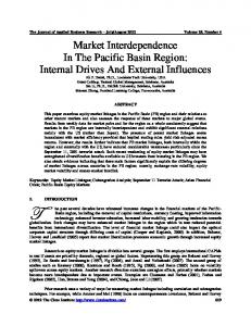
Referring to the break dates estimated by the LS test in Table 1, we allocate a level shift dummy (i.e., SBGD) ― as the deterministic component outside the cointegrating vector ― in each country’s cointegration analysis. For example, India’s SBGD of two breaks given by Model CC (SBCC) takes the form as illustrated in Fig. 1. The dummy variables reported in the forth column of Table 2 are chosen from the total of four allocations for each country and confirmed as optimal in estimating each model of different weakly exogenous variables (i.e., FOP, TOP and FST) 18 . Here, the selection mainly depends on whether the dummy allocation provides a single cointegration (r = 1) and no serial correlation in estimation.

16

The main argument given by Lee and Strazicich (2003; 2004) is that ADF-type endogenous break unit root tests exhibit size distortion and consequent spurious rejection of the null hypothesis when those tests are applied to unit root processes subject to break(s). Note that we stay away from this ongoing debate because the purpose of using the LS test in this analysis is to correctly set break dates in EG series. Hence, for confirming unit root/stationarity of each underlying variable, we conventionally rely on both ADF and PP tests (see Section 5.1). 17 As suggested by Lee and Strazicich (2003; 2004), we omit models B and BB of “changing growth” that assume break(s) in a trend only, since most economic time series can be adequately described by four models of A, AA, C and CC. 18 As far as the lag length is concerned, the effective lag order is selected for each model (see Section 5.1).


65



Table 1: Break Dates in EG Series India Indonesia Mexico Break date(s) Break date(s) Break date(s) A 1997Q1 1998Q1 1994Q2 AA 1992Q4,1997Q1 1991Q4,2001Q4 1993Q1,1996Q1 C 1997Q1 1998Q1 1996Q1 CC 1991Q4, 2004Q2 1995Q2,1998Q3 1994Q3, 1998Q3 Notes: Models A and AA = the clash models (break(s) only in the intercept); Models C and CC = the trend break models (break(s) in both the intercept and trend). Model

Fig. 1: India’s SBCC (= SBGD of Two Breaks Estimated by Model CC)

2 1 0 2008Q4

2004Q2

1991Q4

1981Q1

Table 2: Selected Lag Order (k), Deterministic Component and Dummy Variables Panel A: India Weakly exogenous variable k D. component Dummy variable FOP 3 Restricted trend SBCC, PCD TOP 4 Restricted trend SBAA FST 5 Restricted trend SBCC, PCD Panel B: Indonesia Weakly exogenous variable k D. component Dummy variable FOP 4 Restricted trend SBAA TOP 5 Restricted trend SBA FST 4 Restricted trend SBAA Panel C: Mexico Weakly exogenous variable k D. component Dummy variable FOP 5 Restricted trend SFD TOP 4 Restricted trend SBCC FST 5 Restricted trend SFCD Notes: SBA = SBGD of one break estimated by Model A; SBAA = SBGD of two breaks estimated by Model AA; SBCC = SBGD of two breaks estimated by Model CC; PCD = Pre-crisis dummy (one for 1990Q1 to 1990Q4 otherwise zero; only for India). SBC (= SBGD of one break estimated by Model C) is not selected.

5.

EMPIRICAL RESULTS

The total of 27 models was estimated for the three countries over different sample periods ― 1981Q1 to 2008Q4 for India, 1981Q1 to 2006Q4 for Indonesia and 1987Q1 to 2008Q4 for Mexico ― due to data availability. Nonetheless, during these periods, high economic growth and rapid financial deepening were typically observed together with liberalization in both the financial and trade sectors and severe financial crises in the three countries. While some models exhibit the evidence of heteroscedasticity and non-normality in residuals, all the models are free from serial correlation at the 10% significance level or better 19.

19

For conserving space, all the results relevant to the analysis are not presented (e.g., diagnostic and unit root tests) but are given on request.

66


International Business & Economics Research Journal – December 2011 5.1


Unit Root and Cointegration Tests

As the initial step in the cointegration analysis, both the Augmented Dickey and Fuller (ADF) (Said and Dickey, 1984) and Phillips and Perron (PP) (Phillips and Perron, 1988) unit root tests were conducted. The test statistics reveal that all the underlying variables of EG, FD, FC, FOP, TOP and FST are non-stationary in their levels but become stationary after taking the first difference. Thus, we conclude that these variables are I(1)20. Next, the Johansen (1988) cointegration test is implemented while FOP/TOP/FST is treated as a weakly exogenous variable in the cointegrating vector21. In performing the Johansen test, the effective lag order ― rather than the optimal lag order given by the lag section criteria ― is adopted for each model (see the second column of Table 2). For seeking the “effective” lag order, we check whether a lag order gives a single cointegration (r = 1) and autocorrelation-free significant estimates. Moreover, as the deterministic component, each of restricted intercept, unrestricted intercept and restricted trend is included into the cointegrating vector, and it is confirmed that the restricted trend provides best significant results to all the models (see the third column of Table 2); we empirically consider the trend component as a proxy for miscellaneous exogenous factors in each economy. Then, the trace statistics in Table 3 show that there is a single cointegration relationship (r = 1) among EG, FD and FC at the 5% level in all the models. Table 3: Johansen Cointegration Test Results (Trace Statistics) Weakly exogenous variable FOP TOP FST Null Result 5% Result 5% Result 5% r=0 73.253* 52.748 67.902* 54.575 55.319* 53.648 r