Advanced aircraft flight control using nonlinear inverse dynamics. X.-D. Sun. T. Clarke. Indexing terms, Aircraft fright control, Nonlinear techniques, Inverse ...
Advanced aircraft flight control using nonlinear inverse dynamics X.-D. Sun T. Clarke
Indexing terms, Aircraft fright control, Nonlinear techniques, Inverse dynamics
Abstract: A series of studies concerning the control of aircraft using nonlinear inverse dynamics based control techniques is presented. Following a summary of the inverse dynamics control theory, a design procedure for effective use of the method for flight control is generated. The novel features of the design have included the direct incorporation of handling qualities specification in the controller synthesis, the special considerations necessary for the inclusion of flap like direct force control devices (e.g. spoilers), and the introduction of ‘principal controller’ design for the efficient synthesis of multimode control systems using NID control. Detailed derivations of the symbolic inverse dynamics of the aircraft are given. The end result is a flight control system which satisfies handling qualities requirements and comprises mission-defined control modes for active control of the aircraft using nonlinear spoilers. Its success and effectiveness are demonstrated through simulation.
1
Introduction
The aerodynamic characteristics and operational requirements of modern high performance aircraft have forced greater consideration of increasingly intensive and complicated nonlinearities [I] within the system behaviour and control. The nonlinearities resident in the force and moment generation processes of an aircraft with strong, multiaxis, highly coupled features, may also be well associated with its flight operations. Some anticipated operational capabilities, i.e. supermanoeuvreability [2], require that aircraft be precisely controlled over a substantial portion of the flight envelope that encompasses strongly nonlinear aerodynamics and loss of control effectiveness. Clearly, for dealing with these strong nonlinearities, nonlinear control strategies are required which are based directly on the nonlinear model and which explicitly take into account the nonlinearities during the system synthesis process. In the design of flight control systems, these are expected to provide more effective control and the eficient utilisation of control resources.
‘c, IEE, 1994 Paper 15XOD (CX. C9), first received 24th January and in revised form 141h September 1994 The authors are with the Department of Electronics, University of York, York YO1 5DD. United Kingdom 418
There has been a great deal of progress in recent years in applying differential geometrical control theory to the linearisation and control of a nonlinear system. The theory has been relatively well developed and understood 131. As an important part of the theory and applications, the nonlinear inverse dynamics methodology [4] presents an equivalence to state space linearisation control using nonlinear coordinate transformations based on design of some ‘output’ functions [SI, and has attracted wide attention for its effectiveness and success in nonlinear flight control. Early studies in this area were connected with system decoupling and separation of control modes of aircraft [7, 8, 91. Use of the method for an aircraft with complex characteristics and operational requirements, such as the power lift STOL and V/STOL was carried out by Meyer et al. [IO]. During the same period, Wehreud et al. [ I l l applied the method to the control and testing of an aircraft flying through a large portion of the flight envelope. Later in 1984, Meyer et al. 1121) employed the method for the development of a helicopter control system, giving details of the construction of the transformation from the nonlinear system to the linear system. The latest works in this area include that of Lane and Stengel [I33 who applied nonlinear inverse dynamics to the development of a flight control system for a 12-state nonlinear aircraft model, with the major efforts on the effective control of the severe nonlinear effects from extreme flight conditions, such as high angle-of-attack and angular rates, and the research of Hauser et al. [I41 on the modified use of the method for the control of a non-rninimum phase nonlinear aircraft system. However, due to the complex modelling of aircraft auxiliary control devices, typically flaps and spoilers, their features and their unexpected effects on the invertible dynamics [lo], use of them for the active control of aircraft and, therefore, direct incorporation of them into control synthesis, based on nonlinear inverse dynamics, do not seem to have been studied before. Also, there is the clear need to develop a simplified, systematic and effective design routine for the practical use of nonlinear inverse dynamics for aircraft flight control. This paper describes a study that encompasses these considerations. Following a summary of the inverse dynamics control theory, a design procedure for effective use of the method for flight control is generated. The novel features of the design include the direct incorporation of a handling qualities specification in the controller synthesis, the special considerations necessary for the inclusion of flap like direct force control devices (e.g. spoilers [I 5 3 , and the introduction of ‘principal controller’ design for the development of multimode control I E E Proc -Control Theory A p p l . , Vol. 141, No 6 . November 1904
systems using NID control. A detailed derivation of the inverse dynamics of a combat aircraft is given in which a uniform derivative order is defined and applied to each of the principal control variables. The end result is a decoupled, multimode flight control system design for the aircraft, aiming to enhance its manoeuvrability and performance levels. 2
NID control: A brief summary
Generally speaking, the methodology is based on the following description of a nonlinear system:
with state variable x E W", control input ui E W,output A, b i , c are assumed smooth. It uses variable y E 9"'. input-output linearisation through the construction of the inverse dynamics, by differentiating the m (number of control) elements of the output y. A linear control is then designed using the linearised system and applied to the original nonlinear system through the inverse dynamicsbased transformation. The inverse dynamics of a nonlinear system (eqn. 1 ) are constructed by differentiating the individual elements of y with respect to time a sufficient number of times, e.g.
output) linear system:
[';I Y',"
(6)
=[U;]urn
with the ith output being controlled solely by the ith input. Necessary and sufficient conditions for the existence of local and global transformations for eqn. 1, which is equivalent to finding any A*(x) and the nonsingular B*(x) in eqn. 4, were obtained in the studies of Su [16] and Hunt et al. [17]. Unfortunately, for most modern dynamics systems with increased scale and complexity, the verification of the linearisability, strictly in accordance with the necessary and sufficient conditions, has proven a complicated and time-consuming routine [12]. However, it was shown that, when only the sufficient condition is considered, a much easier and more practical way of verifying linearisability for the nonlinear system in the form of eqn. 1 is the use of so called block lower triangular form [lo], which takes the following form:
i =
[
AI(X1, x2)
y!; -L2cj+
cLbLL2-'cj)ui j = 1, ..., m
(2)
I=,
where LA c j stands for the ith Lie derivative of the output y j with respect to A(x). For i = 1, L,cj = V(cj)A denotes the (scalar) directional derivative of y j along the direction of the vector A(x). The process continues until the smallest integer k is found such that at least one of the control inputs ui appears in y r , i.e. until at least one of the 'cj)ui# 0. The integer k is called the relative order for the output y j , denoted by r j . Clearly, it is dependent on both the system dynamics and the definition of the output variable. Define the transferring vector A*(x) and the decoupling matrix B*(x) as
]+[;I
Az(x13xz>x3) ..., xx) AAxi, ~ 2 . .,., xx)
A , - , ( x , , xz,
(7)
BAx)
The system is strictly m-axis in the sense that the dimension of x , equals rn for all integrator columns j from 1 to k so the system dimension is n = rn x k . B, is nonsingular and rn by m. Moreover, the block lower triangular form can conveniently be generated by judicious choice of output and control variables in the aircraft modelling process for N I D control purposes. A later design will demonstrate this. Once linearisation has been achieved, linear design methods, such as pole placement and linear modeltracking, can be applied. The model-tracking problem for the linearised system (eqn. 6) can be formulated by making use of the input: ui
=
y:;
+ ail(y:z:
I
-
L'a- ' C j )
+ . + q,,(ymi- y i ) ' '
A*(x) = [ L : c l ]
i = 1,
LYC, and
L,,(Ly'c,)
B*(X) =
[
.'.
:
LI,(Lp-1C,)
'
';I
Lbm(Ly1c1)
i "
(3)
0I =
y"r n l
+
Lb*(L'A"-lC,)
+ ail(y:il ' '
-
+ air, I ( j r n l ~
YY') - Li)
+ ai,,(y,i
- Yi)
i = 1, ..., m
Then eqn. 2 can be written as
I"]
= A*(x)
+ B*(x)u
(4) 0. I = 0. 8rn
If B*(x) E W"""is bounded away from singularity, the state feedback control law can be expressed through the following inverse dynamics formula: (5)
where U is the reference input. Substitution of eqn. 5 for the U in eqn. 4 yields the closed-loop decoupled (inputI E E Proc.-Control Theory Appl., Vol. 141, No. 6, November 1994
(9)
So the control for the linearised system, u i , can be decomposed into
y',"
U = - B*(x)- '(A*(x)- U)
..., m (8)
where ymi is the ith desired model output and the a,j are the characteristic polynomial coefficients. In the case of accurate system modelling, L>-'c, = yI'- I , yielding
+ c'.8fb
(10)
+
+
+
+
a , , y:; where uim = y:i . . a,,, , j m , ai,, y,, is defined as the output of a desired model and uifb = - ail y:' 1 - . . . - air,- ]ji- air,yi is the feedback needed for the pole-assignment of the closed-loop linearised system. Fig. 1 shows the model tracking mechanism. Substitution of ui into eqn. 6 with eqn. 9 yields ~
-
++aile:-'
+ . . . +a i r c e i = O
f o r i = 1, ..., m
(11) 419
where e, = y,, - y,. Thus asymptotic model-tracking can be obtained when the desired model output and its derivatives, y,,, j , , , . . ., f ; , : ' ( i = 1, . . ., m). are bounded and
b-
desired model generator
Fig. 1
linear equivalent plant
Model trackingfor the linearised system
all the poles, defined by s" in the left-half plane [SI.
3
+ ails"- + . . . + a,r,= 0, are
have normally been ignored, deleted or used with imposed constraints in the control synthesis. This is mainly because, for these applications, such devices were considered as being only occasionally used and/or weakly coupled, and the incorporation of such direct force generators as these might result in a system which is not invertible. Clearly, when these control devices are available and in active principal use, such arguments are not valid and may result in improper or even illogical control of an aircraft. In practice, for longitudinal control where flaps/ spoilers are in principal use, if the pertinent control vari= [V y a (or e)] and the ables are defined as the set control devices are the elevator, thrust throttle and spoilers, and where the spoiler model takes the general [20], the block nonlinear form C,, = K , , L(a) sin (a), lower triangular form required, based on the output set, can be found using the following procedure: (a) Introduce the nonlinear spoiler model into the aircraft model by augmenting the aircraft system dynamics with the first derivative of the spoiler control input (the deflection angle asp).6,, then becomes a new state variable driven by the input uaP(Asp = -asp 6,, + aspusp)(see Fig. 2). The corresponding first-order lag represents the spoiler actuator dynamics, which can be expected to have a high bandwidth (e.g. asp= 40.0).
Modelling of nonlinear aircraft for NID control
appropriate aircraft model can be obtained by assigning the lateral-related variables to zero, giving %
= q - q, = 4
1 mV
- - ( L - mg
cosy)
where V is the flight path velocity, a is the incidence angle, y is the trajectory elevation angle, q is the pitch angle (e) rate, q, is the wind-axis pitch angular rate. D, L and M represent the drag, lift and pitching moment acting on the aircraft, and are nonlinear functions of the aerodynamic coefficients and of the system variables ~191. To obtain the nonlinear form as eqn. 1 for NID control design, an appropriate transformation is required. This can be accomplished by augmenting the system dynamics with derivatives of appropriate control inputs. However, in the interest of forming a well-behaved block triangular system, special measures should be taken. In most previous studies concerning nonlinear flight control using the NID-based feedback linearisation methodology, control devices such as spoilers and flaps 420
S ' B
1
c, %qh(a)sin(+
(b) Define a first-order lag model for the jet-engine dynamics (e.g. a, = 0.5) so that the system dynamics may also be augmented by the first derivative of the thrust control 6,. This gives 8, = -a, 6, + a, U , (see Fig. 2). This is also demanded by matching the relative order of V with respect to the spoiler control. (c) Let U , = 6,. The above procedure produces a complete longitudinal open-loop aircraft system, having the following twodimensional three-axis block lower-triangular form, from which stable inverse dynamics can be constructed for the NID control laws:
where
I E E Proc.-Control Theory Appl., Vol. 141, No. 6, November 1994
and
- - D_
In the case of B(x)* being nonsingular, the controller is given by eqn. 5. Here, the coefficients of the designed closed-loop characteristic polynomial, defined by in eqn. 10, for each decoupled output variable are chosen by referring to handling qualities specifications MILF-8785C [21]. Table 1 lists the typical data for the output control variables V, y. 0 and a.
g sin y
m
( L - mg cos y) mV 4-Y M -
Table 1 : Pole polynomial Coefficients
I,, -a1
-asp
6,
Output variable Y
a,, u , ~
4,
V
5.0 3.0 3.0 3.0
1
Y
e
a
and U,, U, and uSpare the control inputs for 6,, 6, and 6,, , respectively. 4
NID flight control synthesis
4.1 New design approach for NID controller synthesis The nonlinear inverse dynamics control synthesis is applied to the system model (eqn. 13) to generate nonlinear controls. During the process, we developed a unique and efficient design procedure for the generation of various mission-defined controllers. For aircraft control, most output variables of interest can be, or approximately be, expressed as
These coefficient assignments define desired closedloop systems with relative stability qualities that meet the Level 1 specifications [21]. In the flight path, angle (y) channel, for example, the coefficient assignment gives ( r y = 2, from eqn. 9): "y
then from eqn. 6 : Y = -a,1d
-
ay,?
+
(17)
"ym
or, in transfer function form urn
(18)
+ a,:s + ay2
_ .
(14)
where C is a time-invariant (m x n) output matrix. This provides some simplification for the formation of multimode nonlinear controls and for the development of an efficient procedure and program package for the synthesis of a variety of the mission-defined controllers. Combined with the system modelling (eqn. 13) and the definition of output control variables, the major steps involved in the controller development are: (a) Put the control output variables of interest into the form y = C x , where C is a ( m x n) constant output matrix and y is chosen from the output control variable set y, . Here, for the longitudinal control
(16)
= Uym - ayld - ay27
= s2
y =cx
4.0 4.0 4.0 4.0
which corresponds to a second-order system with the natural frequency w, = 2 rads) and a damping ratio [ = 0.75 which give Level 1 Handling Qualities for the short period dynamics of the aircraft. The model reference terms U,,, (y,, and ym,) are formed by a desired model generator, which has the reference input y,,, from a trajectory command generator and takes the form:
p,,
Ymy
+ dmy, Lm, + dm72 Y m y = Y o ,
(19)
So, if d,,, and dmY2are taken to be the same as a,] and a v 2 ,as previously illustrated, we have
Y~ = [ V , Y, a, 8, q, 4,&I'
(b) Calculate the derivatives
or y(s) = y,,(s),
in order to obtain the inverse dynamics matrices. For the model of eqn. 13 and the output control variable set above, ri = 2 was used for x i and ri = 1 was for x 2 . (c) Design multimission-defined controllers by simply assigning the output matrix C according to mission objectives and the control dimension m, and performing the following computations to the transferring vector and the decoupling matrix needed: A(x):,
1
=
"[E
B(x):,, = C [ ;
(Ly1x)].4(x); (L>-lx)]B(x)
I E E Proc.-Control Theory Appl., Vol. 141, No. 6, November 1994
which shows the desirable model tracking in the case of precise system modelling and control. Note that the delay in the servodynamics (typically in the elevator and the thrust channels) and the nonlinearities, caused by saturations in both the amplitude and rate of the control inputs, were not included in the model (eqn. 12). Appropriate and separate adjustments in the coefficients of vim (desired model) and (feedback control) in eqn. 10 for improved tracking of the trajectory command input are necessary and suggested. 4.2 Application of NID to advanced aircraft flight control 4.2.1 Definition of a set of principal control variables: The above design procedure was applied to the development of a longitudinal NID flight control system for a 421
combat aircraft [19]. For systematic programming and efficient controller synthesis, a set of principal output control variables was defined which had the same dimension as the output variables of interest, and from the derivatives of which, controllers for those sets of output variables can be easily generated. According to the modelling of the longitudinal dynamics (eqn. 13), the principal control variables are chosen as y, = x I = [Vya]’. The nonlinear controller corresponding to this output vector was developed upon the computation of the second-order Lie derivatives, the symbolic forms of which are derived as following. 4.2.2 First Lie derivatives of the principal control variables: The first Lie derivatives of the principal control
variables can be easily formed from the aircraft dynamics equations:
3 au =
-
(tpV2S
2 + cr x,
6, sin u ) / m
a v-0 aq
av_ - C,,,
cos ajm
as,
a ax
a’
-(LA(y))=-= ax
[a’- a’ ay a’
av
]
(26)
]
(27)
a’ a’ as,,
- -
ay aa aq ad,
where
-(D + mg sin y)
where the lift and drag are modelled as
and H and M are height and Mach number, respectively. If the inputs are defined as those in eqn. 12, we get
L,,((L: y,)
=0
fori
=
1, 2, 3
(22)
4.2.3 Second Lie derivatives of the principal control variables: According to eqn. 2, the second-order Lie
derivatives of the principal control variables can be expressed as
_ ” -- C ,
mclx
86,
sin a/mV
3= (i P V Z S
as,, -((L a ax
(a))=-= A
ax
”.as,,. )ymV [av
ai ai ae ae aci ai a y aa aq as, ad,,
where, in longitudinal control, ci
= q - 9.
Therefore
and
aaqi -- 1.0, _
-ai =
ah,
-3 -aias,’ as,,
-
--ay
as,,
A key step is to find the Jacobian 4.2.4 Design of the principal controller: The trans-
ferring vector A:(x) and the decoupling matrix B f ( x ) for the principal output variables are defined as Since y, = [ V , y, U ] ’ , we need (a/ax)(LA(V)),(ajax)(LA(y)) and (a,0x)(LA(a)),which are given by
av -
av
av av av av av
-
ay aa
aq as, as,,
and
where
a t_ _- 9 ay 422
In the case of Bf(x) non-singular, the feedback controller for the principal variables is given by cos y
up = ( B f ( x ) ) - ’ ( u- A f ( x ) )
(29)
I E E Proc.-Control Theory Appl., Vol. 141, N o . 6, November 1994
o,o av a v
av
av _ av _ _ av ay aa
can be synthesised as
as, as,,
ay ay ay a j ay - - - 0.0 - av ay aa as, as,,
B:(x) =
ai _ ai _ adr _
ai
ai
av
av
86,
assp
0
- a, -asp
0
-a,
ay
ai
as,
a, as, -
ay
as,,
- a,
(30)
ay
as, as,,
-
[ V , 01’
adr a6,,
asp
ak ay as,, as,
1 11 In this case, the spoiler is treated as a state variable so only the sub (2 x 2) matrix in B: will be used for the system inverse, giving the controller: U =
B:(x)-’(u - A:(X))
(34)
Clearly, this mode can also be used as a back-up mode to which the full dimensional controller will be switched when there is a failure in spoiler control or an occurrence
So, the inverse dynamics of the aircraft with rn = 3 will be unsolvable when: (a) a, aspbaa(x)= 0; control device saturation or it ceases working. For individual cases (elevator or thrust or spoiler), the controller will automatically be switched to one of the reduced-dimension modes discussed next. (b) The relation between the spoiler control and the thrust control fulfils:
ak
= 2, y, =
A: = C, A: B: = C , B: with 1 0 0
-
86,
bab)
Controller three: rn
0 [ba,(x)
a ~ a~.p-_ ;
_ a v ay a@
=
0 0
_I
(32)
From eqns. 24 and 25, eqn. 30 can be expressed as
defined by, and connected with, the choices of the groups of the output control variables and the controllers as described above. According to these, Table 2 summarises some major control modes designed for the longitudinal flight control of the aircraft, with class A for conventional control and class B for unconventional control. Modes A1 and A2 are designed for conventional control augmentation in aircraft velocity and attitude while B1 B4 are the control modes utilising spoilers, or similar direct force devices, for some unconventional control purpose. The mission objectives for which a control mode is expected to be applicable are listed in the right-hand column of the Table.
-
Tabla 2: Lonaitudinal control m o d e summary
(33) During the online control computation, the above relationship is checked by the program at each time step, in conjunction with the computation of eqns. 25 and 26. As the singularities appear, the control system will automatically adopt a basic control mode (e.g. controller three in Section 4.2.6) using the conventional controls U, and U,. 4.2.6 Design of multimode controllers: After defining the inverse dynamics for the principal output variables, controllers in the form of eqn. 5 for other sets of output y, can easily be constructed. variables given by y = C , , Here are some examples. Controller one: m A: = CIA:
B:
=
3, y1 = [ V , y, 01’
= CIB,*
with
Controller two: rn
A:
=
A:
B:
=
=
3, y,
=
[ V , y, a]’
B:
IEE Proc.-Control Theory Appl., Vol. 141, N o . 6, November 1994
Control mode
Outout control variables
Mission obiectives
A(m=2) A1 A2
[vel [Vu1
cruising conventional trajectory manoeuvring
B (m-3) B1
[evi
62
[VYSI
unconventional levelflight decelerating. gust/turbulence alleviation, takeoffpanding unconventional fixed y, (I manoeuvring unconventional fixed 0. (I manoeuvring
For the implementation of the control system on a fly-by-wire system, these control modes will be constructed through different data bases and program routines so they are flexibly switched from one to another according to different flight mission objectives and system performance requirements. 4.3 System configuration The complete principal configuration of the longitudinal inverse dynamics flight control system (LIDFCS) is shown in Fig. 3. The N I D control was incorporated within a previously designed nonlinear flight simulator for the aircraft, where the online N I D control computation included the selection of controllers according to 423
mission command
1 I
control mode
Ln8=
I
-
model generator fmg(Ycm)
Ycm
model tracking reference
Ym c
vm
~
PACL 8 NI0 Matrices
t
A*(x) B * ( x )
1
I I U
w disturbance input
1
system linearisation
secvodynomics
= (B*(x)) (v-A*(x))
aircraft
6
(longitudinal dynamics)
6:f*d(b,u)
x
z
f
(x.6 w
ff,(Y.Y)(ff,(Lp,
)
I
I I
PACL 8 feedback controller Y.Y))
I I
pole assignment
_ _ _ _ _ _ - _ _ Fig. 3
-1
LIDFCS configuration
It is considered that the robustness of NID flight control is of great importance: firstly, the effectiveness of a desired N I D control is heavily dependent on the modelling accuracy of the dynamical system to be controlled. This is, in principle, due to the need for an exact cancellation of all nonlinear terms for the valid implementation of designed linear control laws. Secondly, it has become increasingly difficult to model precisely most modern technology and high performance aircraft with increased dynamic ranges, flight envelopes, nonlinearities and aerodynamics. Under these considerations, a control algorithm based on an adaptive control logic [22] for robustness enhancement of the NID control was investigated and it was later incorporated within the LIDFCS.
Evaluation of LIDFCS: flight control
of decoup,ed
Combined with the study into the applications of the various active control schemes for advanced aircraft, the
designed LIDFCS was thoroughly evaluated by the manoeuvring of an aircraft under NID control of the system. The mission was to control the aircraft along a flight trajectory containing both conventional and unconventional manoeuvres. The trajectory, shown in Fig. 4, involves successive phases of climb, fuselage pointing (pure pitch control with flight trajectory fixed), and level-attitude descent. The control programming was made by matching the control mission with the longitudinal control modes shown in Table 3. According to the mission, three of the modes, (i) the conventional V-a manoeuvring (control mode A2), (ii) the decoupled V-y-0 manoeuvring (control mode B2) and (iii) the V-a-0 manoeuvring (control mode B4), were selected and then linked successively by the LIDFCS to form the required mode-shifting control. Table 3 also contains a detailed summary ofthe flight simulation broken down into 10 s manoeuvre blocks. The effectiveness and benefits are apparent: following the programmed mode-shifting control, the LIDFCS commanded the logical deflections and changes of the control
Table 3:Simulation summary Seg. no. Time, s
Control mode
Output variables
V(rn/s)
vf")
UP)
er)
H
189-199 199-189 189 189 189
0-11.8 11.8-0
0
0-1 1-4 4-8
01.12.8 12.8-4 4-8
0--6
0-6
8-0
ox-3
0-3
0
500-710 710 710 710-530 530 400
~
1 2 3
424
0-10 10-20 20-30 30-40 40-53
A2 62 62 64 84
-
IEE Proc.-Control Theory Appl., Vol. 141, No. 6, Nooember 1994
devices (Fig. 4d, e) and gave precisely decoupled control of the output variables of interest (Fig. 4a, b), and, therefore, enhanced the aircraft manoeuvrability. The fuselage pointing manoeuvre enhances the air-superiority of a
2001 phase 1
8001 E.
fighter during combat, and improves attitude handling and augmentation during landing. The direct force manoeuvre (flight trajectory control with fixed attitude), as shown in phase 3, considerably improves the
phase 3
phase 2
600-
4oo-
climb phasel
300
phase 2
phase 3
I
0
I
I
I
I IO
20 I
30 I
40I
50 I
60 I
50
60
1.5
C
I
0
I
I
I
I
I
I
10
20
30 1.5
40
50
60
'1
phasel
0
IO
phase 3
phase 2
20
30
40
t .5
b
d
phase2
phase 3
Fig. 4 Simulotion of decoupledflight control Flight trajectory in H-X plane
Y
b Decoupled control of angularvariables
c Control of flight path velocity d Elevator and thrust control outputs e Spoiler control output
I E E Proc.-Control Theory Appl., Vol. 141, No. 6, November 1994
425
manoeuvrability of a modern aircraft and is useful for flight missions such as mid-air refuelling, formation flying, take off/landing and air-superiority. 6
Concluding remarks
A series of studies are discussed in this paper on the design of advance flight control for modern high technology aircraft using the nonlinear inverse dynamics methodology. The successful development of the NID flight control system for an aircraft demonstrates that the NID method is effective for synthesising nonlinear controllers to achieve complex and mission-defined control objectives, and for generating a decoupled, multi-mode control system for aircraft. Combined with the system development, a number of new techniques for more efficient use of the N I D method for flight control have been studied. These include the direct incorporation of the handling qualities specification of aircraft into the desired model dynamics and into the characteristic polynomials, and the introduction of a novel controller synthesis procedure for the generation of a multimode flight control system, featuring the use of a set of principal output control variables (principal controller) and an uniform relative degree choice for all the control modes of interest, for utilising active spoiler control. The system development work has proven these techniques to be effective and successful. 7
References
I HUANG, C.Y., and KNOWLES, G.J.: ‘Application of nonlinear control strategies to aircraft at high angle of attack‘. Proc. of the 29th IEEE Conference on Decision and Control, WA 8, Dec. 1990. 2 HERBST, W.B.: ‘Future fighter technologies’, J. Aircraft, 1980, 7 , (E), pp 561-566 3 ISIDORI, A.: ‘Nonlinear control systems’ (Springer Verlag, 1989) 4 AKHRIF, O., and BLANKENSHIP, G.L.: ‘Using computer algebra for design of nonlinear control systems’. Thesis Report M.S. 87-2, University of Maryland, 1987.
426
5 SASTRY, S., and ISIDORI, A.: ‘Adaptive control of linearizable systems’, IEEE Trans., 1989, AC-34, pp. 1123-1131 6 McLEAN, D.: ‘Automatic flight control systems’ (Prentice-Hall, 1990) 7 SINGH, S.N., and RUGH, W.J.: ‘Decoupling in a class of nonlinear systems by state variable feedback‘, AIAA J. Dynamics Syst. Means. Control, 1972, pp. 323-329 8 ASSEO, S.J.: ‘Decoupling of a class of nonlinear systems and its application to an aircraft control problem’, AIAA J. Aircraft. 1973, 10, pp. 739-747 9 FREUND, E.: ’Decoupling and pole assignment in nonlinear systems’, Electron. Lett., 1973, 9, pp. 373-374 10 MEYER, G., and CICOLANI, L.: ‘Application of nonlinear system inverses to automatic flight control design - system concepts and flight evaluations’. AGARDograph 251 on Theory and applications of optimal control in aerospace systems, 1981, paper 10 I I WEHREND, W.R., Jr., and MEYER, G.: ’Flight tests of the total automatic flight control system (TAFCOS) concept on a DHC-6 twin otter aircraft’. NASA TP-1513, 1980 12 MEYER, G., SU, R., and HUNT, L.R.: ‘Application of nonlinear transformations to automatic flight control’, Automntica, 1984, 20, (l), pp. 103-107 13 LANE, S.H., and STENGEL, R.F.:‘Flight control design using nonlinear inverse dynamics’, Automatica, 1988, 24, (4), pp. 471-483 14 HAUSER, J., SASTRY, S., and MEYER, G.: ‘On the design of nonlinear controllers for flight control systems’, A I A A Paper No. 893489-CP, 1989. 15 MACK. M.D., SEETHARAM, H.C., KUHN, W.G., and BRIGHT, J.T.: ‘Aerodynamics of spoiler control devices’, A I A A 1979, paper 19-1843 16 SU, R.. ’On the linear equivalents of nonlinear systems’, System & Control Lett., 1982, 2, p. 48 17 HUNT, L.R., SU, R., and MEYER, G.: ‘Global transformations of nonlinear systems’,IEEE Trans., Control, 1983, AC-28, p. 24 18 ETKIN, B.: ‘Dynamics of atmospheric flight’ (John Wiley, 1972) 19 HERD, J.: ‘Digital simulation techniques for a fixed-wing aircraft’. 3rd year report, Dept. of Aeronautics, Imperial College, London, 1985 20 SUN, X.D.: ‘Active control of aircraft using spoilers’. PhD thesis, Imperial College, University of London, 1993 21 MOORHOUSE, D.J., and WOODCOCK, R.J.: ’Background information and user guide for MIL-F-878% military specification flying qualities of piloted airplanes’. AFWAL TR-81-3109, 1982 22 SUN, X.D., WOODGATE, K.G., and CLARKE, T.: ‘Adaptive control for the robustness enhancement of advanced inverse dynamics flight control systems’. Proc. 1st Asian Control Conference, 1994, 2, pp. 449-452
IEE Proc.-Control Theory Appl., Vol. 141, No. 6 , November I994