Advanced Partitioning Techniques for Massively Distributed Computation Jingren Zhou
Nicolas Bruno
Wei Lin
Microsoft
Microsoft
Microsoft
[email protected]
[email protected]
ABSTRACT An increasing number of companies rely on distributed data storage and processing over large clusters of commodity machines for critical business decisions. Although plain MapReduce systems provide several benefits, they carry certain limitations that impact developer productivity and optimization opportunities. Higher level programming languages plus conceptual data models have recently emerged to address such limitations. These languages offer a single machine programming abstraction and are able to perform sophisticated query optimization and apply efficient execution strategies. In massively distributed computation, data shuffling is typically the most expensive operation and can lead to serious performance bottlenecks if not done properly. An important optimization opportunity in this environment is that of judicious placement of repartitioning operators and choice of alternative implementations. In this paper we discuss advanced partitioning strategies, their implementation, and how they are integrated in the Microsoft Scope system. We show experimentally that our approach significantly improves performance for a large class of real-world jobs.
Categories and Subject Descriptors H.2 [Information Systems]: Database Management
Keywords Scope, Partitioning, Distributed Computation, Query Optimization
1. INTRODUCTION An increasing number of companies rely on the results of massive data computation for critical business decisions. Such analysis is crucial in many ways, such as to improve service quality and support novel features, to detect changes in patterns over time, and to detect fraudulent activities. Usually the scale of the data volumes to be stored and processed is so large that traditional, centralized database system solutions are no longer practical or even viable.
Permission to make digital or hard copies of all or part of this work for personal or classroom use is granted without fee provided that copies are not made or distributed for profit or commercial advantage and that copies bear this notice and the full citation on the first page. To copy otherwise, to republish, to post on servers or to redistribute to lists, requires prior specific permission and/or a fee. SIGMOD Š12, May 20–24, 2012, Scottsdale, Arizona, USA. Copyright 2012 ACM 978-1-4503-1247-9/12/05 ...$10.00.
[email protected]
For that reason, several companies have developed distributed data storage and processing systems on large clusters of thousands of shared-nothing commodity servers. Examples of such initiatives include Google’s MapReduce [5], Hadoop [1] from the open-source community and used at Yahoo, and Cosmos/Dryad [3, 12] at Microsoft. In the MapReduce approach, developers provide map and reduce functions in procedural languages like C++, which perform data transformation and aggregation. The underlying runtime system achieves parallelism by partitioning the data and processing each partition concurrently using multiple machines. This model scales reasonably well to massive data sets and has sophisticated mechanisms to achieve load-balancing, outlier detection, and recovery to failures, among others. This approach, however, has its own set of limitations. Users are required to translate their application logic to the MapReduce model in order to achieve parallelism. For some applications this mapping is very unnatural. Users have to provide implementations for the map and reduce functions, even for simple operations like projection and selection. Such custom code is error-prone and hardly reusable. Moreover, for complex applications that require multiple MapReduce stages, there are often many valid evaluation strategies and execution orders. Having developers manually implement and combine multiple MapReduce functions is equivalent to asking them to specify physical execution plans directly in relational database systems, an approach that became obsolete with the introduction of the relational model over three decades ago. Moreover, optimizing complex, multi-step MapReduce jobs is difficult, since it is not usually possible to do complex reasoning over sequences of opaque, primitive MapReduce operations. To address this problem, higher level programming languages plus conceptual data models were recently proposed, including Jaql [2], Scope [3, 24], Tenzing [4], Dremel [15], Pig [18], Hive [21], and DryadLINQ [23]. These languages offer a single machine programming abstraction and allow developers to focus on application logic, while providing systematic optimizations for the distributed computation. These optimizations take advantage of a full view of the application logic, and can perform sophisticated query optimization strategies that are simply not possible otherwise. In massive distributed computation, data shuffling is typically the most expensive operation and can lead to serious performance bottlenecks if not done properly. A very important optimization opportunity in this type of environment is that of judicious placement of repartitioning operators and choice of different implementation techniques. Com-
plex scripts and reasoning about properties of intermediate results opens the door to a rich class of optimization opportunities regarding data partitioning. It is crucial to avoid repartitioning unless absolutely necessary, and do so as efficiently as possible. Previous work focused on minimizing the number of partitioning operations while executing complex scripts [24]. However, independently on how much we optimize input scripts, there are still scenarios that require data shuffling. There are also different ways to perform data shuffling, and each one is preferable under different conditions. The optimal choice of shuffling operations depends on many factors, including data and code properties, and scalability requirements. It is valuable to integrate the reasoning with the query optimizer and systematically consider alternatives with the rest of the query. In this paper we describe advanced partitioning techniques that leverage input data properties and optimize data movement across the network. As a result, we are able to greatly improve the shuffling efficiency, by either avoiding unnecessary repartitioning or partially repartitioning the input data set. The techniques are applicable both at compilation time and at runtime. We also design a novel partitioning strategy which indexes intermediate partitioned results and stores them in a single sequential file. This approach fundamentally solves the scalability challenge for data partitioning and efficiently supports an arbitrarily large number of partitions. All the partitioning techniques are implemented into the Scope system at Microsoft, which is running in production over tens of thousands of machines. The query optimizer of Scope considers different alternatives in a single optimization framework and chooses the optimal solution in a cost-based fashion. Experiments show that the proposed techniques improve data shuffling efficiency by a few folds for real-world queries. Although this paper uses Scope as the underlying data and computation platform, the ideas are applicable to any distributed system that relies on a query optimizer and performs data shuffling. The rest of the paper is structured as follows. In Section 2 we review the necessary technical background to support the remaining sections. In Section 3 we describe the implementation of partial repartitioning and its interaction with the query optimizer. In Section 4 we discuss a scalable index-based partitioning strategy. Section 5 reports an experimental evaluation of our strategies discussed on realworld data. Section 6 discusses related work, and Section 7 concludes the paper.
2. PRELIMINARIES Scope [3, 24] (Structured Computations Optimized for Parallel Execution) is the distributed computation platform for Microsoft’s online services targeted for large scale data analysis. It incorporates the best characteristics of both MapReduce and parallel database systems. The system runs over large clusters of tens of thousands of machines, executes tens of thousands of jobs daily, and it is on its way to become an exabyte store. We start with an overview of Scope, including the query language, query optimization, and different partitioning types. The reader can find more details on these concepts in the literature [3, 24, 12].
2.1 Query Language The Scope language is declarative and intentionally reminiscing SQL. The select statement is retained along with
joins variants, aggregation, and set operators. Like SQL, data is modeled as sets of rows composed of typed columns, and every rowset has a well-defined schema. At the same time, the language is highly extensible and is deeply integrated with the .NET framework. Users can easily define their own functions and implement their own versions of relational operators: extractors (parsing and constructing rows from a raw file), processors (row-wise processing), reducers (group-wise processing), combiners (combining rows from two inputs), and outputters (formatting and outputting final results). This flexibility allows users to solve problems that cannot be easily expressed in SQL, while at the same time is able to perform sophisticated reasoning of scripts. Figure 1(a) shows a very simple Scope script that counts the different 4-grams of a given single-column string data set. In the figure, NGramProcessor is a C# user defined operator that outputs, for each input row, all its n-grams (n = 4 in the example). Conceptually, the intermediate output of the processor is a regular rowset that is processed by the SQL-like main query (note that intermediate results are not necessarily materialized between operators at runtime).
2.2
Query Compilation and Optimization
A Scope script goes through a series of transformations before it is executed in the cluster. Initially, the Scope compiler parses the input script, unfolds views and macro directives, performs syntax and type checking, and resolves names. The result of this step is an annotated abstract syntax tree, which is passed to the query optimizer. Figure 1(b) shows an input tree for the sample script. The Scope optimizer is a cost-based transformation engine based on Cascades framework [9], and generates efficient execution plans for input trees. Since the language is heavily influenced by SQL, Scope is able to leverage existing work on relational query optimization and perform rich and non-trivial query rewritings that consider the input script in a holistic manner. The Scope optimizer extends Cascades by fully integrating parallel plan optimization and performing more complex structural data property reasoning, such as partitioning and sorting of intermediate results. The optimizer returns an execution plan that specifies the steps that are required to efficiently execute the script. Figure 1(c) shows the output from the optimizer, which defines specific implementations for each operation (e.g., streambased aggregation), data partitioning operations (e.g., the repartition operator), and additional implementation details (e.g., the initial sort after the processor, and the unfolding of the aggregate into a local/global pair). Finally, code generation produces the final algebra (which details the units of execution and data dependencies among them) and the assemblies that contain both user defined code and runtime implementation of the operators in the execution plan. Figure 1(c) shows dotted lines for the two units of execution corresponding to the input script. This package is then sent to the cluster, where it is actually executed. Users can monitor the progress of running jobs, and there are management utilities to submit, queue, and prioritize scripts in the shared cluster.
2.3
Data Partitioning
A key feature of distributed query processing is based on partitioning data into smaller subsets and processing partitions in parallel on multiple machines. This requires opera-
Output (output.txt)
Global Stream Agg ({ngram}, count)
SV2 Repartition (ngram)
Output
Local Stream Agg
(output.txt)
({ngram}, count)
Aggregate ({ngram}, count)
Sort (ngram)
SV2 Process
Process
SV2
SV2
SV1
(NGramProcessor)
(NGramProcessor)
Get
Get (input.ss)
SV1
SV1
SV1
SV1
SV1
(input.ss)
(a) Scope script
(b) Input tree
(c) Output tree
(d) Scheduled graph
Figure 1: Definition, Compilation, and Scheduling of a Simple Scope Script tors for splitting a single input into smaller partitions, merging multiple partitions into a single output, and repartitioning an already partitioned input into a new set of partitions. This can done by a single operator, the data exchange operator, that repartitions data from n inputs to m outputs [8]. After an exchange operator, the data is partitioned into m subsets that are then processed independently and in parallel using standard operators, until the data flows into the next exchange operator. Exchange is implemented by one or two physical operators: a partition operator and/or a merge operator. Each partition operator simply partitions its input while each merge operator collects and merges the partial results that belong to its result partition. Suppose we want to repartition n input partitions, each one on a different machine, into m output partitions on a different set of machines. The processing is done by n partition operators, one on each input machine, which read its input and split it onto m local partitions, and m merge operators, one on each output machine, which collect the data for their partition from the n corresponding local partitions. Figure 1(d) shows five partition operators at the end of each SV1 vertex instance split their input into three partitions each, and three merge operators at the beginning of each SV2 vertex instance merge the five pieces of a corresponding partition.
where there is a single input stream that is partitioned into m streams, without merge operators. Finally, Full Merge (Figure 2(c)) is a special case of full partitioning when there is a single output stream, merged from n input streams without partition operators. In this paper we explore alternative implementations of exchange operators that are based on additional topologies.
2.3.2
An instance of a partition operator takes one input stream and generates multiple output streams. It consumes one row at a time and writes the row to the output stream selected by a partitioning function applied to the row in a FIFO manner (so that the order of two rows r1 and r2 in the input stream is preserved if they are assigned to the same partition). There are several different types of partitioning schemes. Hash Partitioning applies a hash function to the partitioning columns to generate the partition number to which the row is output. Range Partitioning divides the domain of the partitioning columns into a set of disjoint ranges, as many as the desired number of partitions. A row is assigned to the partition determined by the value of its partitioning columns, producing ordered partitions. Other non-deterministic partitioning schemes, in which the data content of a row does not affect which partition the row is assigned to, include round-robin and random. The example in Figure 1(c) uses hash partitioning.
2.3.3 (a) Full Repartitioning (b) Initial Split
(c) Full Merge
Figure 2: Different Types of Data Exchange
2.3.1 Exchange Topology Figure 2 shows the main classes of exchange operators. Full Repartitioning (Figure 2(a)) consumes n input partitions and produces m output partitions, partitioned in a different way. Every input partition contributes to every output partition, resulting in n · m connections. In the example of Figure 1(c), the plan uses full repartitioning on the nGram column in SV1, so that the input, which is not partitioned by nGram, can be aggregated correctly by SV2. Initial Split (Figure 2(b)) is a special case of full partitioning
Partitioning Schemes
Merging Schemes
An instance of a merge operator combines data from multiple input streams into a single output stream. Depending on whether the input streams are sorted individually and how rows from different input streams are ordered, we have several types of merge operations. Random Merge randomly pulls rows from different input streams and merges them into a single output stream, so the ordering of rows from the same input stream is preserved. Sort Merge takes a list of sort columns as a parameter and a set of input streams sorted on the same columns. The input streams are merged together into a single sorted output stream. Concat Merge concatenates multiple input streams into a single output stream. It consumes one input stream at a time and outputs its rows in order to the output stream. That is, it maintains the row order within an input stream but it
does not guarantee the order in which the input streams are consumed. Finally, Sort-Concat Merge takes a list of sort columns as a parameter. First, it picks one row (usually the first one) from each input stream, sorts them on the values on the sort columns, and uses the row order to decide the order in which to concatenate the input streams. This is useful for merging range-partitioned inputs into a fully ordered output. In the example of Figure 1(c), the different partitions are ordered by nGram due to the sort operator, so we use the Sort Merge variant to ensure the right row ordering when consumed by the global stream aggregate operator.
2.4 Job Scheduling Scope relies on Dryad [12] to schedule the compiled script inside the cluster. The execution of a script can be modeled as a graph, where each vertex represents an instance of a computation unit, and each edge corresponds to data flow between vertices 1 . Figure 1(d) shows the execution graph for the sample script, assuming that the input data is laid out in five machines and the optimizer determines that data would be better aggregated into three partitions. Vertex scheduling is rather sophisticated and takes different factors into consideration when deciding which vertices to run next, and on which machine to place such vertices (e.g., data locality, average execution time and memory consumption). Additionally, the nature of the graph imposes some natural scheduling constraints. A vertex can only start when all its inputs are already finished processing. For instance, in Figure 1(d), any SV2 vertex can only begin after all SV1 vertices finish. This is required not only to avoid producers and consumers running concurrently, but also because we need to simultaneously Sort-Merge SV2’s inputs.
2.5
Structured Streams
In Scope, structured data can be efficiently stored as structured streams. Like tables in traditional databases, a structured stream has a well-defined schema that every record follows. Additionally, structured streams can be directly stored in a partitioned way, which can be either hashor range-based over a set of columns. Data in a partition is typically processed together (i.e., a partition represents a computation unit). Each partition may contain a group of extents, which is the unit of storage in Scope. In the example of Figure 1(c), data is read from a structured stream input.ss, which is not partitioned by nGram (and therefore a repartition operator is needed). If the input structured stream were partitioned by nGram already, the resulting plan would consist of a single computation unit SV1, on which the final partitioning operator is replaced by the output operator. Relying on pre-partitioned data significantly reduces latency by removing both the data exchange and the superfluous global aggregate operators.
2.5.1
Indexes for Random Access
Within each partition, a local sorting order is maintained through a B+ -Tree index. This organization not only allows sorted access to the content of a partition, but also enables fast key lookup on a prefix of the sorting keys. Such support is very useful for queries that select only a small portion of the underlying data, and also for more sophisticated strategies such as index-based joins. In our example, if input.ss were partitioned and sorted by nGram, we could not only remove SV2 as explained earlier, but also the sort operator in SV1, with an additional improvement in performance.
2.4.1 Aggregation Trees Vertex scheduling attempts to minimize the overall job latency. One important aspect to achieve this goal is to reduce recovery costs due to failures. Consider a merge operator that consumes data from a very large number of partition vertices (i.e., suppose in Figure 1(d) that there are a thousand SV1 partition vertices connecting to each one of the three SV2 vertices). The chance of a random failure in SV2 while reading SV1 outputs increases with the number of input connections. Moreover, any such failure causes the whole SV2 vertex instance to restart, wasting partial work. To alleviate this problem, aggregates are typically done using aggregation trees, which can be seen as checkpoints during aggregation. When the number of input connections to an aggregate vertex is beyond a certain limit, we introduce partial aggregate vertices that operate over fragments of the input partition vertices. This works well for queries where merge operations interact with algebraic partial aggregation, which reduces the input size and can be applied multiple times at different levels without changing query correctness. We can then aggregate the inputs within the same rack before sending them out, reducing the overall network traffic among racks. As an example, if the threshold is 250 input connections and we have a thousand SV1 instances in Figure 1(d), for each one of the three SV2 instances, we would introduce four partial aggregate vertices, each working on one fourth of the SV1 instances, based on the network topology. 1 To simplify the presentation, we do not discuss mechanisms that dynamically expand or contract the graph at runtime.
2.5.2
Data Affinity
Scope does not require all the data that belongs to a partition to be stored in a single machine. Instead, Scope attempts to store all the data in a partition close together by utilizing store affinity. Every extent has an optional affinity id. All the extents with the same affinity id belong to an affinity group. The system tries to place all the extents of an affinity group on the same machine unless the machine has already been overloaded. In this case, the extents are placed in the same rack (or a close rack if the rack itself is overloaded). Each partition of a structured stream is assigned an affinity id. As extents are created within the partition, they get assigned the same affinity id, suggesting that they should be stored together. Processing a partition can be done efficiently either on a single machine or within a rack. Store affinity is a very powerful mechanism to achieve maximum data locality without sacrificing uniform data distribution. The store affinity functionality can also be used to associate/affnitize the partitioning of an output stream with that of a referenced stream. This causes the output stream to mirror the partitioning choices (i.e., partitioning function and number of buckets) of the referenced stream. Additionally, each partition in the output stream uses the affinity id of the corresponding partition in the referenced stream. Therefore, two streams that are referenced not only are partitioned in the same way, but partitions are physically placed close to each other in the cluster. This layout significantly improves parallel join performance, as data need not be transferred across the network.
3. PARTIAL DATA REPARTITIONING As described in Section 2.3, data partitioning typically consists of one or two physical operators: a partition operator, which splits its input into local partitions, and/or a merge operator, which collects and merges the local partitions that belong to the corresponding output partition. In absence of additional information, as illustrated in Figure 2, every merge vertex needs to connect and read data from every partition vertex. As we discuss in this section, however, by carefully defining the partition scheme of the exchange operator (e.g., number of partitions and partition boundaries), we can guarantee that certain local partitions would be empty. Additionally, we can somewhat influence how much data has to be transferred, and to which destination. This general approach has several advantages during execution. First, by carefully defining partition boundaries, we can drastically reduce data transfer between partition and merge vertices by taking data locality into account. Second, partition vertices need to reserve fewer memory buffers and storage due to local partitions that are guaranteed to be empty. Third, the job manager does not need to maintain explicit connection state between partition and merge vertices for which the local partitions are empty, which reduces the footprint of the scheduler. Fourth, merge vertices do not have to wait for all partition vertices to finish executing, but only for those that actually contribute to the corresponding partition. This is important because a single partition outlier can delay all merge vertices from starting, increasing overall latency. Finally, fewer input connections to merge vertices reduce the chance of failures, thus requiring fewer intermediate aggregates (see Section 2.4.1), which improves overall performance. In this section we explore efficient alternatives to perform data repartitioning that leverage properties of the input data to be repartitioned. Depending on the partitioning scheme, we discuss how to construct and implement data exchange operators that are defined over effective partitioning boundaries and only require a subset of connections between partition and merge vertices. Additionally, we discuss how to integrate these alternatives during query optimization. To illustrate the different partitioning techniques, we use the simple script below: SELECT a, UDAgg(b) AS aggB FROM SSTREAM "input.ss" GROUP BY a; OUTPUT TO SSTREAM "output.ss" [HASH | RANGE] CLUSTERED BY a;
The input in the script is a structured stream distributed in the cluster. The script performs a user defined aggregation UDAgg on column a and outputs the result into another structured stream, either hash- or range-partitioned by a.
3.1 Hash-based Partitioning We consider the case in which the script writes a structured stream hash-partitioned by column a. We assume hash partitioning is done by first applying a hash function to the partitioning columns and then having the hash value modulo the number of output partitions to generate the partition number to which the row goes. As long as the hash function and the number of output partitions are fixed, hash partitioning is deterministic.
Output (output.txt)
Stream Agg ({a}, UDAgg(b))
SV2 Repartition (a)
SV1 Get (input.ss)
Figure 3: Execution Plan for a Simple Script Figure 3 shows an execution plan for the script. Assuming that the input is not already partitioned by column a, the plan reads the input in parallel and hash-repartitions the data on column a (SV 1 in the figure), and then merges the partitions, performs the user defined aggregate and outputs the result (SV 2 in the figure). Note that in our example UDAgg is not associative nor commutative, so we cannot use local/global aggregates as in Figure 1(c)). If the input were already partitioned by a, a different execution plan without repartitioning would be preferable (i.e., read each partition, perform the aggregation, and write results in parallel). Output (output.txt)
SV3 Repartition SV1 (a,50)
SV2 Stream Agg ({a}, UDAgg(b))
Repartition (a,200)
SV1 Get (input.ss)
Figure 4: Partial Hash Repartitioning Suppose that the input is indeed hash-partitioned by column a into 100 partitions. However, the user defined aggregate is very expensive, so we choose to repartition the input into 200 buckets. Additionally, the output of the aggregate is smaller than the input, so we choose to additionally repartition it into 50 buckets before the final output, in order to avoid writing too many small fragments. The resulting execution plan is shown in Figure 4. In principle, the execution plan looks rather expensive due to two full repartition operators. However, in this scenario there are important optimization opportunities. In fact, repartitioning a 100-way partitioned input into 200 partitions (by the same column) can be done by locally splitting each of the original partitions into two, without any network data transfer. Also, repartitioning a 200-way input into 50 partitions can be done by partially merging the input partitions. We next formalize this approach, and characterize when it is effective.
3.1.1
Determining Data Flow Connections
Suppose that we want to hash partition an input T into po partitions, and T is already hash-partitioned into pi partitions by the same columns. The naive execution plan contains pi vertices P0 , . . . Ppi−1 , each one partitioning its input into po local partitions, followed by po merge vertices
M0 , . . . , Mpo−1 , each one reading and merging the i-th local partition from each of the pi partition vertices. Interestingly, for certain values of pi and po, some local partitions in Pi vertices would always be empty and do not need to be read by Mj vertices. Example 1 Suppose that pi = 4 and po = 2 (i.e., we want to partition 2-ways an input that is already 4-way partitioned). Every row in P0 satisfies h(C) ≡ 0 mod 4, where h is the hash function and C are the partitioning columns. Figure 5(a) shows the default partitioning strategy which connects every input vertex with every output vertex. In this case, we know that h(C) ≡ 0 mod 2 as well, and therefore P0 would never generate a row satisfying h(C) ≡ 1 mod 2. Thus, M1 does not need to read the empty local partition produced by P0 . In general, M0 only reads from P0 and P2 , and M1 from P1 and P3 . Figure 5(b) shows the refined merge graph. A similar strategy can be applied when pi = 2 and po = 4. Figure 5(c) shows the refined partitioning graph.
M0
P0
P1
M1
P2
M0
P3
P0
(a) Full Partitioning
P1
M1
P2
M0
P3
M1
P0
M2
M3
P1
(b) Partial Merge (c) Partial Partitioning
Figure 5: Different Hash Partitioning Strategies In general, merge vertex Mi (0 ≤ i < po) needs to read from partition vertex Pj (0 ≤ j < pi) if there might be a row in Pj for which its hash value modulo po is i. In other words, if there exists an integer k such that k ≡ j mod pi and k ≡ i mod po. By definition, this implies that there are integers k1 and k2 such that k = k1 · po+i and k = k2 ·pi+ j, and therefore k1 · po + i = k2 · pi + j, or po · k1 + (−pi) · k2 = (j − i) This is a linear diophantine equation of the form a·x+b·y=c, which has integer (x, y) solutions if and only if c is a multiple of the greatest common denominator of a and b. In our case, there are solutions, and therefore Mi needs to reads from Pj if and only if (j − i) is a multiple of gcd(po, −pi), or, more concisely, if and only if i≡j
mod gcd(pi, po)
If pi and po are co-primes, then gcd(pi, po) = 1 and the optimized technique is the same as the traditional one (i.e., we need to connect every partition and merge vertex instances).
3.2 Range-based Partitioning The ideas in the previous section can also be applied to range partitioning scenarios. Consider again the script in the previous section when it writes a structured stream rangepartitioned by column a. Suppose now that the input in the figure is range-partitioned by columns (a, b). Note that this property does not imply the data being partitioned by a alone, since two rows that share a values might be in different partitions due to varying b values. In this case, the same plan of Figure 3 can certainly be used, with a full repartitioning on a. However, an input that is range-partitioned by (a, b) can be repartitioned by a in a cheaper way by locally splitting and merging the original partitions, as shown next.
P1=[(1,A)…(1,C))
P2=[(1,C)…(2,E))
P3=[(2,E)…max)
1,A 1,A 1,B 1,B
1,A 1,A 1,B 1,B
P’1=[1…2)
1,C 1,D 2,A 2,D
1,C 1,D 2,A 2,D
P’2=[2...3)
2,E 3,A 3,B 4,A
2,E 3,A 3,B 4,A
P’3=[3…max)
Figure 6: Refining Range Partitions from (a, b) to a Example 2 Consider the data set at the left of Figure 6, which is range-partitioned by columns (a, b) into three partitions. Partition P2 , for instance, contains all rows with values in the interval [(1, B), (2, D)) (note that the interval is closed on left and open on right). As shown in the figure, we can repartition this data set by column a without connecting each partition output with each merge input. The precise connectivity map can be statically computed at compile time given the original partitioning boundaries. Note that the output partition P1′ receives data from input partitions P1 and P2 . While P1 is fully contained into P1′ , we need to filter rows in P2 with a < 2 to avoid incorrect results. Compared to the initial physical partitions Pi , we call Pi′ as logical partitions, each of which conceptually reads one or more physical partitions with optional filtering predicates. The end result is that Pi′ is range-partitioned on column a. In general, partial range-based repartitioning can be applied whenever the input and output partition schemes share a common column prefix (otherwise, there is no choice but to connect each partition vertex with every merge vertex). The general approach consists of two steps. First, we need to determine the range boundaries for each output partition. With this information, we can then generate code that determines the output partition for each incoming row, and determine which partition and merge vertices are connected. We next discuss these steps in detail.
3.2.1
Determining Partitioning Boundaries
The main goal of query optimization is to minimize the resulting job latency. In the context of range partitioning, and especially with respect of boundary determination, there are two main aspects that contribute to overall latency. First, the resulting partitions need to be evenly distributed. Any skewed partition is likely to introduce outliers during execution, as a partition that is significantly larger than the average increases the latency of the overall job (and likely propagates skewed partitions to subsequent execution vertices). Second, the cost of the repartitioning operator itself is important, which is directly proportional to the amount of network data transfer. As a consequence, we should try to align input and output partition boundaries as much as possible. This way, we avoid splitting input partitions in multiple large fragments that are sent across the network. Suppose that we want to repartition data on columns C, where each partition is roughly of size T . When the input is already partitioned by columns C ′ (where C and C ′ share a common prefix), the input partitioning metadata information itself can be viewed as a (coarse) histogram B over
columns C ′ , with each partition representing a bucket in the histogram2 . We assume that buckets maintain the number of rows that are included in its boundary, that bucket boundaries are closed on left and open on right, and that the last range on right is a special maximum value that is larger than any other valid value. The information from such histograms can help the system choose partition boundaries. Some very common column types (e.g., strings or binary columns) are not amenable to interpolation, which limits what we can infer about value distributions inside a histogram bucket. Specifically, in this case we know all bucket boundaries but we cannot interpolate and generate intermediate values within input buckets. Under this natural restriction, Algorithm 1 describes a greedy approach to determine partition boundaries that are compatible with C and would result in partitions of size around T . Algorithm 1: PartitionBoundaries(C, T, B) Input: Columns C, Partition size T, Buckets B Output: Partition boundaries P /* Assume that C and B.cols share common prefix CP and for each 1 < i