(PIE) that support the dynamic evolution of processes. .... Looking at the software process literature, the first observation with respect to the ..... to the company.
Advanced Services for Process Evolution: Monitoring and Decision Support Ilham Alloui1, Sami Beydeda2, Sorana Cîmpan1, Volker Gruhn2, Flavio Oquendo1 and Christian Schneider2 1
University of Savoie at Annecy, ESIA LLP, 41 avenue de la Plaine B.P. 806, 74016 Annecy Cedex, France {alloui,cimpan,oquendo}@esia.univ-savoie.fr 2 University of Dortmund, Computer Science Department, Software Technology, 44221 Dortmund, Germany {beydeda,gruhn,schneider}@ls10.cs.uni-dortmund.de
Abstract. Process support environments (PSEs) are widely used for modelling, enacting and analyzing human intensive processes. The benefits of a PSE become apparent when processes to be supported are long lived and distributed and contain heterogeneous components. Generally, such processes are subject to dynamic evolution, i.e. they have to be changed during their execution. Unfortunately, virtually none of the existing PSEs consider dynamic evolution of processes. This article explains the concepts and techniques underlying a set of components developed in the ESPRIT Project Process Instance Evolution (PIE) that support the dynamic evolution of processes. These concepts and techniques are demonstrated using a real-world scenario from the automotive industry.
1
Introduction
Generally, processes1 are embedded in real-world environments such as a company producing goods for a particular market. As indicated by the saying “the world is changing”, every real-world environment is subject to evolution which implies the evolution of the embedded processes. For instance, change in market requirements could trigger the evolution of the company process to produce goods that have more appropriate properties. The process support environment (PSE) used by an organization for the effective management of its processes has also to consider the evolution of these processes. This means that the PSE has to provide not only guidance and automation of tasks, but also it has to maintain the evolution of the processes it supports. An evolution support component should therefore be integrated into any PSE. Evolution support offers controlled mechanisms for: • identifying the need for process evolution; • determine evolution alternatives and select one alternative to implement; 1
An exact definition of the used terminology can be found in [15, 24].
• implement the selected alternative. In the PIE project [13, 28], these tasks are addressed by different components; monitoring support (MS), decision support (DS) and change support (CS). The evolution strategy support (ES) handles the overall strategy employed by the evolution process [18]. The objective of MS is mainly to identify the process-internal reasons for process evolution. The reasons for process evolution can be classified into two main groups: process-internal and process-external. A process-internal reason for process evolution can be for example an unacceptable value for the observed progress of the process, i.e. the process manager could decide to modify a process that cannot meet the deadlines. Furthermore, the MS within the PIE framework possesses proactiveness. Proactiveness refers to the ability of identifying trends. The process manager should be informed not only about a process that has already been delayed, but also whether a process will be late in the future. After identifying the need to evolve a process, the next tasks concern the generation of solutions and the evaluation of these solutions. The DS component assists the process manager in carrying out both tasks. The process manager can request the component to generate alternative modifications of a single process instance, or the underlying process model. She then has to decide which modification to carry out. In both cases, the DS component provides support in exploring and evaluating the alternatives. Based on probability distributions of throughput time and total costs, the component determines the alternative with the highest utility for the process manager. After exploring appropriate alternatives, the next task of the process manager is to implement the most promising alternative. The objective of the CS component within the PIE framework is to provide the project manager with detailed information about the implementation of a particular modification. The information provided should help the project manager maintain consistency in the modified process instance. For example, if the project manager has decided to skip an activity in order to improve throughput time, CS has to assist the manager in connecting predecessor to successor activities. However, this article is focused on MS and DS, this means we do not consider CS. This article explains in detail MS and DS. Section 2 introduces a case study from the automotive industry, which is used to demonstrate the applicability of the various concepts. Section 3 explains the concepts underlying MS. The concepts underlying DS are described in section 4. Section 5 presents a scenario related to the case study proposed in section 2. This scenario can be used to highlight some of the functionalities of the MS and DS. Finally, section 6 contains our conclusions.
2
Case Study
The case study we will use throughout this paper is currently used in the PIE project, and is taken from the automotive industry [14]. It relates to (part of) the process of designing a sport variant of an existing car. The output of the process is a CAD representation of the new sport variant. It is a process that involves creativity and an
extensive use of computer means. This characteristics make it similar to a software proces. For the part of the process we are interested in, there are three departments involved in the development of the new sport variant: the style department, the body-in-white2 department and the packaging department. The style department provides sketches of the hood for the sport variant, based on the hood of the existing car platform. The body-in-white department modifies the hood design, starting from the previous designs and the sketches from the style department. The outcome of their work is the hood design for the sport variant, a CAD version. The packaging department checks the integration of the hood design with its environment, i.e. the other elements of the body design such as the headlights. Each of the departments follows its own process in order to provide its outputs. We do not detail the processes followed by the style and design departments, but regarding the packaging department, that part of the integration tests that concerns the fitness of existing headlights with respect to the new hood design is described. A scenario linked to this case study is presented in section 5.
3
Monitoring Support (MS)
The need for measuring processes and analyzing the data collected on them is by now accepted and the Capability Maturity Model [21] with its forth and fifth maturity levels (“managed” and “optimized”) offers a suitable methodological framework to do it. We present in this section a MS and its underlying modelling formalism. The section is organized as follows: section 3.1 presents the related work with respect to the monitoring issue, section 3.2 presents the monitoring approach while section 3.3 presents an example of monitoring analysis, the conformance factors. 3.1
Related Work
Looking at the software process literature, the first observation with respect to the monitoring issue is that the scope and the features are very broad. All studied cases use certain means for data collection, but the analyzes made on collected data as well as the scope are very different. The analyses employed vary from no analysis at all, as is the case in the Hakoniwa system [22] to the use of statistics and probability [7,11,12] and classification trees [31]. With respect to the scope, the monitored processes vary from short term repeatable processes in which case analyses are made on the entire process, as in the Balboa system [11], to long term and complex processes in which only parts of a process are 2
Body-in-white (BIW) designates in automobile companies the subdivision of the design office that designs the external shape of the vehicle from specifications issued by the styling department.
monitored, as is the case in the monitoring prototype experiment undertaken at the AT&T Bell Laboratories [7]. 3.2
Monitoring Approach
All the mentioned systems make the assumption that precise and certain information is available for collection. The prototyping experiment has some means for handling imprecision in the form of granularity (measurements are made on a daily basis, even though finer grain information would give a more accurate information). This approach is meant to reduce experiment costs and to make it less intrusive. The need for precise information increases the costs of data collection, thus limiting the usage of the monitoring system that becomes too costly and intrusive. In this context, the existence of a monitoring mechanism that handles imprecise and uncertain information would reduce the costs of monitoring and would increase its acceptance, as it would be less intrusive. The monitoring mechanisms proposed in this paper use fuzzy set theory [32,33] for representing the data, which allows expressing imprecise and uncertain information. Of course the system handles precise data in the classical way, as fuzzy sets theory is an super set of the classical sets theory. The system architecture allows integration in a process support environment leading to a reduction of data collection costs, as most of such data can be automatically collected, without much interference in the subject process. The proposed monitoring is open to evolution, i.e. new analysis techniques can be added. This feature increases the flexibility of the support provided to the user. The monitoring system uses monitoring models maintained in a Model Library. We distinguish between different kind of models: • Basic model: this model allows to indicate what information to collect and what analyses or transformations to make on the collected data. The motivations behind the selection of a certain information to be collected is up to the modeler. A GQM approach can be used to decide what metrics to apply [5]. • Sensor model: indicates where from the data is to be collected. • Display model: indicates what information to display to the user. • Publication model: indicates what information to publish for the other components in the environment of the monitoring. • Trace model: indicates what information to trace, i.e. what information is to be kept for use in the future. For a given basic model, different sensor, display, publication and trace models may be defined for the integration in different environments. When the monitoring is launched, the models to be loaded are indicated. This component complies with the PIE Common Component Architecture which is described in [18]. A formalism for defining monitoring models has been developed in the PIE framework [8]. A detailed presentation of the formalism is out of the scope of this paper, only some characteristics of the formalism will be presented. The theory on which the formalism is based is the fuzzy set theory, which was developed by Zadeh in order to represent mathematically the imprecision related to
certain object classes [32,33,6]. It also responds to the need for representing symbolic knowledge, in natural language, subject to imprecision or presenting a vague character. A fuzzy subset A of a reference set X is characterized by an application from X to [0,1]. This application called membership function and noted µA allows to represent how much the elements x of X are also members of A. If µA(x)=1 the value x is completely a member of A and if µA(x)=0 it is not at all a member of A. In the particular case when µA(x) only takes values equal to 0 or 1, the fuzzy subset A is identical to a classical subset of X. The formalism provides means for the representation of numeric as well as symbolic information, in a precise and certain as well as imprecise and uncertain form. The formalism also provides operators to handle such type of information. Thus there are arithmetic operators for working with fuzzy numbers, meaning functions to pass from numeric to linguistic universes, aggregation tables for combining symbolic information etc. A presentation of this formalism can be found in [8]. The existence of a formalism for defining monitoring models makes the MS open to evolution. The formalism allows to define new monitoring models, thus new analysis techniques. The monitoring can also be used to monitor the monitoring of the subject process. This reflexive way of using the monitoring allows the tuning of the system [2,3]. Examples of tuning are the modification of fuzzy membership function and aggregation tables. In order to better illustrate the functional and operational aspects of the MS, we will present an analysis technique employed by the MS, namely the conformance factors [9,10]. This example also allows us to illustrate the use of the fuzzy sets theory.
3.3
Conformance Factors: an Analysis Technique
The conformance factor analysis technique is used in order to compare the conformance, for a given aspect, between the process enactment (what happens) and the process instantiation (or process plan, what is supposed to happen). Examples of aspects of the process are progress, cost, effort consuming, chance of success, etc. In the following we will illustrate the conformance factor related concepts using the progress aspect. Aspects can be associated with process attributes. Following [16], the measure of attributes values can be direct (corresponding to raw data collected by the monitoring) or indirect (corresponding to monitoring analyses results). Each of the attributes are represented under a given universe of discourse (domain). Such a universe may be numeric or linguistic. For the progress, the considered universe is linguistic, and contains the terms {missed, almost missed, extremely late, very late, late, slightly late, on schedule, slightly ahead, ahead, very ahead, extremely ahead}. This means that the progress of a process fragment will be expressed using these terms. The linguistic universes given as examples here are ordinal, but linguistic universes where an order is not defined can also be considered. For a considered attribute, a goal is set by the process manager indicating the values considered as target, i.e. what are the values one would like to observe during enactment. For the progress conformance factor, an example of goal is to be on
schedule. This is a restrictive goal, and fits processes where the deliver in time is the prior concern. A more relaxed one is to consider the goal as slightly late, on time or slightly advanced. The goals presented are crisp goals, as they represent classical subsets of their universe of representation. The goals may also be represented as fuzzy subsets of the universe. The observed value for an attribute is obtained by analyzing data collected from the actual process. Its expression is a (fuzzy) subset of the universe in which it is represented. For the above progress example, the observed progress is expressed in terms of membership degree to each of the linguistic terms. The progress is obtained as combination of two attributes: completeness (how much of the planned work is actually completed) and moment (the position in time with respect to schedule). These attributes are also linguistic, and their combination is made by means of symbolic aggregation [9,10]. By comparing the goal and the observed value for a given attribute, the corresponding conformance level is computed, its values being placed in the interval [0,1]. A value of 0 for the conformance corresponds to no conformance at all, while a value of 1 corresponds to total conformance. In addition, a threshold is set by the process manager for the acceptable level of conformance. An example of threshold may be 0.8. Every conformance level lower than 0.8 would then indicate an unacceptable deviation, and an alarm would be set by the MS. µLcompleteness 1
very low
low
medium
high
very high
0.8 0.2 0
20 22 30
40 45
55 60
70
80
100 NCompleteness
Fig. 1. Correspondence between numeric and linguistic universes of completeness using of meaning functions As mentioned earlier, the observed value for progress is calculated by means of symbolic aggregation between completeness and moment. The completeness has two universes of representation (see Fig. 1): • the interval [0,100]=Ncompleteness for a representation in terms of achieved percentage, • the linguistic universe LCompleteness composed by {very low, low, medium, high, very high} for a linguistic representation.
The membership functions indicated in Fig.1 are subject to tuning , in order to adjust them to certain context of use. Let us consider the process fragment in the design department for producing the new hood design (see section 2). If this process is monitored for progress, the design department would be systematically asked for the completeness of their work. Depending on the availability of this information, the design department can provide this data in a precise and certain form, for instance 22%, or in a imprecise manner, using the linguistic representation , for instance small or very small. If the value given by the design department is a linguistic one, it will be used as acquired in the symbolic aggregation in order to obtain the progress. If the data provided is a numeric one, the MS uses the meaning functions in order to pass from the numeric representation to the linguistic one. For the value of 22% the following linguistic representation is obtained3: µLcompleteness(22) = {0.8/very low, 0.2/low, 0/medium, 0/high, 0/very high}4
(1)
The interpretation of this result is that the value of 22%, and by that the completeness of the new hood design, can be described to certain positive degrees as very low and low. This linguistic representation is obtained using the membership functions in Fig.1. If the membership functions are changed (by tuning) then the results also change. The moment has also two equivalent representations; one in the interval [PlannedStartingDate, PlannedEndingDate] and one in the linguistic universe LMoment={very beginning, beginning, middle, end, very end}. The correspondence between the two universes is made by similar meaning functions. The moment corresponds to the elapsed time. The value of the progress attribute is obtained using the symbolic representation of completeness and moment. The observed value for progress obtained after the symbolic aggregation is a fuzzy subset of its universe of representation. The symbolic aggregation uses rules associated with a pair of linguistic terms (one from the completeness universe and one from the moment universe) from the universe of progress. An example of such a rule is the following: If completeness is low and moment is beginning then progress is on time
(2)
Starting from the membership degrees of the observed completeness and moment to the different linguistic terms of their corresponding universes, the observed progress is computed. The following formula is used in order to compare it with the user defined goal: C(goal, observedValue)=1-min{1, Σk max {µLk(observedValue)- µLk(goal),0} Lk∈LmonitoredAspect
(3)
When the membership degree of the observed value to some term is greater than the respective membership degree for the goal (indicating elements that are not 3
The observed completeness is represented as a fuzzy sub-set of the completeness linguistic universe 4µ Lcompleteness stands for the membership value
included in the goal sub-set), the difference is decreased from the maximum conformance value (1 in our case). The more the value of conformance is closer to 1, the more the actual behaviour of the process conforms to the defined goal, so the deviation is smaller. When the conformance is 1 there is no deviation and the enactment conforms to the process plan and the user-defined goals. Similar examples to the one for progress can be considered, for instance by combining the completeness and the effort. The progress example is a simple one, and it was chosen for illustrative purposes. The monitoring formalism allows to represent other types of analyses.
4
Decision Support (DS)
After identifying the need to modify a process instance or its model, the process manager has to carry out two tasks. Firstly, the process manager has to identify solutions to the problem identified by either MS or the user. Secondly, these solutions have to be analyzed with respect to their impact. Of course, the second task is only required when more than two alternatives, including the alternative of doing nothing, are available. The objective of the DS component within the PIE framework is to assist the project manager in carrying out these tasks. In this section, we present our approach for these two tasks. The structure of the section is as follows: section 4.1 gives a brief overview of the literature on decision and risk analysis, section 4.2 contains an approach for identifying alternative modifications to a process model while section 4.3 includes a description of the technique which is used to analyze a process instance and to determine possible changes to a process instance. 4.1
Related Work
Almost every decision problem is adhered with risk due to the uncertainty of the real world. Despite its importance, the term risk is not exactly defined and its interpretation depends on the context [17, 25, 23]. In the context of the PIE project, we interpret the notion of risk in accordance with Moskowitz and Bunn [26] as the likelihood of an unfavourable outcome. Researchers have long considered risk analysis and decision problems under uncertainty. Bernoulli and Bayes developed a formal framework two centuries ago which was further developed by Ramsey [30], von Neumann and Morgenstern [27], Arrow [4] and others. The method used within the PIE project is based on this formal framework. Unfortunately, in the context of process technology, risk and decision analysis have received little attention, and in the PIE project, we attempt to investigate approaches and techniques for those important issues.
4.2
Proposition of Alternatives
Levels of Modifications to a Process Generally, a process can be modified at two levels: the instances of the process model and the process model. For example, a process instance being too late in producing particular goods can be improved by providing each activity affecting the throughput time with additional resources such as manpower. By providing additional resources, the activities can be executed more effectively which generally leads to a decreased throughput time of the instance. The same objective can also be achieved by re-designing parts of the process model affecting the throughput time. The difference between these two levels of modifications is that a modification of the process model affects every instance generated after the modification, whereas a modification of an instance has no effect on subsequent instances. Specifically, single instances are often modified in cases where they deviate from the process model. Deviations of process instances from their corresponding models can be determined using the approach of Cook/Wolf [12]. We have two different approaches for identifying those alternatives that contribute to an improvement of the process. While changes to a single process instance can be determined using the technique for analyzing the process instances, changes to the process model require special considerations, as it is explained in the next subsection. Identifying Possible Modifications to the Process Model Generally, modifying a process at the level of its model requires semantic information. In the simplest case, the semantic information would have to include the importance of each activity. This would allow determining which of the activities could be skipped in cases of restricted resources and which one may not be skipped. One of the concerns in the PIE project is the integration of different PSEs that would support the subject process and would allow the independence of the system from the meta-model used by such PSEs. This is why we in PIE use a generic metamodel called common meta-model whose concepts are mapped to the ones used by different PSEs. Only the PIE evolution components have knowledge of the common meta-model, which is rather general and does not take into account any semantic information. Thus, modifications at this conceptual level can only be carried out by a human process manager. The process manager has to determine those modifications that are most likely to lead to the intended goal. After having determined alternatives, the process manager can use the analysis facilities provided by the DS component, which are explained below, to identify the most promising alternative. This cycle of determining and analyzing alternatives generally leads to a gain of experience. Fortunately, by storing this experience, the DS component could assist the process manager in finding possible solutions in the future. Modifications proposed by the process manager can be stored in a database, called experience database, together with the results of the analysis in order to reuse these solutions in similar situations. Therefore, some means are needed to determine the similarity of such situations. The methods used by the DS component employ the delta-analysis approach proposed by Guth and Oberweis [19] to compare the current situation with those occurred in the past. In the approach of Guth and Oberweis, two models are compared
to identify their differences. After having identified the differences between the two models, a ratio, called delta, is calculated. Two models are said to be similar if the corresponding delta value is below a particular threshold. Thus, in order to find similar models in the database maintained by the DS, the delta value is computed for each of the models in the database. Those models that have a delta value below the threshold are tested with respect to their applicability to the current situation using the analysis facilities provided by the DS component. 4.3
Analysis of Process Instances
As mentioned above, our technique for analyzing process instances can be used for two different tasks. Firstly, this technique is capable of identifying those activities that substantially contribute to the throughput time as well as to the total costs. Both the throughput time and the total costs can be improved by improving these activities. Thus, the proposed technique can be used for optimizing process instances. Secondly, the technique can determine probability distributions of the time and the costs of executing the process instance. These probability distributions can be used to compute simple risk measures such as the expected value and the variance [1] of the distribution or the more complex value-at-risk measure [23] used in the finance area. These measures can be used to compare a pair of alternatives. Representation of a Process Instance Our technique for analyzing a process instance operates on a representation of this instance as a graph with the following properties. Nodes in the graph represent activities of the process instance. Each node possesses two attributes. One of the attributes represents the costs of the resources required for the execution of the activity. The other attribute attached to a node represents the additional time needed to finish the activity under consideration. The graphical representation of a process instance also includes special nodes referred to as exit nodes. Exit nodes indicate the completion of the execution of the process instance. Control flows within the process instance are represented by edges connecting the nodes. Since an activity can have different outcomes and the succeeding activity may depend on the outcome, a node can have more than one outgoing control flow edge. In these cases, each outgoing edge is augmented with a probability to indicate the likelihood to take a particular branch. Obviously, the sum of the probabilities attached to the outgoing edges of one activity has to be exactly 1 and in the case of only one succeeding activity the probability attached to the edge corresponds to 1. In our approach, an instance of a process model is represented by a set including the currently executing activities. Each activity A in this set is attached with a parameter At indicating the time to finish. Thus, if T is the current time, a currently executing activity Ai will finish at time T+At. Activities which are not contained in this set are not executing and are considered to be idle. Each activity in the set of executing activities possesses two parameters. One of these parameters indicates the costs caused by the process prior to the execution of the activity. Note that this parameter does not include the costs incurred by the activity till the current time. The other parameter indicates the probability of entering the activity. Thus, the cost and
the probability parameters attached to an exit node give the corresponding values for finishing the process instance at that particular node. Algorithm processInstanceAnalysis; Input processModel; SetOfExecutingActivities; output processInstanceTimeSchedule; setOfWaitingActivities; begin T=currentTime(); setOfWaitingActivities={}; while setOfExecutingActivities not empty do for all activities A ready to start in setOfWaitingActivities do delete A in setOfWaitingActivities; insert A in setOfExecutingActivities; determine that activity A in setOfExecutingActivities finishing next; delete A in setOfExecutingActivities; instId=AinstId; for all B in setOfExecutingActivities do Bt=Bt-At; T=T+At; mt=T; if A is an exit node of processModel then mc=Ac; mp=Ap; put m in processInstanceTimeSchedule; for all successor S of A in processModel with Sp*Ap>pthres do Sc=Sc+Ac; Sp=Sp*Ap; SinstId=instId; instId=newInstId(); if SinstId ≠ AinstId then for all B in setOfExecutingActivities with BinstId=AinstId do C=copy B; CinstId=SinstId; put C in setOfExecutingActivities; for all B in setOfWaitingActivities with BinstId=AinstId do C=copy B; CinstId=SinstId; put C in setOfWaitingActivities; if all resources and products are available for the execution of S then put S in setOfExecutingActivities; else put S in setOfWaitingActivities; if processModel does not contain a successor S of A with Sp*Ap>pthres then for all B in setOfExecutingActivities with BinstId=AinstId do delete B in setOfExecutingActivities; for all B in setOfWaitingActivities with BinstId=AinstId do delete B in setOfWaitingActivities; return (processInstanceTimeSchedule, setOfWaitingActivities); end
Fig. 2 Algorithm for analyzing process instances
Determination of the Process Instance Time Schedule The next step in our analysis involves the elaboration of a process instance time schedule. A process instance time schedule is a set consisting of marks which indicate the end of an activity execution. Besides, there are special marks indicating that the entire process instance has finished, i.e. the last activity of the process has finished. These special marks are attached with the total costs and also with the probability to finish at that time. The algorithm for generating the time schedule is given in figure 2. The basic idea of the algorithm consists of considering every possible execution thread of the process instance simultaneously. Starting with the set of executing activities characterizing the process instance under consideration, the currently concluded activity is deleted from the set of executing activities and its succeeding activities are inserted, depending on the availability of the required products and resources, in the set of executing or waiting activities. Each time an activity is deleted from the set of executing activities, a mark indicating this event is inserted in the time schedule. If the entire process instance is finished, the mark then includes information concerning the total costs and the probability of that event. After finishing the execution of an activity, the set of waiting activities is searched for activities that have become ready to start, i.e. the required products and resources have become available. This loop is executed until the set of executing activities is empty i.e. there are no possible threads of execution in the process instance. A non-empty set of waiting activities indicates a deadlock situation. The probability attached to each activity in the non-empty set gives the likelihood of the particular deadlock situation. Computation of Probability Distributions and Risk Measures The output of the above explained algorithm, i.e. the time schedule for a particular process instance, can be used to determine the probability distribution of both the throughput time and the total costs of the instance. In order to obtain the probability for a particular time or cost value, the time schedule is queried for that value. If the time schedule contains several entries with this particular value, their probabilities are summed up to compute the probability of this value. After having identified a probability distribution, statistical measures can be used to define appropriate risk measures. As mentioned above, the expected value and the variance [1] of the distribution or the more complex value-at-risk [23] defined on the basis of the distribution can be used as risk measures. Based on such risk measures, a utility function [29] can be defined taking into account the preferences and the risk aversion of the process manager. Thus, selecting an alternative involves computing the utility of all the available alternatives and then selecting that alternative which dominates all the others. Process Instance Optimization The results of the algorithm can be used for three kinds of optimizations. Firstly, the set of waiting activities of an optimal process instance should always be empty. Generally, a waiting activity indicates that by synchronizing predecessor activities the throughput time of a process instance can be decreased. Secondly, optimizations can be achieved by analyzing the set of executing activities. A process instance can be effectively improved with respect to the throughput time and total costs by improving
those activities that appear frequently in the set of executing activities. Thirdly, the parameters of a process instance which determine the shapes of the probability distributions for throughput time and total costs are known. Thus, the shapes of these probability distributions can be formed as intended by altering these parameters. Specifically, this optimization can be automated if symbolic expressions are computed for the various probabilities.
5
Illustrative Scenario
This section presents a scenario and illustrates how the evolution support presented in this paper is used. The scenario is related to the case study presented in section 2, and deals with the study of a design variant that causes a “deviation process” to be put in place [14]. Let us consider that the Body Design Manager (BDM) is monitoring the Body Design process in terms of progress. The MS raises an alarm. Although the process deadline has not been reached yet, using its proactive features the MS observes that the process is likely to be late. BDM requires the MS component to provide more information about the progress and state of the composed sub-processes, i.e. the packaging and the hood design processes. The data given by the monitoring component indicates that the progress of both sub-processes corresponds to late and there is a clash issue in the packaging process. A clash is associated to an unexpected situation, that might imply the blocking of the process, some rework or supplimetary work to be made. An inquiry made by the BDM reveals the problem: although the specification for the new hood was that the shape of the headlights should not change, digital mock-up shows that this is not the case. The front shape of the headlights fits perfectly with the external part of the hood, but this is not the case internally, where the rear part of the headlight now interferes with the new hood shape. This clash corresponds to a rework, as the design of the hood has to be remade. Given the situation in the body design process, i.e. the process is late and there is a clash issue, the BDM launches the DS asking for alternatives. The DS uses simulation techniques to identify those activities within both sub-processes whose modification will most likely lead to an improvement of the progress. It also queries its local database to solve the clash issue. Since such a clash has never appeared before, querying the database does not produce any results. DS proposes two alternatives to the BDM in order to solve the clash: do nothing and accept the clash issue (which in this case will no longer be considered a clash) or design a new deviation process. As the clash is too important, the BDM decides to put a deviated process in place. The new process is called “sport version hood vs. headlight reconciliation process”. In this process, the headlight design has to change in order to resolve the interference with the rear part. This change also implies the necessity of considering a sub-process for procuring a new bulb generation that would fit together with the new headlight. The modification of the hood design is also going on as a backup solution. BDM uses the MS in order to monitor the two alternative processes with respect to two attributes: the progress and the chance of success. The chance of success is used in the procurement process any time there is an offer to supply a new headlight to find
out if the offer is worth considering. It is also computed in an aggregated form at the procurement sub-process level to indicate the chance of success of the procurement process and rank the different offers. The hood and the headlight design sub-processes also use the chance of success factor to see what their chances of success are. The monitoring model takes into account the following information (process attributes) when calculating the chance of success: • Level of agreement with respect to time; • Level of agreement with respect to the cost (in the procurement process this is indicated by the price of the bulbs, while in the other sub-processes this is included in the cost of the design); • Trustworthiness – in the procurement process this corresponds to the trustworthiness of the suppliers, while in the design case, to the trustworthiness of each team. The target values for the some of the above attributes are established, i.e. what is the price the process manager is prepared to pay and what delivery delays are acceptable. In the procurement process the suppliers' offers are collected and the conformance factors for cost and delays are computed (corresponding to the level of agreement). The two factors obtained are combined in order to obtain the level of conformance of the offer as a whole (as there might be offers that satisfy one aspect, but not another). The trustworthiness coefficient is then applied to the level of agreement in order to obtain the chance of success, which has values in the interval [0,1], where 0 corresponds to no chance of success, while 1 corresponds to total chance of success. Based on the data monitored, the MS computes the chance of success of the offers and display them for the BDM. At a given point, the MS reports an offer that has a chance of success equal to 1. The supplier agrees to provide the bulbs within schedule and at a good price. The supplier is known as a trustworthy one: every time he has made a commitment, the products were provided as agreed. At this point the BDM launches the DS for a risk analysis of each of the parallel processes. It looks that the procurement process is promising, and the reported progress of headlight design is on schedule. The DS carries out the risk analysis for both processes. It computes probability distributions for both processes with respect to time and costs. The computation of these probability distributions takes into account uncertain events expressed by trustworthiness. Since the BDM is risk averse, i.e. she prefers the process that is less risky even if another process might have better results, she decides to carry on with the headlight-procurement process, since the other process is late and there are conflicts with the style department, as some modifications in the style are also required. The MS is used in order to make the change in the deviated process. The BDM decides to stop the hood design process immediately, thus saving costs to the company.
6
Concluding Remarks
We have presented a combined monitoring and decision support for evolving software-intensive processes. The monitoring support proposes a set of evolving services for on-line process measurement and analysis, and constitutes one of the key features in the support for process evolution. The existence of feedback and analysis in the process enactment offer a basis for evolution. The system provides evolved analyses, such as a measure of the conformance for different aspects between the process enactment and the process plan. The presented application of fuzzy sets theory in the monitoring of softwareintensive processes allows us to deal with the uncertain and imprecise aspect of the information gathered from the process enactment. The use of the same theory in the comparison of process enactment and process plan provides us with the possibility of quantifying the deviation between these processes. We believe that the possibility of handling imprecise information makes the monitoring system less intrusive, as the effort that is often required in the collection of precise and/or certain information can be reduced. We also believe that the less the system is intrusive, the higher are its chances of being adopted. We are aware that system efficiency depends on the adequacy of the analyses it employs (meaning functions, aggregation methods, etc.), thus the role of the person that constructs the analysis techniques is crucial. The existence of a formalism for modeling the monitoring process makes the monitoring system very flexible and adaptable. The separation of concerns, by adapting a set of models (for analysis, display, trace, sensors, publication) contributes as well to its adaptability. The decision support takes a complementary role to the monitoring support. Its main objectives are on the one hand to propose solutions to problems identified either by the monitoring support or by the process manager. On the other hand decision support provides the appropriate techniques to analyze and compare alternative solutions. The techniques for fulfilling the first objective depend on the goal of process evolution. This means, it provides different techniques for both modifying a process model and modifying a process instance. Propositions for process model modifications are mainly determined using a database which consists of earlier experiences. The decisions of the process manager with respect to modifications of the process model are stored and are reused in similar situations. Modifications of a process instance are proposed by decision support using the same algorithm which is also used for analyzing a process instance. The algorithm, which has been described in this paper, produces various sub-results. Decision support generates appropriate solutions on the basis of those sub-results. In addition, these sub-results can also be used for optimizing a process instance. The other main objective of decision support is to compare and analyze process instances with respect to their risks. Often, the risk inherent in a modification is not obvious, especially concerning distributed and long-lived processes. Our algorithm computes, for possible anticipated situations in the life of the process instance, the probability of occurrence together with the total costs and the throughput time. This
information is further elaborated by the analysis algorithm to probability distributions. Two alternative solutions can be compared by elaborating their probability distributions and determining risk measures, which also take into account the preferences of the process manager, on the basis of these distributions. The propositions presented here were developed in the framework of the PIE LTR ESPRIT IV project, throughout its first completed phase (ESPRIT 24840) as well as the second ongoing phase (ESPRIT 34840, http://www.cs.man.ac.uk/ipg/pie/piee.html).
References 1. 2. 3.
4. 5. 6. 7. 8. 9. 10. 11. 12. 13. 14. 15. 16.
Allen, A.O.: Probability, Statistics, and Queueing Theory. Academic Press, New York San Francisco London (1978) Alloui, I., Cimpan, S., Oquendo, F., Verjus, H.: Tuning a Fuzzy Control System for Software Intensive Processes via Simulations. Proceedings of the IASTED International Conference on Modeling and Simulation, Philadelphia PA, USA, May 5-8 (1999) Alloui, I., Cimpan, S., Oquendo, F., Verjus, H.: A Fuzzy Sets based Mechanism Allowing the Tuning of a Software Intensive Processes Control System via Multiple Simulations. Proceedings of the AMSE International Conference on Modelling and Simulation MS’99, Santiago de Compostela, May 17-19 (1999) Arrow, K.J.: Social Choice and Individual Values. Wiley, New York (1963) Basili, V.R., Caldiera, G., Rombach, H.D.: The Goal Question Metric Approach. Encyclopedia of Software Engineering, Wiley (1994) Bouchon-Meunier, B.: La logique Floue et ses applications. Addison Wesley France, ISBN: 2-87908-073-8, Paris, France (1995) Bradac, M., Perry, D.P., Votta, L.G.: Prototyping a Process Monitoring Experiment. IEEE Transactions on Software Engineering, vol. 20, no. 10 (1994) Cimpan, S., Alloui, I. Oquendo, F.: Process Monitoring Formalism. Technical Report D3.01, PIE LTR ESPRIT Project 34840 (1999) Cimpan, S., Oquendo, F.: On the Application of Fuzzy Sets Theory on the Monitoring of Software-Intensive Processes. Proceedings of the Eight International Fuzzy Systems Association World Congress IFSA’99, Taipei, Taiwan (1999) Cimpan, S., Oquendo, F.: Fuzzy Indicators for Monitoring Software Processes. Proceedings of the 6th European Workshop on Software Process Technology EWSPT’98, Springer Verlag, London, UK (1998) Cook, J., Wolf, A.L.: Toward Metrics for Process Validation. 3rd International Conference on the Software Process, Reston, Virginia, USA (1994) Cook, J.E., Wolf, A.L.: Software Process Validation: Quantitatively Measuring the Correspondence of a Process to a Model. ACM Transactions on Software Engineering and Methodology 8 (2) (1999) 147-176 Cunin, P.Y., The PIE project: An Introduction, accepted for EWSPT’7 (2000) Cunin, P.Y., Dami, S., Auffret J.J.: Refinement of the PIE Workpackages. Technical Report D1.00, PIE LTR ESPRIT Project 34840 (1999) Feiler, P.H., Humphrey, W.S.: Software Process Development and Enactment: Concepts and Definitions. Proceedings of the Second International Conference on the Software Process, February 25-26, Berlin, Germany (1993), 28-40 Fenton, N.E.: Software Mesurement : A Necessary Scientifiec Basis. IEEE Transactions on Software Engineering, vol. 20, no. 3, pp. 199-206, mars (1994)
17. Fishburn, P.C., Foundations of Risk Management: Risk as a Probable Loss. Management Science 30 (1984) 396-406 18. Greenwood, M., Robertson, I. and Warboys, B.: A Support Framework for Dynamic Organizations, accepted for EWSPT’7 (2000) 19. Guth, V., Oberweis, A.: Delta-Analysis of Petri Net based Models for Business Processes. In: Kovács, E. , Kovács, Z., Csertö, B., Pépei, L. (eds): Proceedings of the 3rd International Conference on Applied Informatics (Eger-Noszvaj, Hungary, August 24-28) (1997) 23-32 20. Hapner, M., Burridge, R., Sharma, R.: Java Message ServiceTM. Sun Microsystems, Java Software, Version 1.0.1, October (1998) 21. Humphrey, W.S.: Characterising the Software Process: A maturity framework. IEEE Software, 5(2) (1988) 73-79 22. Iida, H., Mimura, K., Inoue, K., Torii, K.: Hakoniwa: Monitor and Navigation System for Cooperative Development Based on Activity Sequence Model. Proceedings of 2nd International Conference on Software Process, Los Alamitos, California, IEEE CS Press (1993) 23. Jorion, P.: Value at Risk: A New Benchmark for Measuring Derivatives Risk. Irwin Professional Publishing, Chicago (1997) 24. Lonchamp, J.: A Structured Conceptual and Terminological Framework for Software Process Engineering. Proceedings of the Second International Conference on the Software Process, February 25-26, Berlin, Germany (1993), 41-53 25. Luce, R.D., Several Possible Measures of Risk. Theory and Decision 12 (1980) 217-228 26. Moskowitz, H., Bunn, D.: Decision and Risk Analysis. European Journal of Operational Research 28 (1987) 247-160 27. von Neumann, J., Morgenstern, O.: Theory of Games and Economic Behaviour. Princeton University Press, Princeton (1947) 28. PIE Consortium: Process Instance Evolution. Technical Report Annex 1, PIE LTR ESPRIT Project 34840 (1998) 29. Pratt, J., Risk Aversion in the Small and in the Large. Econometrica 32 (1964) 122-136 30. Ramsey, F.P.: Truth and Probability, The Foundations of Mathematics and Other Logical Essays. Harcourt Brace, New York (1931) 31. Selby, R.W, Porter, A.A., Schmidt, D.C., Berney, J.: Metric-Driven Analysis and Feedback Systems for Enabling Empirically Guided Software Development. Proceedings 13th International Conference on Software Engineering. Los Alamitos, California. IEEE CS Press(1991). 32. Zadeh, L.A.: Fuzzy Sets. Information and Control, Vol. 8 (1965) 33. Zadeh, L.A.: Quantitative Fuzzy Semantics. Information Sciences, Vol. 3 (1971)