4th International Symposium on Particle Image Velocimetry Göttingen, Germany, September 17-19, 2001
PIV’01 Paper 1188
Advanced synchronization techniques for complex flow field investigations by means of PIV B. Stasicki, K. Ehrenfried, L. Dieterle; K. Ludwikowski, M. Raffel
1 Introduction Since PIV became a mature technology for flow field investigations in industrial research, see for instance Kompenhans et al. (1998), it has been increasingly challenged by more complicate applications. As far as static models in wind tunnels are concerned, the experiment does not need to be synchronized with the measuring instrument. However, for the examination of dynamic systems synchronization becomes crucial. Recently, the continuous but alternating and, with regard to the measurement system, asynchronous wake flow of a helicopter’s rotor blade was interfaced with a PIV system in order to investigate defined planes in the rotor blade’s frame of reference, see Raffel et al. (1998). This test is the first of two examples which are described in this paper. Within the framework of the European research program WAVENC (WAke Vortex evolution and wake vortex ENCounter, Brite/EuRam project BE97-4112) PIV has been applied to a discontinuous experiment, i.e. the wake flow of a free flying air-liner model in the catapult facility of ONERA, Lille. The goal was to provide an experimental database for the far-wake evolution of the trailing vortices. The data base will be used to validate CFD calculations. First results of the PIV measurements as well as a comparison with smoke visualization tests have already been presented by Dieterle et al. (1999a). A general description of the PIV experiments is given by Dieterle et al. (1999b). Beside this two applications a technical description of the synchronization hard- and software which has been developed in cooperation DLR in Göttingen and HARDsoft and which is distributed in license by PIVTEC will be presented. 2 The sequencer The sequencer is a completely microprocessor-controlled pulse generator. It enables the generation of complex patterns of TTL pulse trains on multiple channels. The pulse width, the time interval, the number of pulses and the output channel number are software programmable. The first sequencer was developed some years ago as a part of a ultra high-speed video camera system (Stasicki et al. 1995) to synchronize the recorded event with the eight independent camera shutters and the eight light pulse generators in the Cranz-Schardin configuration. Since that time, a whole sequencer family has been designed and manufactured. Due to their flexibility, sequencers have been integrated into several demanding scientific systems for triggering and synchronizing of their components. 3 The principle of the operation The block circuit of the sequencer is displayed in Fig. 1. It has three TTL-inputs (trigger input, arming input and optional clock input) and sixteen TTL outputs (CH1 ... CH16). Moreover it provides a RS-232 or ISA communication interface. The circuit consists of a large scale, programmable, synchronous count-down counter controlled by an on-board microprocessor. A sequencer timetable can be edited on the PC screen by the user which can “place” the required pulses for each of the 16 (optional 24) sequencer channels independently. The time spacing (delay) between pulses and the pulse width can be selected with the time resolution of 50 ns (optional 10 ns). Timetable data will be transmitted via the RS-232 or ISA port into the non-volatile sequencer memory. The total number of delay values, i.e. the number of the timetable lines stored in the sequencer memory is limited to 8000. After the external start B. Stasicki, L. Dieterle, M. Raffel, Institut für Aerodynamik und Strömungstechnik, DLR, Germany K. Ehrenfried, Hermann-Föttinger Institut für Strömungsmechanik, Technische Universität Berlin, Germany K. Ludwikowski, HARDsoft Microprocessor Systems, Poland Correspondence to: B. Stasicki, Institut für Aerodynamik und Strömungstechnik, Deutsches Zentrum für Luft- und Raumfahrt (DLR), Bunsenstraße 10, D-37073 Göttingen, Germany, E-mail:
[email protected] or
[email protected]
1
PIV’01 Paper 1188
trigger pulse (optional arming – trigger succession) has been received or simulated by the software the sequencer generates pulse trains on its outputs according to the loaded time-table data. The input and output pulse level is TTL. All inputs are edge triggered. trigger in
CH1 out CH2 out CH3 out
arming in
ext clock
CH16 out
RS-232 or ISA
Fig. 1 The simplified block circuit of the sequencer The internal clock (80 MHz) can be replaced by an external signal for easy time scaling of the generated pulse pattern, or for exact synchronization with other systems. 4 The main control software The user friendly standard control software runs under W95/98/NT/2000. The function of the sequencer can be explained using the following example. Let us assume, that the task is to synchronize a typical PIV setup, i.e., to generate the trigger pulses for the flash lamps and the Q-switches of a twin pulse laser (e.g., the Nd:YAG Quantel Brillant B) and to synchronize the double-frame CCD camera with the double laser light pulse. To achieve the thermal stability of the laser its flash lamps must be fired with the frequency of 10 Hz ± 5%. However, in most cases, high-resolution camera system is not able to record the images so rapidly. Therefore the Q-switches, as well as the camera itself, shall be triggered at 10/3 Hz. The system can be setup in the following way: The sequencer trigger input is connected to an external 3,33 Hz TTL pulse generator. The sequencer output connection is as follows: CH1 the flash lamp of the first laser CH2 the Q-switch of the first laser CH3 the flash lamp of the second laser CH4 the Q-switch of the second laser CH5 the camera shutter
Fig. 2 A sequencer timetable for PIV system synchronization 2
PIV’01 Paper 1188
An example of the edited timetable is shown in Fig. 2 and a time diagram of the generated pulses in Fig. 3. The sequence consists of ten lines. Each line corresponds to a single delay value. The delays are accomplished by count down of a desired pulse number shown in the column “Count”. The internal counter clock frequency is 20 MHz. Thus the pulse duration and the delay resolution are 50 ns. The output pulses are generated according to the “X” marks placed in the output columns (1-16). The sequencer is L-H edge triggered, thus the width of the external start pulse is not relevant. After the start trigger has been received, the sequencer goes into “run” status. As long as the sequence is running, both the trigger input and the arming input are inhibit. The delay of 500 µs displayed in the first line is an initial delay after which the flash lamp of the first laser will be fired. The flash lamp of the second laser will be fired 20 µs later (line 2). This time shift is equal for each flash and q-switch pulse pair and shall be adjusted to the velocity of the investigated flow. As mentioned, the flash lamps must be fired each 100 ms. This timing is set in the lines 3-6. According to the laser specifications each Q-switch is triggered 279 µs after the third flash of the corresponding lamp (lines 5-8 and 6-9). In response to its external trigger the double frame camera opens the shutter for the recording of the first frame for of 200 µs, then moves the image into the on-chip memory and is ready to record the second frame. For the recording of the PIV image pair the camera must be triggered in this way, that the first laser light pulse is coincident with the first frame integration time and the second laser light pulse is coincident with the second frame. Thus, the time between the camera trigger and both laser light pulses must be calculated precisely (lines 7-9). The delay time in τ1
τ2
τ3
τ4
τ5
τ6 τ7
τ7
τ9
τ10
Trig In CH1 CH2 CH3 CH4 CH5
Frame 1
Frame 2
Fig. 3 Timing diagram of the PIV system according to the timetable shown in Fig. 2 (drawing not in scale) line 10 inhibits the sequencer for a further 93701 µs preventing its re-triggering by false signals or noise. After that, the sequence can be restarted by the next external trigger pulse. 5 The design options The sequencer is manufactured both in the form of a standard Euro-module plug-in (Fig. 4) or in a PC-card versions (Fig. 5). The Euro-module sequencer Model V3.2 has been designed to be plug into a standard 19” or half-size 19” cabinet. All input connectors are placed on the front plane of the sequencer. The sequencer supply of 5V, 2A and its outputs are wired by means of the cabinet back panel.
3
PIV’01 Paper 1188
The main advantage of the Euro-module sequencer is its stand-alone function capability. Once the timetable has been loaded from a PC into the sequencer and stored in its nonvolatile memory (EEPROM) the RS-232 connection with the PC can be removed and the sequencer is immediate ready to run after being powered on.
Fig. 4 The sequencer V3.2
Fig. 5 The sequencer V5.0
The main sequencer operations can be performed by means of its front panel keys and the status is presented on its alphanumeric display. For PC controlled experimental setups however, (especially with intensive dynamic timing adaptation) the sequencer V5.0 (a PC card) seems to be a better choice. 6 The standard PIV control apparatus A standard 24 channel stand-alone apparatus for PIV application is shown in Fig. 6a and 6b. Besides the sequencer V3.2 it includes the output pulse monitor displaying the generated pulses on each of the output channels, a driver for long cables and a power supply. All these plug-ins are mounted within a robust half-size 19” cabinet.
½ 19“ cabinet
pulse monitor and cable driver
power supply
sequencer V3.2
Fig. 6a A stand-alone apparatus for synchronization of the PIV components. Front view.
4
PIV’01 Paper 1188
The long cable driver unit enables the choice of both the output pulse logic and the output pulse level in the range 5 V up to 15 V with the resolution of 1 V providing the 50 Ohm driving capability. In this way the output pulse parameters can be adapted to the individual requirements of the triggered units. The external instruments can be connected to the apparatus outputs via individual 50 Ohm coaxial cables. The multi-channel units can be driven via the D-Sub connectors (CH1–CH8, CH9-CH16 and CH17-CH24, TTL-level).
cable driver outputs
TTL output
ports
mains 110-220 V 50-60 Hz
RS-232 port
Fig. 6b A stand-alone apparatus for synchronization of the PIV components. Rear view. For PIV measurements a special control program is used instead of the standard software described in section 4. The timing table is defined in an input file. A special syntax allows the usage of variables and algebraic expressions. The program reads the file and generates a graphical user interface corresponding to the given definitions. Fig. 7 shows an example with 5 variables. The variables and options can be changed by sliders and buttons. The timing table is generated dynamically using the adjusted values. Thus, the hole timing table can be changed very quickly. In this way the program allows an efficient control of the trigger system also in cases where longer and more complicated sequences of pulses are generated.
Fig. 7 Example menu of the user interface for synchronization of the PIV components.
5
PIV’01 Paper 1188
7 Application to helicopter rotor investigations PIV measurements at a helicopter rotor model were done in the Large Low Speed Facility (LLF) of DNW. Main objective of the PIV measurement was to obtain information about the structure of the tip vortices, which are generated at the tip of each rotor blade. The vortices are responsible for the strong noise and structural loads generated by blade-vortex interaction (BVI). Therefore the vortices at that positions where BVI occurs were of special interest. Beside the vortex structure other parameters like the miss distance between vortex and blade could be obtained by the PIV measurement. Additionally information about the periodicity of the rotor flow are possible results of the measurement. Before the PIV started, already acoustic measurements and also pressure measurements on the blade surface, using an instrumented rotor blade, had been performed. From that experiments a region of interest, where a strong BVI was expected, were selected. Then flow visualization with laser light-sheet was done to confirm that really a tip vortex interacts with a blade in that region. Using all the obtained information the parameters for the PIV measurement, like light-sheet position and phase angle, were determined. For the experiments the open test section was used. During the operation of the rotor model the side door of the test section was closed and no people were allowed to stay inside. Thus, all components of the PIV system had to be operated from outside the test section. All control units - PC's, monitors and remote controls - were located in a special container outside the test section. The connection with the DNW control room was done using intercom. The PIV measurements were planned at two different positions on the advancing side of the rotor. There a strong case of BVI occurs. The object plane was normal to a line, which lies in the rotor plane and passes the rotor center at an azimuth angle of 50 degree. The orientation of the camera and object plane is depicted in figure 8. Finally the distance of the object plane was chosen to be 95 % and 87 % of the rotor radius for the two cases. The camera was mounted on a tower outside of the flow. It could be moved normal to the object plane in both directions, the one indicated in the figure and also vertically. This flexibility was used to capture the vortex in the view-space and pick out the most interesting observation area.
Inflow
Object plane
Camera traverse 50 deg.
Fig. 8 Orientation of object plane and camera Cameras Two different cameras, which could be triggered externally, were used to record the PIV images. Both allowed single exposure/double frame PIV, so that the evaluation could be done using cross-correlation. For the BVI investigation a Kodak ES 1.0 double-scan was used. It provides a CCD sensor with 1013x1008 pixels and a
6
PIV’01 Paper 1188
dynamic range of 8 bits. The double-scan version of the Kodak camera has two AD converters, which double the speed for reading the frames out. Therefore, the maximum frame rate is also doubled. The later tracking investigation was done with a 1280x1024 pixel PCO camera with a dynamic range of 12 bits. The timing used to operate the cameras is sketched in figure 9. The exposure time for the first frame is adjustable for both cameras. It was chosen to be 200 µs. The exposure time of the second frame begins after the charges are shifted from the active to the hidden part of the CCD chip. The second time cannot be changed. It is given by the time the camera needs to read out the hidden part of the chip. In the case of the double-scan Kodak this is about 30 ms. For the PCO which has more pixels, more bits per pixel and only one AD converter, this takes about 120 ms. The first laser pulse is fired when the first frame is active, and the second pulse during the second exposure time. Theoretically the delay between the pulses can be reduced to only one or two micro seconds, because this is the time the CCD chips need to shift the charges from the active to the hidden part. But in practice a larger delay is typical, to get a larger shift of the particle images and to obtain a higher accuracy. In the present measurement two values 50 µs and 70 µs were used. Because of the relative long exposure time of the second frame all additional light sources inside the test section had to be switched off during the PIV recordings. Otherwise the accumulated remaining light would disturb the second frame which should only show the particle images from the second laser pulse and no reflections from other light sources. Although these sources are much weaker than the laser pulse, a disturbance can easily occur due to the long integration time. 200 usec
30 msec/120 msec
Exposure frame 1 Exposure frame 2 Laser pulses time 50 usec/70 usec
Fig. 9 Timing diagram for camera and lasers In both cases a 300 mm lens was used. The focus could be adjusted by remote control. The cameras optical axes were normal to the light sheet. A frame grabber in a PC was used to read out the frames from the Kodak camera. The PC was placed inside the testing-hall on the ground below the camera tower. The Kodak camera was connected via a 15m cable with the PC. The PC itself was operated from the control container using a 50m keyboard extension. Additionally the PC was connected to a data server by Ethernet. The PCO camera was also controlled by a PC, which was located in the control container. The connection between camera and frame grabber was done with a 100 m fiber-optical cable. During the BVI investigation the PCO camera was used as an observation camera. It was mounted parallel to the Kodak camera and equipped with a 100 mm lens. So it showed a much larger area. Both cameras were triggered synchronously. The observation camera was useful to determine the blade positions during the adjustment of the phase angle. It showed a larger section of the rotor and always a rotor blade and several tip vortices were visible. So always an overview about the actual situation was given, even in cases where in the limited observation area of the PIV camera no significant things occurred. This helped to determine all parameters and pick out the eight different phase angels for each case. Trigger system and rotor-laser synchronization Strong pulse lasers are required for the PIV measurement, to have enough intensity in the recorded images. As already mentioned in section 4, the pulse lasers have to be operated at a fixed repetition rate. The manufacturer of the used Quantel lasers with nominal 10 Hz specify an allowed frequency range from 9.75 Hz to 10.25 Hz. At higher frequency the lasers can be thermally damaged. At lower frequencies the quality of the beam profile is bad and the energy is reduced significantly. But for the thermal stability of the lasers only the ignition of the flash lamps is important. This means that the Q-switches have not to be opened with 10 Hz, only the flash lamps have to be fired.
7
PIV’01 Paper 1188
Laser Rotor
Phase shifter
m
Sequencer
n Camera
Fig. 10 Diagram of trigger system for rotor-laser synchronization For PIV recordings at a certain phase angle of the rotor blades a special rotor-laser synchronization had to be used. The principle of this synchronization is illustrated in figure 10. A ``one per revolution'' trigger pulse from the rotor was taken and passed to a digital phase shifter. This phase shifter delays the incoming signal. The delay time is computed from the actual rotor period and a given phase shift: Delay time = phase shift in degree x rotor period
360.0
A rotor period, i.e. the time between the trigger pulses is continuously measured and used for the on-line (in-fly) computation. If the period doesn't fluctuate rapidly, a very accurate and stable phase shift is achieved. As next step in the signal chain the trigger is divided by m. This means only every m-th pulse is taken. The next part in the signal chain is the sequencer described in section 6. The sequencer is started by the incoming trigger. For the rotor measurement the sequencer was programmed to flush the laser n times for each incoming trigger. And one PIV recording was taken per trigger. Thus the frequency ratio between rotor and laser is given by the numbers m and n. Table 1 shows the two cases prepared for the ATIC rotor. The first case with 1003 RPM was used during all measurements. The second case with 1050 corresponds to the maximum speed of the rotor model. Although 1003 RPM results in an odd number for the frequency a synchronization with the lasers pretty close to 10 Hz was possible. The recording speed was about 3.3 Hz which is below the possible speed of both cameras. The timing of all components is illustrated for this example in figure 11. RPM 1003 1050
Rotor frequency [Hz] 16.71 17.5
Laser frequency [Hz] 10.026 10.0
Ratio m/n 5/3 7/4
Camera frequency [Hz] 3.342 2.5
Table 1: Two different trigger sequences for different rotor rpm. Rotor
Laser
Camera time
Fig. 11 Illustration of rotor, laser and camera timing at 5/3 ratio Spare-trigger generator The trigger-system described in the previous section works well as long as the rotor frequency is stable. Unfortunately this was not always the case. When the rotor conditions are changed the speed of the rotor is not always constant. Additionally, it was observed, that during the measurement without any change of the rotor parameters the drive-system was speeding. This occurred not very often, but several times per hour an increased rotor speed for about 10 to 20 seconds could be observed. The frequency change was relatively small but large enough to yield an out of phase rotor-laser synchronization.
8
PIV’01 Paper 1188
MF1 10 usec
Trigger (out)
Q
Trigger (in) Q
Sync (in)
MF4 300 usec
Q
Q
Q
Q
Q
Q
20 usec 0-40 msec MF2 MF3
Valid signal (out)
Camera (out)
Camera (in)
Fig. 12 Logic diagram of spare trigger system Pre-trigger tolerance Post-trigger tolerance Sync puls
Valid window
Spare trigger
Trigger in
Trigger out time Regular moment for next trigger
Fig. 13 Example timing chart of spare trigger system When the rotor turns faster than expected, the next trigger arrives to early and the laser flashes irregularly. To avoid this, a so called spare-trigger generator was used. The logic of this system is depicted in figure12. As an input the circuit receives the trigger from the rotor, a synchronization pulse from the sequencer and the camera trigger, which is also generated by the sequencer. The rotor trigger has already passed the phase shifter. The synchronization pulse marks the end of the sequence, which is generated a short time before the next rotor trigger is expected, in case the rotor speed is stable. The outgoing trigger is directly connected to the sequencer. The ''valid signal'' can be used for test purposes. And the camera output is connected to the trigger of the camera. The function of the circuit is illustrated with an example timing chart in figure13. The incoming trigger is normalized to a fix length of 10 micro-seconds using the mono-stable multi-vibrator MF1. When the synchronization pulse has ended (falling edge) the sequence is finished and the sequencer is ready to accept the next trigger. The synchronization pulse is delayed by MF2, so that 20 micro-seconds later a pulse of adjustable length is generated by MF3. This pulse represents a so called ''valid window''. During this time an incoming trigger restarts the sequencer. If no trigger arrives in this interval a spare trigger, which is generated by MF4, restarts the sequencer. In this case the sequence is out of phase with the rotor and the camera trigger is blocked by the circuit, to prevent the recording of invalid data. For the present rotor test the time of MF3 was adjusted to 15 ms. The pre-trigger tolerance was about 3 ms, which resulted in a post-trigger tolerance of about 12 ms.
9
PIV’01 Paper 1188
Device plan and cable map
Fig. 14 Cable map of PIV system The complete cable map is depicted in figure 14. All control units were located in the container outside the test section. The sequencer together with the spare trigger box was located nearby the lasers on the platform of the acoustic tower. There also the control unit for the light-sheet traverse was installed. It was connected to a PC in the container using a 50 m RS232 cable. Also the control of the sequencer required a 50m RS232 cable. Each laser has a crystal doubler, to double the frequency of the light. Part of the energy is lost in this process. The loss becomes worse, if the crystal is not adjusted properly. Even a slight distortion, which can be caused by vibrations or changes in temperature of the system, can cause a misalignment. Because of this fact a fine tuning of the crystals is necessary from time to time. The fine tuning was done remotely. Motors were used at the crystal doublers. The motors were connected with a remote control box using 50 m flexible cable. An analog setup was used to adjust the focus of the cameras. A phase-shifter card was installed in the PC which has been used to control the sequencer. The Ethernet connection of the PC inside the test section, which was located on the ground under the camera tower, was done with RJ45 cable. A extra hub was installed in the container. Also a backup server was connected with the hub. This setup allowed the direct and fast transfer of data between the camera PC and the server. As backup media MO-disks with capacity of 540 MB were used. Additionally all data were copied to a DNW workstation. An oscilloscope was used in the container to control the stability of the rotor speed. The oscilloscope was connected on one channel to the synchronization pulse from the sequencer and the second channel was connected with the rotor-trigger after the phase-shifter. Thus a direct verification of the timing chart in figure 13 was possible. 8 PIV measurements in a catapult facility In order to investigate the long term behavior of the wake vortex flow behind an aircraft, quantitative whole-field measurements have been carried out in a free flight analysis laboratory using the PIV technique. Instantaneous velocity fields were measured in successive planes crosswise to the flight path of a free flying air-liner model, so that the evolution, interaction and decay of vortices originating from the wing, flap and slat tips can be described. The optical measurement system consisting of two aerosol generators for seeding, a pulsed laser system for
10
PIV’01 Paper 1188
illumination, two CCD cameras for image recording and trigger electronics for synchronization had to be adapted to the particular test conditions of a catapult facility, where a long-lasting, unsteady “single event” initiated by the model’s launch is subject of the experimental study.
Fig. 15 Sketch of the experimental set-up in the catapult facility of ONERA/DCSD Synchronization and system operation The most demanding task was to interface the measurement system with the flight experiment in order to be able to study the wake flow in defined planes behind the model. Three independent technical processes had to be synchronized: • Particle illumination with the pulsed laser is stringently limited to its 10 Hz repetition rate in order to keep the thermal conditions inside the oscillators stable. After switching on the laser, the oscillators need a warming-up time of half an hour before meeting the conditions for a successful PIV measurement, that is to say, maximum pulse energy, pulse-to-pulse energy stability and beam pointing stability as well as an optimum beam profile. Consequently, the laser must be triggered continuously prior to a measurement. • Image recording should not be started before the model is launched because the total amount of image data being read out in real time by the PCI board is limited by the PC’s RAM. The camera’s frame rate is variable up to a maximum of 4 Hz. • Regarding the trigger time of the laser, the model’s launch is a random and asynchronous single event initiating a long-lasting (≈ 10 s) and unsteady course of flow during which the conditions for a high-quality PIV measurement are altering. As the trailing vortices are drifting and decaying gradually during the measurement series, the place as well as the magnitude of the maximum velocity changes in time. This fact has to be taken into account when designing the PIV system operation. Consequently, the measurement system and the flight experiment can not be synchronized without (i) changing at least once, i.e. on the model’s launch, the trigger time of the laser and (ii) increasing the separation time between the two consecutive light pulses during the measurement series in order to take advantage of the full dynamic range of particle image displacement. Therefore the PIV system was operated as follows.
11
PIV’01 Paper 1188
Fig. 16 PIV operation scheme for the catapult facility A delay generator activated by an external 10 Hz trigger source creates a repetitive sequence of two TTL trigger signals. The first one triggers the two flash lamps (FL 1 and FL 2), the second one triggers the two Q-switches (QS 1 and QS 2), so that the laser system stabilized thermally fires continuously with its maximum cavity gain. The launching model passes a photoelectric barrier which activates the PC-controlled, programmable sequencer (see sections 2 to 6) being in a state ready to release a single, extended sequence of TTL trigger signals via eight channels. The first signal –via the sequencer’s third channel from the top in Figure 16 – flicks an electronic flipflop (‘set’), so that the sequencer is substituted for the delay generator as the laser’s trigger source. A series of trigger cycles is then released via six channels connected to the PCI boards of the cameras’ image acquisition PCs (PC 1 and PC 2) as well as to the laser’s flash lamps and its Q-switches. Image recording starts and the laser is now firing in a defined phase with regard to the model’s launch. After the trigger cycles are executed completely, which is synonymous with the measurement’s ending, a final signal – via the sequencer’s fourth channel from the top in Figure 6– will switch the laser’s trigger inputs back to the delay generator (‘reset’). Laser triggering will continue and keep the oscillators stable and ready for the next measurement. The signal ‘set’ flicks the flip-flop within the interval 0 < t ≤ 100 ms between two successive signals of a delay generator’s trigger line, Figure 17. This corresponds to a frequency of 1/t > 10 Hz with regard to the last trigger signal sent to the laser by the delay generator. In order to avoid the laser system being damaged by a single repetition exceeding considerably 10 Hz even for t → 0, the first sequencer’s trigger signal is sent to the laser system 100 ms after flicking the flip-flop. Consequently, the interval between two successive signals of a flash
12
PIV’01 Paper 1188
lamp’s trigger line, the first coming from the delay generator and the second created by the sequencer, is between 100 ms and 200 ms. It is crucially important, that this single asynchronous trigger corresponding to a repetition rate between 5 Hz and 10 Hz does not diminish momentarily the laser’s cavity gain as already mentioned above. Otherwise the first two or three double light pulses would not provide enough energy for a successful particle imaging. The same trigger procedure is performed at the end of the measurement. In order to avoid once more the laser’s repetition rate being exceeded, the sequencer resets the flip-flop 100 ms after releasing the last trigger signal addressed to the laser.
Fig.17: Timing diagram of laser triggering with 100 ms < τ ≤ 200 ms, U: voltage, t: time As the CCD cameras’ frame rate is limited to 4 Hz, they can take use of every third laser pulse only. Therefore, the Q-switches are triggered on every third triggering of the flash lamps, resulting in a repetition rate and frame rate respectively of 3.3 Hz. The cameras take their first image pair 300 ms after the model’s launch. At this time, the model is just going to cross the light sheet, Figure 18. The second shot is made 600 ms after the launch and with the model being 2.7 wingspans beyond the light sheet. Regarding the model’s reference frame all following planes of the wake flow being recorded are separated from one another by about 3.5 wingspans. The cameras are triggered via different channels of the sequencer, so that in principle they can start image recording at different times (The interval is restricted to multiples of 300 ms). But this option was not used for the measurements described here because the capacity of the PCs’ RAM was not fully exploited for real-time image recording. Theoretically, the complete wake up to about 120 wing spans behind the model could be recorded during a single run, but in all cases the subject of interest, i.e. the trailing vortex, disappeared at sometime from the cameras’ field of view. If the separation time between the two consecutive light pulses is constant during the measurement series, the maximum particle image displacement would gradually decrease and be rather too small for the last image pair of a series due to the vortex’ motion and decay, as already mentioned above. Consequently, the dynamic range of the velocity measured as well as the accuracy of the derived flow quantities, like vorticity, would become smaller and worse respectively. For this reason the sequencer’s trigger cycles contain a dynamic adaptation of the separation time to the experiment. Prior to a measurement series the initial value of the separation time, its absolute increment and the number of image pairs, after which the increment will be added at any one time, have to be fed into the sequencer. In this way the maximum particle image displacement can be kept nearly constant and optimum for all image pairs of a single run.
13
PIV’01 Paper 1188
Fig.18: Planes of measurement at different times of image recording (wsp. = wingspans)
14
PIV’01 Paper 1188
15 References Stasicki, B., Meier, G.E.A., A computer controlled ultra high-speed video camera system, Proc. of 21st Int. Congress on High-Speed Photography and Photonics, Taejon, Korea 29. August-2 September 1994, SPIE Vol. 2513, 196-208, 1995. Kompenhans, J., Raffel, M., Dieterle, L., Dewhirst, T., Vollmers, H., Ehrenfried, K., Willert, C., Pengel, K., Kähler, C., Schröder, A., Ronneberger, O.: Particle image velocimetry in aerodynamics: technology and applications in wind tunnels; Proceedings of VSJ-SPIE98, paper no. KL306, December 6-9, 1998, Yokohama (Japan). Raffel, M., Willert, C., Kompenhans, J., Ehrenfried, K., Lehmann, G., Pengel, K.: Feasibility and capabilities of particle image velocimetry (PIV) for large scale model rotor testing; Heli Japan 98, paper no. T31, April 21-23, 1998, Gifu (Japan). Dieterle, L., Stuff, R., Schneider, G., Kompenhans, J., Coton, P., Monnier, J.-C.: Experimental investigation of aircraft trailing vortices in a catapult facility using PIV; 8th Int. Conf. on Laser Anemometry – Advances and Applications, EALA, September 6-9, 1999, Rome (Italy). Dieterle, L., Stuff, R., Vollmers, H., Coton, P.: Wake vortex studies in the ONERA catapult facility and in the DNW wind tunnels; submitted to the 1st ONERA-DLR Aerospace Symp., June 21-24, 1999, Paris (France). Raffel, M., Willert, C., Kompenhans, J.: Particle image velocimetry – a practical guide; Springer Verlag, 1998, Berlin (Germany).
15