Affine-invariant curve normalization for object shape ... - Springer Link

Machine Vision and Applications (2001) 13: 80–94

Machine Vision and Applications c Springer-Verlag 2001


Affine-invariant curve normalization for object shape representation, classification, and retrieval Yannis Avrithis, Yiannis Xirouhakis, Stefanos Kollias Image, Video and Multimedia Systems Laboratory, Electrical and Computer Engineering Department, National Technical University of Athens, 9, Iroon Polytechniou Str., Zografou 157 73, Athens, Greece; e-mail: {iavr,jxiro}@image.ntua.gr, Tel.: +30-1-7722521, Fax: +30-1-7722492 Received: 29 April 2000 / Accepted: 21 February 2001

Abstract. A novel method for two-dimensional curve normalization with respect to affine transformations is presented in this paper, which allows an affine-invariant curve representation to be obtained without any actual loss of information on the original curve. It can be applied as a preprocessing step to any shape representation, classification, recognition, or retrieval technique, since it effectively decouples the problem of affine-invariant description from feature extraction and pattern matching. Curves estimated from object contours are first modeled by cubic B-splines and then normalized in several steps in order to eliminate translation, scaling, skew, starting point, rotation, and reflection transformations, based on a combination of curve features including moments and Fourier descriptors. Key words: Curve normalization – Affine invariants – Shape analysis – Image and video retrieval

1 Introduction The recent growth of interest in multimedia applications has led to an increasing demand for efficient storage, management, and browsing of multimedia databases. Browsing has been given considerable attention after the guidelines of the Moving Pictures Expert Group regarding the MPEG-4 and MPEG-7 standards (ISO 1997, 1998; Sikora 1997). Contentbased query, indexing, and retrieval capabilities are of major importance in browsing digital image and video databases, due to the large amount of information involved (Avrithis et al. 1998; Doulamis et al. 1999; Xirouhakis et al. 1999b). Several prototype systems have been implemented to provide content-based image query and retrieval capabilities, including VIRAGE (Hamrapur et al. 1997), QBIC (Flickner et al. 1995), Photobook (Pentland et al. 1996), VisualSEEk (Smith et al. 1996), Netra (Ma and Manjunath 1997), MARS (Rui et al. 1997), VideoQ (Chang et al. 1998), Excalibur, CIIR, and C-BIRD. Some of these systems are already at the stage of commercial exploitation, while the current trend is Correspondence to: Y. Avrithis

to extend retrieval capabilities to video sequences separately from still images. Content information in content-based retrieval systems is usually modeled in terms of low-level features such as color and texture composition (Avrithis et al. 1998), motion field and depth maps (Doulamis et al. 2000), as well as shape attributes (Xirouhakis et al. 1998). Higher-level attributes such as semantic objects can be obtained by appropriate fusion of low-level features, especially in the context of specific applications. As claimed in Persoon and Fu (1986), if the main information for description or classification of an object can be found from its boundary (contour) shape, it is natural to retain only the boundary for further analysis. Such situations may arise, for example, in the classification of silhouettes of airplanes or satellites, in character recognition, and in document processing (Jiang et al. 1999). However, the study of shape for the purpose of general object classification, recognition, or retrieval, either by itself or in combination with other object features, is an active field of current research (Swanson and Tewfik 1997; Yang and Cohen 1999). There are two main reasons for this increased interest in shape analysis. First, object shape can provide a very powerful tool for visual image retrieval, by means of a queryby-sketch mechanism (Bimbo and Pala 1997), where usersketched templates are used for similarity matching over object shapes in an image or video database. The process of matching is performed between prototype templates and the rough sketch of the desired object provided by the user. Second, content-based functionalities will be embedded in new multimedia coding standards (ISO 1998). Towards this goal, second-generation coding techniques have been proposed (Torres and Kunt 1996), where video coding is based on segmentation and allows content-based object manipulation (Salembier et al. 1997). Thus, shape information is included in video object planes in the form of binary image sequences, and can be used for the prediction of image partitions with applications to partition interpolation or extrapolation (Marques et al. 1998). Several methods have been proposed in the literature for shape analysis, modeling, and representation, ranging from chain coding (Freeman 1970) to polygonal approximation (Pavlidis and Ali 1975), medial axis transform (skeleton)

Y. Avrithis et al.: Affine-invariant curve normalization for object shape representation, classification, and retrieval

(Blum 1967), Fourier descriptors (Persoon and Fu 1986), curve moments (Hu 1962), B-splines (Cohen et al. 1995), curvature scale spaces (Mokhtarian 1995), interest points (Wang et al. 1998), sinusoidal transform (Pratt 1996), and Legendre descriptors and Zernike moments (Khotanzad and Hong 1990). Basically, most approaches exploit geometric features of curves, either global (e.g., moments, length, principal axes, elongation, or compactness) or local (e.g., interest points, curvature measures, or implicit polynomials) in order to achieve shape matching, recognition, or classification. Whatever the application, all shape analysis methods share a common problem: object shapes can change drastically as the point of view changes due to perspective transformation. Most studies have approximated the viewpoint change by an affine transformation, which is a pretty good approximation when the object is far from the camera, since the slight distortion that may result from the more general projection can be regarded as part of a deformation. In order to avoid storing or matching several “prototype” shapes corresponding to different affine transformations (e.g., different rotation, translation, or scaling) one has to define affine invariants, i.e., properties that remain constant under arbitrary affine transformations. One property that most affine-invariant techniques in the literature have in common is that invariance is “embedded” in the process of matching, recognition, or similarity measure estimation. For example, a similarity metric invariant to rotation, translation, and scaling based on turning functions for comparing polygonal shapes has been proposed in Arkin et al. (1991), and a similarity distance based on modified Fourier descriptors was introduced in Rui et al. (1998). For the same purpose, moment invariants are employed in Balslev (1998). Object recognition using normalized Fourier descriptors and neural networks has been presented in Wang and Cohen (1994), while genetic algorithms for affine-invariant shape recognition have been proposed in Tsang (1997). Techniques based on local curve features include local grayscale invariants based on automatically detected points of interest for image retrieval (Schmid and Mohr 1997), affine invariants based on convex hulls for image registration (Yang and Cohen 1999), and local deformation invariants for curve recognition based on implicit polynomials (Rivlin and Weiss 1995). Another approach is to match two given curves by optimally evaluating the affine parameters that maximize their similarity measure. This optimization is based, for example, on curve moments (Huang and Cohen 1996) or Fourier descriptors (Persoon and Fu 1986). The main disadvantage of the first approach – embedding invariance in the matching or recognition process – is that in most cases some information about the original curve is lost. Meanwhile, the second approach – evaluating the affine parameters between two instances of an object – requires a priori knowledge of both instances, thus it can only be used for matching a particular pair of curves and not, for example, for recognition using a neural network or some other means of classification. Moreover, it usually involves a very high computational cost. To this end, the method of normalization has been recently introduced as an alternative to dealing with invariance. An image or curve can be normalized to a “standard” position, which is defined in such a

81

way that all affine transformations of the same object are also normalized to the same position. Apart from the affine transformation parameters, to which the normalization is invariant, no other information is discarded; the normalization process consists in fact of an affine (linear) transformation and the shape of the original curve remains unchanged. A generalized normalization process for determining invariants is given in Rothe et al. (1996), image normalization is tackled in Shen and Ip (1997), while normalization of affinely distorted shapes is discussed in Taubin and Cooper (1992). At the same time, a number of approaches have been proposed in the literature for curve matching under arbitrary deformations, which are based on deformable templates (Bimbo and Pala 1997). The deformable templates are obtained by imposing parametric transforms to the prototype curve, while the template curve variability is achieved in a probabilistic manner (Jain et al. 1996). Active contour models (snakes) are also appropriate in this sense (Lai and Chin 1995). Although deformable templates deal successfully with both image noise and local contour deformations (due to object local dissimilarities or even occlusion), local deformations can often be mixed with global changes due to rigid motion or affine transformations. In this sense, their performance is limited. However, improved results can be obtained when normalization is performed before employing deformable templates or active contour models, as pointed out in Ip and Shen (1998). In the context of this paper, a novel method for twodimensional (2-D) curve normalization with respect to affine transformations is presented, making it possible to obtain an affine-invariant curve representation without any actual loss of information on the original curve. In the case of closed contours, the representation is also invariant to the starting point. In particular, a 2-D closed curve representing the contour shape of an object is first modeled by a cubic B-spline so that the shape is simplified and segmentation noise is reduced, and uniform curve sampling in terms of arc length is obtained by estimating the B-spline knot points. Then the sampled curve is normalized in several steps in order to eliminate translation, scaling, skew, starting point, rotation, and reflection transformations. Normalization is based on a combination of curve features including moments and Fourier descriptors. All such features are globally estimated from all curve samples and no local information is used. The computational complexity involved is particularly low, so that the method can be easily integrated in a real-time system for image retrieval or video coding. Some of the main ideas of the approach followed in this paper have been introduced in Avrithis et al. (2000). It is proved that each normalized curve uniquely corresponds to a set of curves that are related through an arbitrary affine transformation. Moreover, the normalized representation, together with the estimated affine parameters that relate the original curve with the normalized one, completely describe the original curve, since the latter can then be reconstructed exactly. Based on the above completeness and uniqueness properties, the curve is decomposed into global, affine-transformation-related position, and local shape information. Consequently, the proposed method can be applied as a preprocessing step to any shape representation, classification, recognition, or retrieval technique, since it efficiently

82

Y. Avrithis et al.: Affine-invariant curve normalization for object shape representation, classification, and retrieval

decouples the problem of affine-invariant description from feature extraction and pattern matching. Several well-known curve similarity measures are employed to demonstrate the ability of the proposed representation to maintain all curve information except for arbitrary affine transformations, to which it is invariant. In all cases, it is experimentally shown to be considerably robust to shape deformations and noise. The paper is organized as follows. Section 2 introduces the details of the environment where the proposed method can be applied, the assumptions made, and the known limitations. Section 3 presents the procedure of B-spline curve modeling and the extraction of uniform curve samples by means of knot points. Section 4 describes the curve orthogonalization procedure employed to eliminate translation, scaling, and skew transformations, while the remaining normalization with respect to starting point, rotation, and reflection is provided in Sect. 5. Finally, experiments on several reallife and simulated images and video sequences are presented in Sect. 6 to evaluate the performance, efficiency, and robustness of the proposed curve normalization, and conclusions are drawn in Sect. 7.

2 Problem statement In the following, it is assumed that the contour shape of an object is available and represented by a set of ordered points forming a 2-D, planar, and closed curve. This set of sampled points is obtained from image data by means of manual or automatic segmentation. In practice, any segmentation algorithm can be applied, based for example on color or motion homogeneity, edge detection, or morphological tools (Salembier and Pardas 1994). The M-RSST algorithm (Avrithis et al. 1999) – a multiresolution implementation of the recursive shortest spanning tree algorithm – was used in our experiments for color segmentation, as described in Sect. 6. In the case of video sequences included in a video database, each sequence is first partitioned into video shots corresponding to a continuous action of a single camera operation, and segmentation is applied to video frames. In this case, segmentation is enhanced by exploiting motion information. In particular, 2-D parametric motion models were utilized for motion segmentation (Tekalp 1995; Odobez and Bouthemy 1997) and main mobile object detection techniques (Xirouhakis et al. 1999a). Although the starting point normalization presented in Sect. 5 is applicable to closed curves only, the remaining normalization steps remain valid for open curves too. It is further assumed that curves correspond to nonoverlapping object boundaries that are completely known. This may lead to problems related to object occlusion, which can only be overcome by means of local invariants, whereas global features are only employed in the proposed method. Unfortunately, no method is known in the literature for normalization that can retain all curve information and at the same time deal successfully with occlusion problems, although considerable efforts have been made – see for example (Huang and Cohen 1996). In cases where the occlusion is “small” enough, however, it can be treated as a small shape deformation and tackled in the subsequent process of curve matching.

Each input curve is supposed to be subjected to two kinds of transformations: parameter and coordinate transformations. Parameter transformations are due to the fact that curves are obtained through image segmentation, hence discretization of continuous objects is involved, leading to segmentation noise and nonuniform sampling in terms of arc length. Also, since object contours correspond to closed curves, a point moving along the contour generates curve coordinates that are actually periodic functions of the arc length, and so an arbitrary starting point may be selected for the description of a single period. Moreover, the curve orientation might be either clockwise or counterclockwise. On the other hand, coordinate transformations are due to the fact that images are produced by projection of three-dimensional (3-D) objects onto a 2-D plane, leading to nonlinear perspective transformation. Assuming that an object is far enough from the camera, this could be approximated by a linear affine transformation. The problem is to normalize a curve and extract a representation that is invariant to both parameter and coordinate transformations, and yet maintains all the remaining curve information. Parameter transformations due to nonuniform sampling and segmentation noise are tackled by means of a B-spline curve model, as described in Sect. 3. Some information is actually lost during this procedure, since this is necessary for noise removal and curve simplification, but the remaining normalization steps are completely reversible. Coordinate (affine) transformations are decomposed into translation, skewing, scaling, rotation, and reflection. A curve orthogonalization procedure is proposed for the elimination of translation, skew, and scaling transformations based on curve moments. Then, a normalization procedure based on Fourier descriptors is followed for elimination of starting point, rotation, reflection, and orientation. 3 B-spline representation 3.1 Curve modeling B-splines have been widely employed for shape analysis and modeling, since they possess a number of important properties such as smoothness and continuity, built-in boundedness, local controllability, and shape invariance under affine transformation (Cohen et al. 1995). In this work, B-splines have been employed in order to obtain a smooth and continuous representation of curves, available as dense sets of data points, which in turn are generally obtained using nonuniform sampling. In our case, such data sets are provided by a motion and/or color segmentation scheme. In the rest of this section we cover some of the common background in fitting B-splines to data sets; for more details, see for example Cohen et al. (1995). Cubic B-splines are composite curves consisting of a large generally number of curve segments with C 2 continuity on the connection points. Generally, a kth order B-spline is C k−1 continuous. We will hereon consider the case of closed cubic B-splines. Assuming that a closed cubic Bspline consists of n + 1 connected curve segments ri , i = 0, . . ., n, with ri (u) = (xi (u), yi (u)), each of these segments is a linear combination of four cubic polynomials Qk (u),

Y. Avrithis et al.: Affine-invariant curve normalization for object shape representation, classification, and retrieval

83

k = 0, 1, 2, 3 (commonly known as basis functions) in the parameter u ∈ [0, 1]:

is employed. Specifically, for u1 = 0 and umax = n − 2, uj associated with the sample point sj is estimated by

ri (u) = Ci−1 Q0 (u) + Ci Q1 (u) +Ci+1 Q2 (u) + Ci+2 Q3 (u),

sj − sj−1  uj = uj−1 + umax · m (7) l=2 sl − sl−1  where j = 0, . . ., m − 1. The CL method is based on the fact that the chord length between any two points is a very close approximation to the arc length of the curve, and it assumes of constant speed of a particle onto the curve. It is robust to uniformly distributed noise, but suffers from nonuniform noise and nonuniform sampling. Alternatively, the inverse chord length method (ICL) could be used for robust results, as reported in Huang and Cohen (1996).

i = 0, . . . , n

(1)

It can be seen that the whole B-spline r, consisting of n + 1 connected curve segments ri , is characterized by n + 1 parameters, namely the control points Ci . A parameterization of the whole curve is essential to the description of the Bspline, considering that the variable u ∈ [0, n + 1]. Then, for the ith segment, u = u + i, where u is defined in [0,1]. The B-spline curve is then given on the basis of the curve segments as: 

r(u ) ≡

n


ri (u) =

i=0

n


ri (u − i)

(2) 3.2 Knot point reallocation

i=0

where ri (u − i) is nonzero for u in [0,1] or equally u in [i, i + 1]. Using (1), (2) can be written in a more convenient form as: r(u ) =

n+3


Ci Ni (u )

(3)

i=0

where Ci are defined for i = 0, . . . , n, and C−1 = Cn , Cn+1 = C0 , Cn+2 = C1 , and Cn+3 = C2 . By Ni (u ) we denote the so-called blending functions, which are simple functions of Qk (u) (Watt and Watt 1992). Along with the control points, the knot points are also defined as the connection points pi between curve segments. Generally, pi = ri (0) = ri−1 (1). Given the control points, the knot points can be uniquely determined, assuming uniform placement of the knots, since: 1 2 1 Ci−1 + Ci + Ci+1 (4) 6 3 6 for i = 0, . . ., n. In view of the above theoretical review, one can deduce that different pairs of control and knot points may define the same B-spine curve. Once we are given a dense set of m data curve points sj , j = 0, . . ., m−1, the control points Ci must be determined in order to fit an appropriate B-spline. The approach followed in this work tries to find an approximate B-spline such that the error between the observed data and their corresponding B-spline curve is minimized. In this sense, the metric pi =

d2 =

m−1


  sj − r(uj )2

(5)

j=0

where uj , j = 0, . . ., m − 1, are appropriate parametric values of u , should be minimized. If appropriate parametric values of u were allocated on the curve, then the minimum mean-squared error solution for the control points would be given in matrix form as Cf = (PT P)−1 PT f

(6)

where f and Cf are of size m × 2 and (n + 1) × 2, respectively, and contain the given data points sj and the control points Ci , respectively. The m × (n + 1) matrix P contains appropriate values for the blending functions, estimated on the points r(uj ) (Watt and Watt 1992). For the allocation of parametric values of u , the chord length (CL) method

Assume that a set of different curves (i.e., sets of sample points) is available in a database. After having modeled these sets of points with closed cubic B-splines, it can be seen that their control points cannot decide shape similarity between the curves, since generally different sets of control points may describe the same curve. For this reason, it is comfortable to derive for each curve the knot points pi , i = 0, 1, . . ., n, using the estimated control points. For closed cubic Bsplines, this is achieved from (4), or in matrix form: pf = ACf

(8)

where pf is the (n + 1) × 2 matrix containing the knot points and A is the (n + 1) × (n + 1) circulant matrix:   2/3 1/6 0 0 . . . 0 1/6  1/6 2/3 1/6 0 . . . 0 0   A= (9) .. ..  ..  . . . 1/6

0

0 0 . . . 1/6 2/3

It must be pointed out here that the knot points belong to the derived B-spline. However, it can be seen that for any two curves, it is not certain that their estimated knot points correspond, even if they are equal in number. For this reason, they must be reallocated on each curve (Cohen et al. 1995). In particular, we place l knot points equally spaced with respect to u onto each curve, with the first knot at an arbitrary location on the spline. When the correct starting point is estimated during the normalization process, reallocation is again performed, as described in the sequel. The underlying reason for this method is that for any input sample curve in the system, the reallocated knot points should always correspond. Finally, a classifier based on the reallocated knot points could be based on minimizing a metric such as l  2
 (a) (b)  d2 = (10) pi − pi  i=1

where a, b denote the ath and bth splines subjected to comparison. Other metrics can also be employed. 4 Curve orthogonalization What has been achieved so far by the use of B-splines for the representation of a 2-D (planar) closed curve is simplification of the curve shape, reduction of segmentation noise,

84

Y. Avrithis et al.: Affine-invariant curve normalization for object shape representation, classification, and retrieval

and obtaining uniform curve sampling in terms of the arc length. A curve orthogonalization procedure is presented in this section, as the first stage of normalization. This procedure effectively normalizes a curve with respect to possible translation, skewing, and scaling, and reduces an affine transformation to an orthogonal one, i.e., a transformation that involves only rotation or reflection.

4.1 Orthogonalization procedure Let si = [xi yi ]T , i = 0, 1, . . ., N − 1, be N curve points obtained through B-spline modeling. A 2 × N matrix notation s = [s0 s1 . . . sN −1 ] will be used next to represent the curve, permitting convenient notation of transformations that involve multiplication by 2 × 2 matrices. In a similar fashion, the horizontal and vertical coordinates of the points will be represented by the 1 × N vectors x = [x0 x1 . . . xN −1 ] and y = [y0 y1 . . . yN −1 ], respectively. For each curve s, the (p,q)-order moments mpq (s) =

N −1 1
p q xi yi N

(11)

i=0

of order up to two are used for the construction of the corresponding normalized curve na (s). Without loss of generality, it is assumed from now on that s does not represent a line segment, so that m20 (s) = / 0 and m02 (s) = / 0. In such a case, normalization steps involving division by these quantities may be omitted. The orthogonalization procedure comprises a set of linear operations (translation, scaling, and rotation) that do not depend on the selected starting point of the closed curve (or, in general, on the order of the points on the curve). For simplicity, in the subsequent analysis the addition or subtraction of a scalar from a vector (or from a row vector of a matrix) denotes addition or subtraction of all its elements. 1. The center of gravity of the curve is normalized so as to coincide with the origin: x1 = x − m10 (s),

y1 = y − m01 (s)

(12)

where µχ = m10 (s), µy = m01 (s). 2. The curve is scaled horizontally and vertically so that its second-order moments become equal to one: x2 = σx x1 ,

y 2 = σ y y1 (13)

√

√ where σx = 1 m20 (s1 ), σy = 1 m02 (s1 ). 3. The curve is rotated counterclockwise by θ0 = π/4:  1 x2 − y2 s3 = Rπ/4 s2 = √ (14) 2 x2 + y2 where Rθ is a 2 × 2 matrix corresponding to a counterclockwise rotation by θ radians. 4. Finally, the curve is scaled again, exactly as in step 2: x4 = τx x3 ,

y 4 = τ y y3

√

√ where τx = 1 m20 (s3 ), τy = 1 m02 (s3 ).

(15)

The normalized curve na (s) ≡ s4 can also be written as

na (s) = N(s)(s − µ(s))      1 τx 0 1 −1 σx 0 x − µx (16) = √ 0 σy y − µy 1 1 2 0 τy where µ(s) = [m10 (s) m01 (s)]T and N(s) denotes the 2 × 2 normalization matrix of s. Although the dependence of parameters µχ , µy , σχ , σy , τχ , and τy on s is omitted for simplicity, the normalization matrix is still a function of s. It can be seen that curve s2 obtained from step 2 above satisfies m10 (s2 ) = m01 (s2 ) = 0 and m20 (s2 ) = m02 (s2 ) = 1. The extra rotation and scaling of steps 3 and 4 are required so that m11 (na (s)) = 0. The following proposition summarizes the necessary and sufficient conditions for curve normalization (see Appendix A for the proof). Proposition 1. For every initial curve s, the normalized curve na (s) defined in (12)–(15) has the following properties: m10 (na (s)) = m01 (na (s)) = m11 (na (s)) = 0 , m20 (na (s)) = m02 (na (s)) = 1

(17)

Moreover, the above conditions can only be achieved if the rotation angle θ0 used in normalization step 3 is equal to kπ/2 + π/4, k ∈ Z. Conditions (17) actually imply that the matrix representation of a normalized curve is orthogonal; that is, na (s)(na (s))T = I2 , where I2 is the 2 × 2 identity matrix. As a consequence, it will be seen below that this kind of normalization also reduces an affine transformation to an orthogonal one, thereby removing translation, scaling, and skew transformations. Moreover, the orthogonalization procedure is itself an affine transformation, as shown in (16); therefore no information on curve shape is lost, and so the original curve can always be recovered by applying the inverse transformation. 4.2 Invariance to translation, scaling, and skewing Let us now consider two curves s, s related through an affine transformation:      ab x t x  s = As + t =  = + x (18) y ty cd y where matrix A is assumed to be of full rank. Otherwise, in the degenerate case of det A = 0, any 2-D data set is mapped onto a line and normalization is impossible. Then µ(s ) = Aµ(s) + t, so that s1 = s − µ(s ) = A(s − µ(s)) = As1 . Thus, after step 1 for translation normalization, curves s1 and s1 are only related through the multiplication of a 2 × 2 matrix. In this case, the relation between the moments of the two curves is m20 (s1 ) = a2 m20 (s1 ) + b2 m02 (s1 ) + 2ab m11 (s1 )

(19a)

m02 (s1 ) = c2 m20 (s1 ) + d2 m02 (s1 ) + 2cd m11 (s1 )

(19b)

m11 (s1 ) = ac m20 (s1 ) + bd m02 (s1 ) + (ad + bc) m11 (s1 ) (19c) It is then observed is that if s1 is normalized, i.e., satisfies (17), then the above equations reduce to m20 (s1 ) = a2 + b2

(20a)

Y. Avrithis et al.: Affine-invariant curve normalization for object shape representation, classification, and retrieval

m02 (s1 ) = c2 + d2

(20b)

m11 (s1 )

(20c)

= ac + bd

This means, for example, that when a normalized curve is rotated or reflected – in which case A is orthogonal – it remains normalized. Inversely, if both curves are normalized, then A should be orthogonal. In this sense Proposition 2 establishes the relation of two curves in terms of their normalized counterparts (see Appendix B for the proof). Proposition 2. If two curves s, s are related through an affine transformation, there exists an orthogonal 2×2 matrix Q such that: na (s ) = Q na (s)

(21)

Moreover, the same relation holds between na (s) and a normalized curve n˜ a (s) obtained by any possible normalization procedure based on (17). Thus, the proposed normalization procedure reduces affine transformations to orthogonal transformations that may contain only rotation and/or reflection (depending on whether det Q = 1 or det Q = −1), and therefore normalized curves are invariant to translation, scaling, and skew transformations. It is very important to note that normalization is performed without knowledge of the affine parameters A and t, and without one-to-one matching between curves s and s ; i.e., s is normalized without knowledge of s , and vice versa. Note that transformation parameters {µχ , µy , σχ , σy , τχ , τy } are directly estimated from first- and second-order statistics of curve data. Furthermore, it can be seen that this set of parameters along with na (s) contain all the information about the original curve s; although na (s) satisfies the five constraints in (17), the parameters are six because τχ and τy are related by 1/τx2 + 1/τy2 = 1. The uniqueness and completeness of na (s) is thus verified, since it contains all information about s except for the transformation for which it is invariant. Since normalization is not based on matching, any classification mechanism could be used, including neural networks for instance. Finally, as demonstrated in the experiments, na (s) is robust to noise (caused by segmentation or sampling) and to curve dissimilarities, since it is based on global properties such as curve moments. 5 Starting point and rotation normalization At this point we have achieved the reduction of affine transformations to orthogonal ones; thus it would suffice to provide a transformation that is invariant to rotation and reflection. The overall normalization (orthogonalization and normalization with respect to rotation and reflection) would then be affine invariant. However, the latter normalization procedure comprises operations that do depend on the selected starting point of a closed curve and, in general, on the order of points on the curve. For example, rotation normalization depends on the starting point while reflection normalization depends on rotation. For this reason, starting point normalization is presented first – rotation and reflection normalization then follows. In the subsequent discussion, normalization is based on the discrete Fourier transform instead of curve moments.

85

For this purpose, complex vector notation is used for curve representation instead of matrices. The horizontal and vertical coordinates of the points on the curve are still represented by the N × 1 vectors x = [x0 x1 . . . xN −1 ]T and y = [y0 y1 . . . yN −1 ]T , respectively; however, a curve is represented by the complex N × 1 vector z = x + jy = [z0 z1 . . . zN −1 ]T , where zi = xi + jyi , i = 0, 1, . . . , N − 1, denotes a single curve point.

5.1 Starting-point normalization The normalization procedure with respect to the starting point is based on the discrete Fourier transform of the complex vector z representing a curve:  0   w w0 · · · w0 z0 0 1 N −1 w  z1  w ··· w   u = (z) = W z =  .. .. ..  ..  .. (22)  .  . . . . 2 zN −1 w0 wN −1 · · · w(N −1) where w = ej2π/N , so that wN = 1, uk =

N −1


zi w−ki ,

∈ Z. Equivalently,

k = 0, 1, . . . , N − 1

(23)

i=0

For each element of the Fourier transform we will employ its primary argument, or phase, defined as ak = arg uk = θ ∈ [0, 2π): uk = r ejθ where r ∈ + . The corresponding phase vector is then a = arg u = [a0 a1 · · · aN −1 ].  Consider now a second curve z = [z0 z1 · · · zN −1 ] that is the same as z except for its starting point; i.e., it is circularly shifted with respect to z by m samples, where m ∈ {0, 1, . . . , N − 1}: z = Sm (z) :

zi = z(i+m)modN ,

i = 0, 1, . . . , N − 1

(24)

Then, if we similarly define u = (z ) and a = arg u , it can be shown that uk = wkm uk , k = 0, 1, . . . , N − 1, or ak = (ak + 2πkm/N ) mod 2π,

k = 0, 1, . . . , N − 1 (25)

Hence the circular shift between z and z is reduced to a very simple relation between a and a . If both curves z and z were known, matching between them would be feasible by estimating m from (25) and then applying a circular shift on z . This, however, is not possible for a normalization scheme, since at any time only one curve is known. Even when both curves are known, m can be estimated only if they correspond to exactly the same curve (apart from the starting-point difference). In any other case, Fourier phases are so noisy that (25) can give no useful information. For this reason we estimate a standard circular shift for each curve, based on the difference between the first and last Fourier phases:   N p(z) = (26) (a1 − aN −1 ) mod N/2 4π and then apply the opposite shift in order to normalize the curve: np (z) = S−p(z) (z)

(27)

86

Y. Avrithis et al.: Affine-invariant curve normalization for object shape representation, classification, and retrieval

It is evident from (25) that a difference between two successive elements of a (e.g., a2 − a1 ) is related to the respective difference a2 − a1 by a simple addition of 2πm/N , modulo 2π. Thus, if a2 − a1 = 0, it is straightforward to obtain an estimate of m by dividing this difference by (2π/N ) and taking modulo N . For the selection of the first and last phases, however (which is explained below), elements a1 and aN −1 are not successive – they differ by two samples since the Fourier coefficients are periodic with period N . An extra division by 2 is necessary in this case. This explains the above definition of p(z), where the integer part is necessary for subsequently applying a circular shift in (27). It can be shown that if N is even, the above normalization is invariant to the starting point, except for an uncertainty in the standard circular shift, which may cause an extra shift of N/2. If N is not even, an additional shift of ±1 sample between np (z) and np (z ) is obtained (see Appendix C for the proof). Proposition 3. If two curves z, z are related through a circular shift transformation, then p(z ) = (p(z) + m) mod N/2 

p(np (z )) = p(np (z)) = 0  np (z),  np (z ) = SN/2 (np (z)),

(28a) (28b)

0 ≤ p(z) + m < N/2 N/2 ≤ p(z) + m < N

(28c)

It can be observed that the additive relation (28a) leads to starting-point normalization since we force – through the circular shift of (27) – the normalized curves to satisfy (28b), exactly as curves are orthogonalized when they are forced to satisfy (17). It is also observed that (28b) is equivalent to forcing Fourier coefficients u1 and uN −1 to have equal phases. It will be seen below that if these phases are also set to zero, so that u1 and uN −1 become real and positive, then rotation normalization can also be achieved. However, since (28a) holds modulo N/2, and not modulo N , exact starting-point normalization can only be achieved when 0 ≤ p(z) + m < N/2. In the opposite case, normalization results in an additional shift of N/2 in (28c). This uncertainty is caused by the selection of coefficients u1 and uN −1 , and can only be removed after rotation normalization, as described below. Although the selection of two successive coefficients, such as a1 and a2 , would lead to complete starting-point invariance, the proposed selection (22) has two significant advantages: it can detect reflection curve symmetries and, as demonstrated in the experiments, it is also robust to noise and to curve dissimilarities. For example, selection of a1 and a2 for normalization leads to completely different – actually random – starting points for two curves that differ only slightly. The proposed selection of a1 and aN −1 has also been employed in Persoon and Fu (1998) for the detection of the starting point of curves describing line patterns; e.g., character boundaries. The use of other Fourier coefficients is also possible (Marques et al. 1998). Automatic detection of appropriate coefficients is usually based on their magnitude separately from their phase and can deal more efficiently with cases of rotational symmetries (Shen and Ip 1997). The proposed method may fail in such cases, although

the corresponding experiments were not extensive. However, such cases are rare in real-world applications, and the performance of the proposed normalization is satisfactory for natural images.

5.2 Rotation and reflection normalization Assume that two original curves have been first orthogonalized and then normalized with respect to their starting point, and that the normalized curves are denoted by s, s . According to Proposition 2, the normalized curves will satisfy s = Qs , where Q is an orthogonal 2 × 2 matrix. We can then uniquely decompose Q as    cos θ − sin θ sx 0 q11 q12 = (29) Q= 0 sy q21 q22 sin θ cos θ where θ ∈ [0, π), sx = ±1, sy = ±1, so that there is one-toone relation between these parameters and the elements of Q. In other words, Q uniquely corresponds to a rotation between 0 and π degrees, as well as a horizontal and a vertical reflection. For simplicity, we adopt again the complex vector notation z and z for the two curves s and s , respectively, and rewrite their relation as z = (sx x + jsy y) ejθ

(30)

This brings us to the normalization procedure with respect to rotation and reflection, which comprises two steps of attempting to normalize rotation first and then reflection. The procedure is defined for curve z, and can be similarly applied to z . As in the starting-point case, normalization is based on the first and last Fourier phases a1 and aN −1 of z, where a = arg (z) = [a0 a1 · · · aN −1 ]: 1. The rotation of the initial curve z is normalized according to the average value of a1 and aN −1 :

 1 (a1 + aN −1 ) mod π r(z) = (31a) 2 z1 = z e−jr(z)

(31b)

2. The horizontal and vertical reflection is normalized according to the third-order moments of z1 : v(z1 ) = vx (z1 ) + jvy (z1 ) = sgn m12 (z1 ) + jsgn m21 (z1 )

(32a)

nr (z) = z2 = vx (z1 )x1 + jvy (z1 )y1

(32b)

where sgn denotes the signum function. Note that it would be equally sufficient to define r(z) = a1 . The above definition, however, leads to elimination of the starting-point effect seen in (25), so that the rotation normalization procedure presented here is invariant to the starting point, as explained below. Similarly with the curve orthogonalization procedure, the uniqueness and completeness of nr (z) can be proved (i.e., that nr (z) is invariant to rotation and reflection transformations), and that it retains all information about s except for the transformations for which it is invariant (see Appendix D the proof).

Y. Avrithis et al.: Affine-invariant curve normalization for object shape representation, classification, and retrieval

87

Proposition 4. If two curves s, s are related through an orthogonal transformation, i.e., s = Qs where Q is an orthogonal 2×2 matrix decomposed into a rotation and a reflection matrix, then for their complex vector counterparts z, z the following hold: r(z ) = (λr(z) + θ) mod π

(33a)

nr (z ) = nr (z)

(33b)

r(nr (z )) = r(nr (z)) = 0, vx (nr (z )) = vy (nr (z )) = vx (nr (z)) = vy (nr (z)) = 1 (33c) where λ = sx sy = ±1. Note that as in (17) and (28b), rotation and reflection transformations are removed so that normalized curves satisfy (33c). Furthermore, as in curve orthogonalization, the set of parameters {r(z), vx (z), vy (z)} together with nr (z) contain all information about the original curve z. It can also be deduced from the proof of Proposition 4 that the normalization procedure presented above is independent of the starting point; that is, nr (Sm (z)) = Sm (nr (z)) for any m ∈ {0, 1, . . . , N − 1}, exactly as na (Sm (s)) = Sm (na (s)). Thus rotation and reflection normalization can even be applied before starting-point normalization. In this case, it is very important to note that combining the results of Propositions 2 and 4 – curve orthogonalization followed by rotation and reflection normalization, i.e., nr (na (z)) – is invariant to any affine transformation. Finally, the robustness of nr (z) to curve deformations and noise is demonstrated in the experiments. Note also that similar efforts have been made for rotation normalization based on higher-order moments (Taubin and Cooper 1992). Two final normalization steps are required after rotation and reflection normalization. First, recall that starting-point normalization leaves us with an ambiguity of N/2. It can be seen that after rotation normalization, the detected starting point (x0 , y0 ) lies very close to the x-axis (y0 ∼ = 0) and far from the y-axis, on either side. The starting-point ambiguity is thus resolved by applying an additional circular shift of N/2 samples if x0 < 0; otherwise the normalized curve is left intact. Second, the curve orientation is normalized to being counterclockwise. At this point the entire normalization procedure is complete. 6 Experimental results In this section, the performance of the proposed algorithm is illustrated and appropriate algorithmic guidelines are included. Initially, indicative results are provided on color and motion segmentation to obtain object contours. Normalization results are then given for all proposed normalization steps; i.e., translation, skewing, scaling, rotation, and starting-point normalization. The algorithm’s efficiency is then discussed employing affine transformations of: (a) the same object, (b) the same object under nonuniform sampling, (c) similar objects, and (d) substantially different objects. At the same time, the closed cubic B-splines framework is implemented in order to counteract matching difficulties due to sampling and noise problems.

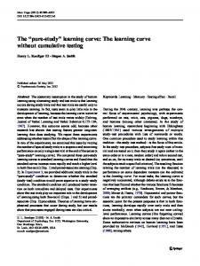
Fig. 1a–d. Indicative color segmentation results for an image of a car. a Original image. b Segmented image (first stage). c Segmented image (final result). d Obtained object contour

As mentioned in Sect. 2, color and motion segmentation results substantially affect the performance of the normalization schemes. The latter is generally true for any contour modeling and curve-matching approach based on natural data. In the present study existing color and motion segmentation algorithms in the literature were tested in order to obtain the best possible object contours from static images and image sequences. In this context, the M-RSST approach yielded adequate results for color objects in high resolution images, while motion segmentation was performed on the basis of 2-D parametric motion models. Some indicative color segmentation results for a still image of a car are illustrated in Fig. 1. Figure 1a depicts the original image, while the results of the first and final steps of the segmentation scheme (M-RSST) are depicted in Fig. 1b and c, respectively. The obtained contour in terms of sample points is depicted in Fig. 1d. The derived object contours are next fed to the proposed orthogonalization scheme. It must be pointed out that the proposed algorithm is employed straightforwardly, in the sense that no human interaction is needed with respect to the particular contour and any parameters are initialized once, when the system is set on-line. Results of the algorithm’s performance on the basis of sample points on the obtained contour are illustrated in Fig. 2. A sample contour consisting of 100 sample points, obtained from color segmentation on a still image containing a fish, is depicted on the upper right-hand side of Fig. 2a. Two other sample curves consisting of 100 points are included in the same figure, which were obtained through direct arbitrary affine transformations of the original sample points. Following the above-described methodology, the sample points of all three curves were subjected to translation, skewing, scaling, rotation, and startingpoint normalization. In this sense, the resulting sample sets are depicted in Fig. 2b–d after translation, skewing/scaling, and rotation/starting-point normalization, respectively. In all cases, the starting point and orientation of the curves are denoted by an arrow. It can be seen that the final sample curves match perfectly when the initial curves are affine transformations of the same sample curve, verifying the results of Sects. 4 and 5. The computational cost of the normalization procedure is negligible: for curves consisting of 100 sample

88

Y. Avrithis et al.: Affine-invariant curve normalization for object shape representation, classification, and retrieval

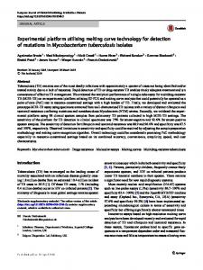
Fig. 2a–d. Intermediate and final results of the proposed orthogonalization scheme on the samples of a fish contour (no resampling scheme was employed). a Original contour and a pair of arbitrary affine transformations. b Curves after translation normalization. c Curves after scaling normalization. d Final curves

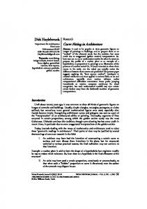
points, the average execution time is of the order of 2 ms using a nonoptimized Matlab implementation on a 266 MHz Pentium II PC. The execution time increases linearly with sample size, as only two of the FFT coefficients are required in the computations. The resulting (orthogonalized) sample sets are identical only when derived from affine transformations of one particular sample curve. In this context, Fig. 3 demonstrates mismatching of orthogonalized curves derived from a particular initial contour of a fish under different (and nonuniform) sampling. In Fig. 3a, the initial sample curve is transformed using a pair of arbitrary affine transformations and the resulting curves are then resampled using nonuniform sampling. The results obtained from the normalization steps are subsequently depicted in Fig. 3b–d. It can be seen that the results are not far from the desired ones, even for significant differences in the sampling process. However, the observed dissimilarities can be annoying when the particular application requires high accuracy in the curve matching. The obtained results can be significantly improved by performing a resampling scheme along with the proposed normalization schemes. Cubic B-splines have been utilized for this purpose, as knot point fitting and reallocation appeared to yield adequate results in terms of uniform sampling (see Sect. 3). Figure 4 illustrates the improvement in matching between orthogonalized curves by performing B-spline modeling and knot point reallocation twice; namely, before translation normalization and before starting-point/rotation rejection. A final resampling step is taken on the basis of the final curves, so as their knot points correspond and the matching technique is enhanced. The plots illustrated in Fig. 4 are directly comparable with that of Fig. 3. When re-

Fig. 3a–d. Results of the proposed orthogonalization scheme on the samples of a fish contour after nonuniform resampling on input curves. a Original contour and arbitrary affine transformations. b,c,d Mismatching of curves after translation, scaling, and rotation normalization, respectively

ferring to orthogonalized curves we will hereon assume that B-spline modeling and knot point reallocation is performed twice, along the lines of the aforementioned methodology. Maybe the most important property of the proposed approach is its ability to align curves that appear to be spatially “similar”. The latter was tested over several object contours belonging to distinct object classes, such as fish, airplanes, cars, glasses, and hammers. Figure 5 illustrates orthogonalization results for three distinct airplanes obtained through color segmentation, and consequently under substantially different sampling. The proposed approach, along with the closed cubic B-spline framework, successfully aligned spatially relative object contours. The orthogonalization results in Fig. 5 should be directly compared to those of Fig. 6, where three sample curves belonging to distinct object classes are employed. It can be seen that, compared to those of Fig. 6d, the final curves of Fig. 5d yield a better resemblance on the basis of almost any matching scheme. The proposed approach yields adequate results even in the presence of significant amount of noise in the sample curves. In order to model noise in object contours due to color/motion segmentation pitfalls, random noise with relatively large variance values was artificially induced into the available object contours. The algorithm’s performance proved to be adequate even in this case, as long as the object contour was not severely deformed. Indicative experimental results are provided in Fig. 7. In Fig. 7a, an object contour corresponding to an airplane along with two noisy counterparts are depicted, one of which is contaminated with twice the amount of noise (in terms of standard deviation) as the other. The respective normalization results are given in Fig. 7b. It must be pointed out here that arti-

Y. Avrithis et al.: Affine-invariant curve normalization for object shape representation, classification, and retrieval

89

Fig. 6a–d. Alignment of orthogonalized contours for substantially different object contours. a Original contours of a hammer, car, and airplane. b,c,d Curves after translation, scaling, and rotation normalization, respectively

Fig. 4a–d. Improvement of orthogonalization results employing B-spline knot modeling and reallocation on the nonuniform sampled curves of Fig. 3. a Original contour and arbitrary affine transformations. b,c,d Curves after translation, scaling, and rotation normalization, respectively

Fig. 7a–d. Orthogonalization results in the presence of random noise in the initial curve samples. a,b Initial and final curves for three instances of the same contour. c,d Initial and final curves for spatially (semantically) relative objects Fig. 5a–d. Immediate alignment of orthogonalization results for semantically similar (spatially similar) object contours. a Original contours for three distinct airplanes. b,c,d Curves after translation, scaling, and rotation normalization, respectively

ficial noise was induced to the nonuniform samples of the initial curves prior to B-spline modeling. As can be seen in Fig. 7b, the “less” noisy instance yields superior matching results than the “more” noisy one. In Fig. 7c and d, relevant results are depicted employing three spatially similar objects (airplanes). As stated in the Introduction, object classification based on contour information has been tackled by several authors, and thus it is not analyzed thoroughly in this paper. However, some indicative classification results have been included in

Fig. 8. Both the prototype contour 1 and the example contour 2 have been subjected to the proposed normalization procedure. Their “normalized” counterparts were compared on the basis of three simple metrics, namely the Euclidean distance of: (a) the respective point sets, (b) the estimated Fourier descriptors, and (c) the modified Fourier descriptors proposed in Rui et al. (1998). As was both intuitively expected and experimentally verified, all three metrics fail for the initial data sets. On the contrary, they prove to be indicative of the normalized curve resemblance (see Fig. 8). Each set of distances was normalized so that 0 and 1 values denote absolute resemblance and no resemblance, respectively. Finally, the proposed algorithm’s performance was successfully tested for content-based retrieval purposes based on

90

Y. Avrithis et al.: Affine-invariant curve normalization for object shape representation, classification, and retrieval

trieval or even video coding, since its computational cost is low. Enhancement and generalization of this normalization procedure is possible in several directions. First, it could be modified to handle sets of connected or unconnected, open or closed curves for the purpose of optical character recognition or indexing of technical line-drawing databases. Normalization of 2-D image data apart from object contours, or even 3-D models and multidimensional data is also desirable, while a very active field of research is normalization with respect to perspective transformation. Such subjects are currently under investigation. Appendix A: Proof of Proposition 1

Fig. 8. Indicative estimated contour distances for classification purposes (FD, Fourier Descriptors; MFD, Modified Fourier Descriptors)

contour similarity on a small database containing 50 still images of 5 visually distinct object classes: namely, airplanes, cars, fish, hammers, and glasses. To obtain best results, particular care was taken so that the main object contours were successfully extracted. In Fig. 9, relevant experimental results are illustrated for an input image containing a airplane. The input image is depicted in Fig. 9a, its extracted contour is shown in Fig. 9b, while the retrieved images are given in descending contour similarity in Fig. 9c. Similar results for an input image containing a car are given in Fig. 10. It must be pointed out for Fig. 9a that by utilizing only the object contour attribute, a fish could yield higher resemblance to an F-15 aircraft than a Stealth aircraft would. For such reasons, the proposed methodology could be employed along with other image attributes such as color and texture information in an integrated content-based retrieval system. It should be noted finally that the proposed technique concentrates only on curve normalization and does not treat the shape retrieval problem by itself; therefore, the results presented in this section can be characterized as indicative. Apart from the normalization scheme, a real-world shape retrieval system would also require a suitable shape-matching algorithm.

7 Conclusions – further work Using the curve normalization procedure presented in this paper it is possible to obtain an affine-invariant curve representation without any actual loss of information on the original curve. The procedure can be applied as a preprocessing step to any shape representation, classification, recognition, or retrieval technique, since it effectively decouples the problem of affine-invariant description from feature extraction and pattern matching. This is verified by employing a number of well-known curve-matching methods in the context of content-based retrieval from image and video databases. In all cases, the proposed normalization is experimentally shown to be considerably robust to shape deformations and noise. Moreover, the technique is very efficient and can be integrated into any real-time system for content-based re-

The restriction that s does not represent a straight-line segment is required so that under any translation, rotation or nonzero scaling transformation, s does not lie on the x or y axis, thus m20 (s) = / 0, m02 (s) = / 0 and all quantities involved in (12)–(15) can be defined. It can be seen that m10 (s1 ) = m01 (s1 ) = 0. This property is also retained for na (s) = s4 , since the remaining normalization steps only involve scaling and rotation. It is also evident that m20 (s2 ) = m02 (s2 ) = m20 (s4 ) = m02 (s4 ) = 1. It is thus observed that 1 m11 (s3 ) = x3 yT3 = (x2 − y2 )(x2 + y2 )T 2 1 (1) = (m20 (s2 ) − m02 (s2 )) = 0 2 so that m11 (s4 ) = m11 (s3 )/(m20 (s3 )m02 (s3 ))1/2 = 0, and therefore na (s) satisfies (17). If angle θ0 = π/4 is substituted by an arbitrary angle θ in (14), then  x2 cos ϑ − y2 sin ϑ s3 = Rϑ s2 = (2) x2 sin ϑ + y2 cos ϑ and (1) is rewritten as m11 (s3 ) = x3 yT3

  = sin ϑ cos ϑ x2 xT2 − y2 yT2   +(cos2 ϑ − sin2 ϑ) x2 yT2   = cos(2ϑ) x2 yT2

(3)

so in order for m11 (s3 ) to be always equal to zero for any initial curve, θ must satisfy cos(2θ) = 0 and therefore take values kπ/2 + π/4, k ∈ Z. Appendix B: Proof of Proposition 2 From (16), na (s) = N(s)(s − µ(s)) = N(s)s1 and na (s ) =  N(s )s1 = N(s )As1 . Since √ s and s are not line segments, det N(s) = σx σy τx τy / 2 = / 0 (and similarly for N(s )), so the two normalization matrices are nonsingular and we can define  q11 q12  −1 Q = N(s )A[N(s)] = (4) q21 q22 so that na (s ) = Qna (s). Now since both na (s) and na (s ) are normalized, we obtain from (19)

Y. Avrithis et al.: Affine-invariant curve normalization for object shape representation, classification, and retrieval

91

Fig. 9a–c. Image retrieval results (query-byexample) based on contour similarity for an input image containing an airplane. a Input image. b Extracted contour. c Retrieved images

Fig. 10a–c. Image retrieval results for an input image containing a car. a Input image. b Extracted contour. c Retrieved images

2 2 m20 (na (s )) = q11 + q12 =1

(38a)

2 2 m02 (na (s )) = q21 + q22 =1

(38b)

m02 (na (s )) = q11 q21 + q12 q22 = 0

(38c)

Thus QQT = QT Q = I2 and Q is an orthogonal matrix, meaning that na (s) and na (s ) differ only in a rotation

transformation (if det Q = 1), plus a possible reflection transformation when det Q = −1. ˜ Now let N(s) be another normalization scheme for s ˜ yielding a normalized curve n˜ a (s) = N(s)s 1 . In this case −1 ˜ = N(s)[N(s)] ˜ na (s), ˜ we can define Q so that n˜ a (s) = Q and since both na (s) and n˜ a (s) are normalized, we can sim˜ is orthogonal. Therefore all possible ilarly conclude that Q normalization schemes based on (17) result in a curve that

92

Y. Avrithis et al.: Affine-invariant curve normalization for object shape representation, classification, and retrieval

is related to the proposed na (s) by a mere rotation (or reflection).

Appendix C: Proof of Proposition 3 If z = Sm (z), then (25) holds and we can substitute a1 = (a1 + 2πm/N ) mod 2π and aN −1 = (aN −1 − 2πm/N ) mod 2π into   N    p(z ) = (a − aN −1 ) mod N/2 (39) 4π 1 Moreover, if N is even, N/2 is integer and we can interchange the integer part · and mod N/2 operators. This gives

   N p(z ) = (a1 − aN −1 ) mod N/2 + m mod N/2 (40) 4π which leads to (28a). Now considering that np (z) is obtained from z through a circular shift of N − p(z), we can use (28a) for z and np (z): p(np (z)) = p(SN −p(z) (z)) = (p(z) + (N − p(z))) mod N/2 = 0 

(41)

p(z ) = (p(z) + m) mod N/2  p(z) + m, 0 ≤ p(z) + m < N/2 = p(z) + m − N/2, N/2 ≤ p(z) + m < N

(42)

into the previous relation, which leads to (28c). Finally, note that if N is not even, interchanging the integer part · and mod N/2 operators in (39) may lead to an error of ±1 sample in the estimation of p(z ) from p(z), possibly causing an additional shift of ±1 sample between np (z) and np (z ). Appendix D: Proof of Proposition 4 If s = Qs and Q is decomposed as in (29), then (30) holds and we can find a relation between the discrete Fourier transforms u = (z) and u = (z ): N −1


zi w−ki = sx ejθ

i=0

 =

N −1


(xi + jλyi )w−ki

i=0

sx e uk ,

λ=1

sx ejθ u∗N −k ,

λ = −1

jθ

then from (33a) it follows that z1 = sx (x + jλy)ej(θ−((λr(z)+θ)modπ)) = sx l(z)(x + jλy)e−jλr(z)  sx l(z)z1 , λ = 1 = sx l(z)z∗1 , λ = −1

(46)

so that x1 = sx l(z)x1 and y1 = λsx l(z)y1 = sy l(z)y1 . Hence x1 and y1 differ from x1 and y1 only in their signs, and calculation of their third-order moments in (32a) gives vx (z1 ) = sx l(z)vx (z1 ) and vy (z 1 ) = sy l(z)vy (z1 ). Subsequent normalization (32b) gives x2 = (sx l(z))2 vx (z1 )x1 = x2 and similarly y2 = y2 , and (33b) follows. Finally, (33c) can be directly verified using (32) and (33a).



and a similar argument for z and np (z ) leads to (28b). Next, consider that np (z) = S−p(z) (z) and np (z ) = S−p(z
) (z ) = Sm−p(z
) (z), so that np (z ) = Sp(z)+m−p(z
) (np (z)). But then we can substitute

uk =

Adding the previous two relations, we get (a1 + aN −1 ) mod 2π = (λ(a1 + aN −1 ) + 2θ) mod 2π, since sx = ±1 and thus (2arg sx ) mod 2π = 0. From the definition (31a) of r(z), (33a) follows immediately.
Now evaluation of z1 from (31b) yields z1 = z e−jr(z ) =
sx (x + jλy)ej(θ−r(z )) . If we define  1, λr(z) + θ ∈ [0, π) l(z) = (45) −1, λr(z) + θ ∈ [π, 2π)

(43)

for k = 0, 1, . . . , N −1, where λ = sx sy = ±1. If we evaluate the phases a = arg u and a = arg u , (43) leads to  a1 + θ + arg sx , λ=1  a1 = −aN −1 + θ + arg sx , λ = −1  aN −1 + θ + arg sx , λ=1 (44) aN −1 = λ = −1 −a1 + θ + arg sx ,

Acknowledgement. This work was partially funded by the National Program “YPER” by the General Secretariat of Research and Development of Greece entitled “Efficient Content-Based Image and Video Query and Retrieval in Multimedia Systems”.

References Arkin EM, Chew LP, Huttenlocher DP, Kedem K, Mitchell JSB (1991) An efficiently computable metric for comparing polygonal shapes. IEEE Trans Pattern Anal Mach Intell 13: 209–216 Avrithis Y, Doulamis N, Doulamis A, Kollias S (1998) Efficient content representation in MPEG video databases. In: Proceedings of the IEEE workshop of Content-Based Access of Image and Video Libraries. Santa Barbara, Calif., 21 June, pp 91–95 Avrithis YS, Doulamis AD, Doulamis ND, Kollias SD (1999) A Stochastic framework for optimal key frame extraction from MPEG video databases. Comput Vis Image Understand 75: 3–24 Avrithis Y, Xirouhakis Y, Kollias S (2000) Affine-invariant curve normalization for shape-based retrieval. In: Proceedings of the International Conference on Pattern Recognition, Barcelona, Spain, 4–7 September, pp 1015–1018 Balslev I (1998) Noise tolerance of moment invariants in pattern recognition. Pattern Recog Lett 19: 1183–1189 Bimbo AD, Pala P (1997) Visual image retrieval by elastic matching of user sketches. IEEE Trans Pattern Anal Mach Intell 19: 121–132 Blum H (1967) A transformation for extracting new descriptors of shape. In: Wathen-Dum W (ed) Models for the perception of speech and visual form. MIT Press, Cambridge, Mass. Chang S-F, Chen W, Meng HJ, Sundaram H, Zhong D (1998) A fully automated content-based video search engine supporting spatiotemporal queries. IEEE Trans Circuits Syst Video Technol 8: 602–615 Cohen FS, Huang Z, Yang Z (1995) Invariant matching and identification of curves using B-splines curve representation. IEEE Trans Image Process 4: 1–10 Doulamis AD, Avrithis YS, Doulamis ND, Kollias SD (1999) Interactive content-based retrieval in video databases using fuzzy classification and relevance feedback. In: Proceedings of the IEEE International Conference on Multimedia Computing and Systems, Florence, Italy, 7–11 June, pp 954–958

Y. Avrithis et al.: Affine-invariant curve normalization for object shape representation, classification, and retrieval

Doulamis ND, Doulamis AD, Avrithis YS, Ntalianis KS, Kollias SD (2000) Efficient summarization of stereoscopic video sequences. IEEE Trans Circuits Syst Video Technol 10: 501–517 Flickner M, Sawhney H, Niblack W, Ashley J, Huang Q, Dom B, Gorkani M, Hafner J, Lee D, Petkovic D, Steele D, Yanker P (1995) Query by image and video content: the QBIC system. IEEE Comput Mag 28: 23–32 Freeman H (1970) Boundary encoding and processing. In: Lipkin BS, Rosenfeld A (eds) Picture processing and psychopictorics. Academic, New York Hamrapur A, Gupta A, Horowitz B, Shu CF, Fuller C, Bach J, Gorkani M, Jain R (1997) Virage video engine. In: SPIE Proceedings on Storage and Retrieval for Video and Image Databases V, San Jose, Calif., February, pp 188–197 Hu MK (1962) Visual pattern recognition by moment invariants. IRE Trans Inf Theory 8: 179–187 Huang Z, Cohen FS (1996) Affine-invariant B-spline moments for curve matching. IEEE Trans Image Process 5: 1473–1480 Ip HS, Shen D (1998) An affine-invariant active contour model (AI-snake) for model-based segmentation. Image Vis Comput 16: 135–146 ISO (1997) Text of ISO/IEC MPEG-7: context and objectives V5. ISO/IEC JTC1/SC29/WG11 N1920, Fribourg, October ISO (1998) Text of ISO/IEC MPEG-4: video verification model V11.0. ISO/IEC JTC1/SC29/WG11 N2172, Tokyo, March Jain AK, Zhong Y, Lakshmanan S (1996) Object matching using deformable templates. IEEE Trans Pattern Anal Mach Intell 18: 267–278 Jiang X, Bunke H, Widmer-Kljajo D (1999) Skew correction of document images by focused nearest-neighbor clustering. In: Proceedings of the Fifth International Conference on Document Analysis and Recognition, Bangalore, India, 20–22 September, pp 629–632 Khotanzad A, Hong YH (1990) Invariant image recognition by Zernike moments. IEEE Trans Pattern Anal Mach Intell 12: 489–497 Lai KK, Chin RT (1995) Deformable contours: modeling and extraction. IEEE Trans Pattern Anal Mach Intell 17: 1084–1090 Ma WY, Manjunath BS (1997) Netra: a toolbox for navigating large image databases. In: Proceedings of the International Conference on Image Processing, Santa Barbara, Calif., 26–29 October, pp 568–571 Marques F, Llorens B, Gasull A (1998) Prediction of image partitions using Fourier descriptors: application to segmentation-based coding schemes. IEEE Trans Pattern Anal Mach Intell 7: 529–542 Mokhtarian F (1995) Silhouette-based isolated object recognition through curvature scale space. IEEE Trans Pattern Anal Mach Intell 17: 539– 544 Odobez JM, Bouthemy P (1997) Separation of moving regions from background in an image sequence acquired with a mobile camera. In: Li HH, Sun S, Derin H (eds) Video data compression for multimedia computing. Kluwer, Boston, pp 283–311 Pavlidis T, Ali F (1975) Computer recognition of handwritten numerals by polygonal approximation. IEEE Trans Syst Man Cybern 6: 610–614 Pentland A, Picard RW, Sclaroff S (1996) Photobook: content-based manipulation of image databases. Int J Comput Vis 18: 233–254 Persoon E, Fu KS (1986) Shape discrimination using Fourier descriptors. IEEE Trans Pattern Anal Mach Intell 8: 388–397 Pratt I (1996) Shape representation using Fourier coefficients of the sinusoidal transform. Technical Report Series UMCS-96-7-1. University of Manchester, U.K. Rivlin E, Weiss I (1997) Deformation invariants in object recognition. Comput Vis Image Understand 65: 95–108 Rothe I, Susse H, Voss K (1996) The method of normalization to determine invariants. IEEE Trans Pattern Anal Mach Intell 18: 366–375

93

Rui Y, Huang TS, Mehrotra S (1997) Content-based image retrieval with relevance feedback in MARS. In: Proceedings of the International Conference on Image Processing, Santa Barbara, Calif., 26–29 October, pp 815–818 Rui Y, She A, Huang TS (1998) A modified Fourier descriptor for shape matching in MARS. In: Chang SK (ed) Image databases and multimedia search. (Series on software engineering and knowledge engineering, vol 8) World Scientific, Singapore, pp 165–180 Salembier P, Pardas M (1994) Hierarchical morphological segmentation for image sequence coding. IEEE Trans Pattern Anal Mach Intell 3: 639–651 Salembier P, Marques F, Pardas M, Morros R, Corset I, Jeannin S, Bouchard L, Meyer F, Marcotequi B (1997) Segmentation-based video coding system allowing the manipulation of objects. IEEE Trans Circuits Syst Video Technol 7: 60–73 Schmid C, Mohr R (1997) Local grayvalue invariants for image retrieval. IEEE Trans Pattern Anal Mach Intell 19: 530–535 Shen D, Ip H (1997) Generalized affine invariant image normalization. IEEE Trans Pattern Anal Mach Intell 19: 431–440 Sikora T (1997) The MPEG-4 video standard verification model. IEEE Trans Circuits Syst Video Technol 7: 19–31 Smith JR, Chang SF (1996) VisualSEEk: a fully automated content-based image query system. In: Proceedings of the ACM Multimedia Conference, Boston, Mass., 18–22 November, pp 87–98 Swanson MD, Tewfik AH (1997) Affine-invariant multiresolution image retrieval using B-splines. In: Proceedings of the International Conference on Image Processing, Santa Barbara, Calif., 26–29 October, pp 831– 834 Taubin G, Cooper D (1992) Object recognition based on moment (or algebraic) invariants. In: Mundy JL, Zisserman A (eds) Geometric invariance in computer vision. MIT Press, Cambridge, Mass., pp 375–397 Tekalp M (1995) Digital video processing. Prentice Hall, Upper Saddle River, N.J. Torres L, Kunt M (1996) Video coding: the second generation approach. Kluwer, Boston Tsang PWM (1997) A genetic algorithm for affine invariant recognition of object shapes from broken boundaries. Pattern Recog Lett 18: 631–639 Wang J, Cohen FS (1994) Part II: 3-D object recognition and shape estimation from image contours using B-splines, shape invariant matching, and neural network. IEEE Trans Pattern Anal Mach Intell 16(1): 13–23 Wang J, Yang W-J, Acharya R (1998) Efficient access to and retrieval from a shape image database. In: Proceedings of the IEEE workshop of Content-Based Access of Image and Video Libraries. Santa Barbara, Calif., 21 June, pp 63–66 Watt A, Watt M (1992) Advanced animation and rendering techniques. ACM Press, New York Xirouhakis Y, Avrithis Y, Kollias S (1998) Image retrieval and classification using affine invariant B-spline representation and neural networks. In: Proceedings of the IEE Colloquium on Neural Nets and Multimedia, London, 22 October, pp 4/1–4/4 Xirouhakis Y, Mathioudakis V, Delopoulos A (1999a) An efficient algorithm for mobile object localization in video sequences. In: Proceedings of the Visual, Modeling and Visualization Workshop, Erlangen, Germany, 17–19 November, pp 117–124 Xirouhakis Y, Tirakis A, Delopoulos A (1999b) An efficient graph representation for image retrieval based on color composition. In: Mastorakis N (ed) Advances in intelligent systems and computer science. World Scientific and Engineering Society, New York, pp 336–341 Yang Z, Cohen FS (1999) Image registration and object recognition using affine invariants and convex hulls. IEEE Trans Pattern Anal Mach Intell 8: 934–946

94

Y. Avrithis et al.: Affine-invariant curve normalization for object shape representation, classification, and retrieval

Yannis S. Avrithis was born in Athens, Greece, in 1970. He received the Diploma degree in Electrical and Computer Engineering from the National Technical University of Athens (NTUA) in 1993, the M.Sc. degree in Electrical and Electronic Engineering (Communications and Signal Processing) from the Imperial College of Science, Technology and Medicine, London, U.K., in 1994, and the Ph.D. degree in Electrical and Computer Engineering from NTUA in 2001. He is currently a senior researcher at the Image, Video and Multimedia Systems Laboratory of NTUA. His research interests include digital image and video processing, image segmentation, affine-invariant image representation, content-based indexing and retrieval, and video summarization. He has published 7 articles in international journals and books, and 17 in proceedings of international conferences. Yiannis S. Xirouhakis was born in Athens, Greece, in 1975. He received his degree in Electrical and Computer Engineering from the National Technical University of Athens (NTUA) in 1997. Currently he is a Ph.D. candidate in the Image, Video and Multimedia Systems Laboratory of the Electrical and Computer Engineering Department of NTUA. His main area of research includes computer vision and video understanding; more precisely, 3-D motion and structure estimation, object recognition, and video indexing. As a student he received several national awards in Greece in mathematics and physics. He has published 25 articles in international journals and conferences in his area of research.

Stefanos D. Kollias was born in Athens, Greece, in 1956. He received the Diploma degree in Electrical Engineering from the National Technical University of Athens (NTUA) in 1979, the M.Sc degree in Communication Engineering from the University of Manchester (UMIST), U.K., in 1980, and the Ph.D degree in Signal Processing from the Computer Science Division of NTUA in 1984. In 1982 he received a ComSoc Scholarship from the IEEE Communications Society. Since 1986 he has been with the NTUA where he is currently a Professor. From 1987 to 1988, he was a Visiting Research Scientist in the Department of Electrical Engineering and the Center for Telecommunications Research, Columbia University, New York, U.S.A. His current research interests include image processing and analysis, neural networks, image and video coding, and multimedia systems. He is the author of more than 140 articles in the aforementioned area.