exactly 1 or 2 out of 5 possibilities are true seems to require enumerating all .... representation and query answering on every possible world ..... Writing B = âm.
Aggregate Query Answering on Possibilistic Data with Cardinality Constraints Graham Cormode
Divesh Srivastava
AT&T Labs – Research {graham, divesh}@research.att.com
Abstract— Uncertainties in data arise for a number of reasons: when the data set is incomplete, contains conflicting information or has been deliberately perturbed or coarsened to remove sensitive details. An important case which arises in many real applications is when the data describes a set of possibilities, but with cardinality constraints. These constraints represent correlations between tuples encoding, e.g. that at most two possible records are correct, or that there is an (unknown) one-to-one mapping between a set of tuples and attribute values. Although there has been much effort to handle uncertain data, current systems are not equipped to handle such correlations, beyond simple mutual exclusion and co-existence constraints. Vitally, they have little support for efficiently handling aggregate queries on such data. In this paper, we aim to address some of these deficiencies, by introducing LICM (Linear Integer Constraint Model), which can succinctly represent many types of tuple correlations, particularly a class of cardinality constraints. We motivate and explain the model with examples from data cleaning and masking sensitive data, to show that it enables modeling and querying such data, which was not previously possible. We develop an efficient strategy to answer conjunctive and aggregate queries on possibilistic data by describing how to implement relational operators over data in the model. LICM compactly integrates the encoding of correlations, query answering and lineage recording. In combination with off-the-shelf linear integer programming solvers, our approach provides exact bounds for aggregate queries. Our prototype implementation demonstrates that query answering with LICM can be effective and scalable.
I. I NTRODUCTION Lately, the data management community has invested much effort in dealing with non-exact data, which may be incomplete, perturbed or masked such that conventional database systems fail to manage them effectively [1], [2], [3], [4]. Such uncertain data arises in many domains, including data integration, data cleaning, anonymization and others, all of which naturally result in large amounts of non-exact data. Many approaches have been proposed to manage uncertainty in databases. Among these, models which can handle tuple-level correlations among uncertain tuples [1], [3], [5], [6] are particularly important, due to the dependencies between tuples that often occur in real data. For instance, records generated by a sensor network naturally have correlations in space and time. However, the correlations which we call cardinality constraints, are prevalent in real applications but are rarely explicitly handled in prior work. Consequently, existing systems do not effectively answer queries with such constraints. In this paper we focus on modeling and query an-
Entong Shen
Ting Yu
North Carolina State University {eshen,tyu}@ncsu.edu
swering on this type of correlated data. We first introduce and motivate cardinality constraints in two different applications: Example 1: Suppose that in a data cleaning and integration scenario we have five different records of the address of the same customer, arising from different sources. It is known that at least one and at most two out of the five records are correct (home and office addresses). Without further information or conflict resolution rules, it is reasonable to retain all five records in an uncertain database to reason over. Then all analysis must respect the constraint on the cardinality expressed above. For example, suppose that the data is to be used to plan an advertising campaign. An example query to ask is ‘At most how many regions are there in the United States having more than a thousand of our customers?’. Answering this query requires us to place a (tight) upper bound on the answer, based on the cardinality constraints in the data. Example 2: Cardinality constraints also arise in data which has had its precision reduced to provide privacy. For instance, the sensitive attributes (e.g. disease) of a group of individuals may be permuted such that there exists a bijective mapping between the group of individuals and the group of attributes. Suppose that {Alice, Bob, Carol} is associated with {flu, cancer, heart disease}. The cardinality constraint encoded is twofold: each entity has exactly one attribute and each attribute is associated with exactly one entity. In this example a researcher would like to know ‘At least how many male patients are there who do not have cancer?’. These sorts of cardinality constraints over possibilistic data are quite natural and common. However, no existing models provide ways to directly model them, instead requiring awkward formulations or exhaustive enumeration. In possibilistic data with cardinality constraints, we typically want to answer aggregate queries (as in our motivating examples), about sums or counts of values in the data, or conditions on cardinalities like having COUNT > d. But existing work on uncertain data provides weak support, if any, for aggregation. While correlations between tuples are handled by many working models [3], [1], [5], [4], these do not adequately handle cardinality constraints. Their focus has been on more logical constraints (implications, mutual exclusions or co-occurrences) which, while expressive, do not naturally capture cardinalities. In this work we introduce a new model for representing and querying data with cardinality constraints, the Linear Integer Constraint Model (LICM) and show that it succinctly repre-
sents a variety of data with cardinality constraints (and other simpler correlations as well). LICM takes advantage of integer valued variables and linear constraints on those variables. As for query processing, rather than querying each possible world encoded by LICM, we instantiate the behavior of relational operators so that query processing can take place within the LICM framework. In line with the motivating examples, we focus on providing upper and lower bounds on aggregate query answers: without further semantics of the uncertain data, we must consider all consistent possible worlds, and hence seek to bound these answers. The exact upper and lower bounds provide us two extreme points on the spectrum of the query answers, which can be further used for best/worst case analysis to answer queries like those in Examples 1 and 2. The bounds are implied by a collection of linear integer constraints which encode the lineage of tuples. This problem naturally forms a binary integer programming (BIP) problem, which we can solve using off-the-shelf linear programming solvers to obtain the exact minimum and maximum values of aggregate queries. Modern solvers are able to handle large optimization problems very efficiently [7]. They can exploit the structure within the BIP instances generated, and solve efficiently even for 105 to 106 variables and constraints, as we confirm in experiments. To make the presentation more concrete, we provide examples of the LICM approach in the context of imprecise transaction data, in the form of set-valued data with cardinality constraints. In set-valued data, each logical entity is associated with a set of values. Examples of such data include retail transaction information, health care records and search logs. Contributions. We summarize our contributions as follows: We propose LICM, a novel working model for uncertain data that can succinctly represent data with complex correlations among tuples including cardinality constraints. We show that it is complete for finite sets of possible worlds and it is closed under conjunctive relational algebra by carefully devising the set of linear constraints which correctly encode the semantics of each operator. This implies a systematic method for query answering. • LICM compactly integrates encoding of correlations, query processing and data lineage such that it does not necessitate explicit lineage representation or materialization of possible tuples, as required in prior work. LICM is able to answer queries in a purely relational way which does not introduce new operators and thus can benefit from existing query optimization techniques. (Section III and IV) • Using LICM, it is possible to obtain not only the expected value of an aggregate query, but also the upper and lower bounds which are useful for best/worst case analysis by naturally formulating the LICM representation of the query answer as a binary integer programming problem. The bounds of aggregate query answers can be found readily using off-the-shelf integer program solvers. (Section IV-D) • We conduct extensive experiments to evaluate the effectiveness and efficiency of LICM approach and compare it to the Monte-Carlo sampling approach. The experimental •
results show that LICM combined with linear programming solvers can efficiently and accurately compute bounds on aggregate query answers over uncertain data. (Section V) II. R ELATED W ORK In this section, we show that while the various models introduced have many strengths, they cannot work with cardinality constraints well. Specifically, we note that in all prior work, either the models do not naturally represent these constraints (making it impossible or very expensive to represent the input), or they do not support efficient answering of aggregate queries that we focus on (they either omit aggregation operations, or require exploration of exponentially many possibilities). Consequently, we conclude that new approaches are needed for the problems described in the introduction. ULDBS, WSDs and U-relations. ULDBs [3] are a representation system that deal with both uncertainty and lineage. The underlying model uses ‘x-tuples’ plus three-valued logic to represent the uncertain data. The model itself is not complete. But integrated with lineage information, it facilitates the correlation and coordination of uncertainty in query results with uncertainty in the input data. Antova et al. [2] introduce worldset decompositions (WSDs) which lists several components whose Cartesian product reconstitutes the full relation. Urelations extend WSDs by introducing an extra column D which encodes the conditions for each tuple to occur, based on variables, and a table containing possible assignments of variables [1]. E.g., condition x → 1, y → 2 indicates that the tuple exists only when the variable x is set to 1 and y to 2. Ranging over all assignments to variables provides the set of possible worlds. This is effective in encoding correlations such as alternatives, but does not naturally allow cardinality constraints. In Example 1, representing the constraint that exactly 1 or 2 out of 5 possibilities are true seems to require enumerating all possibilities. Similarly, consider the uncertain transaction data in Figure 2(a), where some items in the transaction are only known approximately, according to the hierarchy in Figure 2(b): the “alcohol” in Transaction T1 could be any non-empty subset of {Beer, Wine, Liquor}. Representing this knowledge in Urelations is cumbersome: Figure 1 illustrates one possible encoding which enumerates all the non-empty subsets. Even if we can represent our data in this form, there has been no work on answering aggregate queries over U-relations.1 Hence, U-relations and its antecedents do not apply to problems involving cardinality constraints. Probabilistic Graphical Models. Probabilistic graphical models [6], [5] represent a popular class of models used to handle correlations in probabilistic data. The probabilistic and/xor tree model [5] generalizes the Block-Independent Disjoint model by considering combinations of two types of correlations (co-existence and mutual exclusion) between tuples or attributes. Again, we consider the constraint from Example 1 1 Where aggregates have been considered, they required enumeration of exponentially many possible worlds, or give bounds only on expected values.
TID T1 T1 T1 T1 T1 T1 Fig. 1.
LNodeID Beer Wine Liquor Beer Wine Beer
D TID LNodeID x→1 T1 Liquor x→2 T1 Wine x→3 T1 Liquor x→4 T1 Beer x→4 T1 Wine x→5 T1 Liquor x 7→ {1, 2, 3, 4, 5, 6, 7}
D x→5 x→6 x→6 x→7 x→7 x→7
U-relation encoding of first alcohol item in Fig 2(a)
that exactly 1 or 2 out of 5 tuples exist. Certainly this can be represented as the mutual exclusivity of the 15 possibilities (10 worlds of two items, and 5 of one), but this enumeration is unacceptable when the number of possible tuples in a block is large (e.g., up to 20) because of the exponential number of possibilities encoded. Other models use Bayesian networks to capture more general correlations [6]. These models rely on factored representations to allow computation of the joint distribution of all possible tuples as a product of distributions over pairwise (or small groups of) correlated tuples. Across all methods based on probabilistic representations of data, some fundamental roadblocks arise to representing data with cardinality constraints. In our motivating examples, the input does not provide probabilities of different events, only a description of the possibilities, and we require reasoning over all of these to correctly answer aggregate queries. That is, there is no meaningful way to assign probabilities to the different possibilities. It is tempting to make some uniformity assumptions (treat all outcomes as equally likely), but this gives a false semantics which is not consistent with the original description of the data. Query answering over probabilistic data, when it has considered aggregate queries, has tended to stick to simple expected values or approximations of the distribution of answers, which are necessarily vague about extremal values [8]. Moreover, they do not offer solutions which do not require exponential enumeration of all possibilities. Other systems support efficient implementations of Monte Carlo methods [9], [12], but empirically we show that such sampling does not explore the full range of possibilities. Thus, these approaches do not provide correct answers for queries such as those described in Examples 1 and 2. C-tables. The c-tables model [10] and its generalizations form a very powerful collection of models. Indeed, our proposed model (as well as U-relations, ULDBs, etc.) can be seen as instances of the c-tables framework with a restricted type of constraints. Previously, there has been little effort to actually implement such powerful models, due to the difficulties in supporting efficient query processing, particularly for the aggregates we focus on. The strength of LICM lies not only in its representation but more importantly the ability to actually answer a wide range of complex queries. Constraint-based Methods. Many papers have used constraints to help model correlations in data, and search for satisfying solutions, which is broadly similar to our approach. The areas of constraint programming and constraint networks [11] consider ways to encode and solve problems with constraints.
Our work adds to this area: to the best of our knowledge, there has been no work which encodes the cardinality constraints of the form we consider here and discusses how to apply query operators to manipulate the representation. Recent work in parallel to this [12] discusses sampling only those possible worlds which satisfy some global aggregate constraints. While ostensibly similar, the problem differs from ours since uncertainty is only over tuple values, and techniques provide a sampling mechanism, not a data model. Summary of Prior Works. Our survey encompassed many more works than there is room to discuss in detail; instead, we have tried to highlight representative examples and expand on the common features present. Overall, while there are many prior efforts relating to various aspects of our work, such as encoding uncertainties, or reasoning via constraints, we did not observe any prior work which is able to capture exactly the space of possible worlds and efficient solutions of LICM for problems involving cardinality constraints. Some models are (much) more general, such as c-tables, but these then suffer since it is unknown how to efficiently answer queries: we deliberately ensure that the model is limited to linear constraints, since these are expressive while producing an optimization problem which is efficiently solvable. III. L INEAR I NTEGER C ONSTRAINT M ODEL We adopt a common interpretation of an uncertain database as a finite set of deterministic database instances D = {D1 , D2 , . . . , D|D| }, which we call possible worlds. Each world is a distinct subset of the tuples present in D. Note that explicit representation and query answering on every possible world is usually not feasible because the number of possible worlds is exponential in the number of tuples in the database. We seek more efficient ways to represent and query the data. As discussed in Section I, cardinality constraints occur naturally in many application domains. Definition 1 (Cardinality constraint): Given a set S of possible tuples, let S˜ ⊂ S be a set of tuples in a possible world. ˜ ≤ Z2 , where Cardinality constraints are of the form Z1 ≤ |S| Z1 , Z2 are integers. Example 3 (Permutation Constraints): A constraint on a collection of tuples that requires them to have a bijective mapping to an equal-sized collection of values (permutation constraints) can be seen as a special case of cardinality constraints. Recall Example 2 which had such a constraint. Let T ID = {tid1 ,tid2 , . . . ,tidn } be a set of tuple IDs which has one-to-one mapping to a set of possible values V = {v1 , v2 , . . . , vn }. We have the following cardinality constraints: For each i, among Si = {(tidi , v1 ), (tidi , v2 ), . . . , (tidi , vn )}, only one tuple exists (in any possible world); for each j, among S j = {(tid1 , v j ), (tid2 , v j ), . . . , (tidn , v j )}, only one tuple exists. Definition 2 (LICM relation): An LICM relation R is a collection of tuples {t1 ,t2 , . . . ,tn } of schema {A1 , . . . , Ak , Ext}, where Ai , i = {1, . . . , k}, are attributes over finite domains and Ext is a special attribute indicating the existence of each tuple. For each tuple t ∈ R, the Ext attribute can be either ‘1’ which confirms the occurrence of t, or a binary variable bi ∈ {0, 1}
TID T1 T2 T3 T4 T5 T6
Items Purchased {Alcohol, Shampoo} {Alcohol, Shampoo} {Liquor, Health Care} {Liquor, Health Care} {Shampoo} {Shampoo}
All Alcohol
Beer Wine Liquor
(a) Uncertain transaction data
Health Care
Diapers Pregnancy test Shampoo
(b) An example generalization hierarchy for items Fig. 2.
TID T1 T1 T1 T1
ItemName Beer Wine Liquor Shampoo b1 + b2 + b3 ≥ 1
Ext b1 b2 b3 1
(c) LICM encoding of T1 in Fig. 2(a)
Example data set and different encodings of generalized data
which indicates t is a maybe-tuple. Definition 3 (LICM database): An LICM database D is a tuple (R, C), where R is a set of LICM relations and C is a set of linear constraints on binary variables that may appear in the LICM relations in R. Let B = {b1 , b2 , . . . , b|B| } be the set of all binary variables appearing in D. A linear constraint Ci : fi (B) θ Z is a linear function fi with respect to B ⊆ B, an operator θ ∈ {=, ≥, ≤} and an integer Z. Example 4: Figure 2(c) shows an LICM database for the first transaction in Figure 2(a) with the generalization hierarchy of Figure 2(b). The uncertain transaction data set can be stored in a table T RANS I TEM(TID, ItemName, Ext). The first three tuples are maybe-tuples subject to the constraint below the tuples, ensuring that at least one of them is present. The last tuple (T1 , Shampoo) exists in every possible world. We next define the semantics of an LICM database, i.e., the set of possible worlds defined by D. Given an LICM database D = (R, C), a possible world is obtained when a value of 0 or 1 is assigned to each of the binary variables in B. An assignment A is valid if it satisfies all the linear constraints in C. Given a valid assignment, we eliminate all tuples t in R with t.Ext = 0. An instantiation of D is given by the remaining tuples A(D) = {t(a1 , a2 , . . . , ak ) | t.Ext = 1,t ∈ R, R ∈ R} Each instantiation represents a possible input database that is consistent with the description provided by D. Thus, an LICM database D defines the set of databases (the possible worlds) that are instantiated by all the valid assignments. The introduction of variables is one of the major techniques to represent uncertain information in a database, such as c-tables and U-relations. In the original c-tables approach, variables can be associated with both tuples and attributes, and arbitrary constraints can apply to variables, making it very powerful. Hence, it is challenging to maintain data in the full model, and to evaluate queries. Although LICM only allows linear constraints and association of binary variables with tuples, it does not affect its expressiveness: any finite set of database instances can be described by an LICM database. Theorem 1 (Completeness): LICM is complete for uncertain databases. That is, given any finite set of database instances D, there exists an LICM database D that defines D. Proof: Let D = {D1 , D2 , . . . , Dn } be a finite set of database instances. Let T denote all the tuples in D. Then every database instance consists of a collection T ⊆ T of tuples. Suppose each tuple ti ∈ T is associated with a binary variable bi indicating the tuple’s existence. Then any finite set
of possible worlds can be represented in disjunctive normal form (DNF) over the binary variables. In the DNF representation each disjunctive component represents a database instance D j by conjoining all the binary variables in either positive form bi or negation form ¬bi , depending on the existence (or non-existence) of ti in D j . Each assignment of truth values to binary variables for which the DNF form evaluates to true corresponds to one of the possible worlds. We convert the DNF to conjunctive normal form (CNF) using the standard method. Each conjunctive component must be true. Since for each component the binary variables are in disjunctive form, we can add all bi of positive form and all (1 − bi ) for bi in negation form and let the sum ≥ 1. Writing linear expressions in this way for all conjunctive components encodes all the possible worlds exactly. Succinctness. Given a set S of possible uncertain tuples, LICM represents cardinality constraints over S succinctly using |S| tuples and corresponding cardinality constraints. Each maybetuple is associated with a binary variable, and the linear constraints are written as cardinality constraints on the sum of all those binary variables. The compactness of LICM comes from the expressive power of linear constraints over binary variables and a natural match between LICM and cardinality constraints. In Figure 2(c), LICM concisely represents the same semantics as in Figure 1. Other Correlations. The linear constraints over binary variables in LICM can naturally represent not only cardinality constraints but also other common correlations. Example 5: Suppose two uncertain tuples t1 and t2 are associated with binary existence variables b1 and b2 respectively. Then linear constraints can easily capture the following correlations: Mutual exclusion: b1 + b2 = 1; Co-existence: b1 − b2 = 0; Material implication (t1 → t2 ): b1 − b2 ≤ 0 In fact, linear constraints over binary variables can represent arbitrary correlations between tuples, as any correlations describe a set of possible worlds and can be encoded via the method in Theorem 1. For disjunctive constraints, LICM may need to perform the costly DNF to CNF conversion. But, as shown above, LICM represents common correlations including cardinality constraints directly and compactly. IV. Q UERY A NSWERING WITH LICM In this section we describe how conjunctive and aggregate queries can be processed in the LICM framework by redefining the behaviors of relational operators. Since an LICM database D describes a set of database instances D = {D1 , D2 , . . . , Dn },
TID T1 T1 T2
ItemName wine liquor beer b1 + b2 ≥ 1
Ext b1 b2 1
TID T1 T2
ItemName wine beer (b) R2
Ext b3 b4
(a) R1
TID T1 T2
ItemName wine beer Fig. 3.
Ext b5 b4
Constraints b1 + b2 ≥ 1, b5 ≤ b1 , b5 ≥ b1 + b3 − 1, b5 ≤ b3 ,
(c) R1 ∩ R2
Algorithm 1 Projection πT ID (R) 1: R˜ ← 0; / C˜ ← C; 2: for all Ti : (Ti , Itemi , Exti ) ∈ R do 3: if ∃(T ID, Item, Ext) ∈ R|(T ID = Ti ) ∧ (Ext = 1) then 4: R˜ ← R˜ ∪ {(T IDi , 1)} 5: else 6: R˜ ← R˜ ∪ {(Ti , b)} for new variable b 7: T ← {(T ID j , b j )|T ID j = Ti , (T ID j , Item j , b j ) ∈ R} 8: ∀t j = (T ID j , b j ) ∈ T : C˜ ← C˜ ∪ {b ≥ b j } 9: C˜ ← C˜ ∪ {b ≤ ∑t j ∈T b j }
Query answering example in LICM
Algorithm 2 Intersection R1 ∩ R2 the semantics of a query Q(D) is to evaluate Q(Di ) for each instance Di . As in [10], our approach is to translate Q to Q0 on the data representation, so that the evaluation of Q0 encodes the answers to Q(Di ), i = 1 . . . n. This is much more efficient than explicitly evaluating the query on each Di separately. A. Overview Example 6: Figure 3 gives an example of how relational algebra operators can be applied to LICM representations, and obtain results which are also in LICM form. Given two LICM databases in Figure 3(a) and Figure 3(b), to process the intersection operator in LICM, we create a new variable b5 and link it to its lineage variables b1 and b3 by a set of new constraints shown in Figure 3(c). The tuple (T1 , wine) is in R1 ∩ R2 (i.e., b5 = 1) if and only if b1 = 1 and b3 = 1. This can be represented by a set of linear constraints: b5 ≤ b1 , b5 ≤ b3 and b5 ≥ b1 + b3 − 1. If either b1 or b3 is 0, b5 must be 0 to satisfy this set of constraints. The way LICM processes queries has advantages over existing models. First, the linear constraints over binary variables integrate representation, query answering and data lineage as a whole. Data lineage is recorded implicitly in the constraints and can be traced when necessary. Second, LICM does not require materializing the possibilities of tuples throughout the entire process of query evaluation. In contrast, ULDB requires traditional query evaluation over all the alternatives of the base x-relations, and the poss operator in U-relations generates the set of all possible tuples [1], [3]. Finally, LICM does not require a new approach to query optimization, since it does not introduce new operators. As can be seen from the above example, the biggest challenge is how we can reason with linear constraints in a systematic and compact way, i.e., how to devise the set of variables and constraints which correctly encode the semantics of an operator. Now we give the details of the algorithms. B. Translation of Conjunctive Operators Selection σ . The behavior of the selection operator σ in LICM framework is natural: given an LICM relation R(A, Ext) with constraint set C and a selection predicate σAθ d , the output LICM relation contains all tuples which satisfy the predicate, along with constraint set C. The constraints are kept unchanged. Some constraints may become irrelevant after selection; these can be dropped, or allowed to remain:
1: R˜ ← 0; / C˜ ← C1 ∪C2 2: for all ti = (T IDi , Itemi , Exti ) ∈ R1 do 3: if ∃t j ∈ R2 : T IDi = T ID j ∧ Itemi = Item j then 4: if (Exti = Ext j ) ∨ (Ext j = 1) then 5: R˜ ← R˜ ∪ {ti } 6: else if Exti = 1 then 7: R˜ ← R˜ ∪ {t j } 8: else 9: R˜ ← R˜ ∪ {(T IDi , Itemi , b)} for new variable b 10: C˜ ← C˜ ∪ {b ≤ bi , b ≤ b j , b ≥ bi + b j − 1}
the solver will eliminate them later. Note that selection and projection (introduced below) operators in LICM can only be posed over the normal attributes, i.e., they cannot explicitly reference the special Ext attribute. Projection π. The projection operator in relational algebra enforces set semantics instead of the bag semantics in SQL. So duplicate tuples (regardless of Ext attribute) should not appear in the resulting relation. Without loss of generality, consider an LICM relation R(TID, ItemName, Ext) with constraint set C. Note that the special attribute Ext is always ˜ For ˜ C). present in an LICM relation. Let D˜ = πT ID (D) = (R, each distinct T ID, if some instance is certain to exist, then a ˜ else a maybe-tuple is added whose certain tuple is added to R, presence depends on the existence of any previous tuple with a matching T ID. Algorithm 1 formally defines the behavior of π under LICM. We illustrate the algorithm with an example: Example 7: Let D be the LICM relation in Figure 4(b). To build πT ID (D), observe that T2 will certainly appear in πT ID (R) because of tuple (T2 ,Wine, 1). T1 should be present if any of b1 , b2 and b3 is true. We first associate T1 with a new binary variable b8 and put (T1 , b8 ) in πT ID (R). New constraints b8 ≥ b1 b8 ≥ b2 b8 ≥ b3 b8 ≤ b1 + b2 + b3 are added to πT ID (C) to encode these semantics. A similar process can apply to T3 , but an optimization is to observe that T3 is unique in D, so R˜ can contain (T3 , b7 ). The resulting table has constraints as defined above and πT ID (R) = {(T1 , b8 ), (T2 , 1), (T3 , b7 )}. Intersection ∩. Given two LICM databases D1 = (R1 ,C1 ) and D2 = (R2 ,C2 ) with schema R(TID, ItemName, Ext), the ˜ is defined in Algorithm 2. ˜ C) intersection D = D1 ∩ D2 = (R, The logic is that a tuple exists in the intersection only if it exists in both input relations. The existence of the new tuple is then derived from the existence of the tuples from each input
Count (*)
Algorithm 3 Product R1 × R2
R '' Cnt ! 2 TID ,COUNT ( ItemName ) !Cnt
R' ItemName "! Shampoo! or !Diaper ! or !Pregnancytest !
R (TID, ItemName) (a) Example query tree Fig. 4.
TID T1 T1 T1 T2 T2 T3
ItemName Pregnancy test Diapers Shampoo Wine Shampoo Pregnancy test
Ext b1 b2 b3 1 b6 b7
(b) Example LICM relation Query answering in LICM
relation. Note that new variables and constraints are created when ti and t j are two maybe-tuples in R1 and R2 and their normal attributes match exactly (they need not match on Ext). The rules to handle Cartesian product (Algorithm 3) are very similar to those of Intersection, as the combination of two maybe-tuples exists in the resulting relation if and only if their binary variables will both be assigned 1. Since Join can be decomposed to a Cartesian product, a selection and a projection, we do not explicitly define a join algorithm: an efficient join operator is built by combining these definitions. A salient feature of query answering with LICM is that by carefully devising a set of linear constraints, each relational operator is processed in a deterministic way, i.e., given an assignment to the variables in the input tables to an operator, there exists only one correct assignment of the variables in the output tuples which satisfy that set of constraints. The correctness of the above algorithms can be easily verified by checking the truth table of each operator. Compared to other uncertain data models, query processing in LICM is much more self-contained and direct. It does not require a rewrite of the original query Q to incorporate new operators like ‘merge’ in the U-relations model [1]. Nor does it need to express and extract lineage information explicitly like in ULDBs [3]— lineage is implicitly encoded in LICM through addition of new variables and constraints. Moreover, since we only redefine the behaviors of operators rather than rewriting the query, the same space of query plans exists as in the traditional relational case (e.g. selections can be pushed down). Since the LICM operators are deterministic, the answers from equivalent query trees will be equivalent even though the sets of variables and representations of constraints may differ. C. COUNT and SUM Operators COUNT and SUM are not core relational algebra operators, but queries involving these operators are extremely common and useful in practice, and hence are central to our efforts. According to their positions in the query tree, aggregate operators may be handled in the following cases: Aggregation at the top. If a COUNT operator appears at the top of the query tree, the count is exactly the sum of all Ext values in the final relation. For example, for the LICM database described in Figure 3(a), a query asks for the number of transactions in which the ItemName attribute is ‘beer’ or
1: R˜ ← 0; / C˜ ← C1 ∪C2 2: for all ti = (T IDi , Itemi , Exti ) ∈ R1 , 3: 4: 5: 6: 7: 8: 9: 10: 11:
t j = (T ID j , Item j , Ext j ) ∈ R2 do if Exti = Ext j then R˜ ← R˜ ∪ {(T IDi , Itemi , T ID j , Item j , Exti )} else if Exti = 1 then R˜ ← R˜ ∪ {(T IDi , Itemi , T ID j , Item j , b j )} else if Ext j = 1 then R˜ ← R˜ ∪ {(T IDi , Itemi , T ID j , Item j , bi )} else R˜ ← R˜ ∪ {(T IDi , Itemi , T ID j , Item j , b)} for new b C˜ ← C˜ ∪ {b ≤ bi , b ≤ b j , b ≥ bi + b j − 1}
Algorithm 4 Intermediate COUNT operator 1: 2: 3: 4: 5: 6: 7: 8: 9: 10: 11: 12: 13: 14: 15:
R˜ ← 0; / C˜ ← C Case 1: COUNT ≤ d if m + n ≤ d then R˜ ← (T, 1) else if n ≤ d then R˜ ← (T, b) for new variable b C˜ ← C˜ ∪ {d − n + 1 ≤ (d − n + 1)b + ∑m i=1 bi } C˜ ← C˜ ∪ {m ≥ (m − d + n)b + ∑m b } i i=1 Case 2: COUNT ≥ d if n ≥ d then R˜ ← (T, 1) else if m + n ≥ d then R˜ ← (T, b) for new variable b C˜ ← C˜ ∪ {(d − n)b ≤ ∑m i=1 bi } C˜ ← C˜ ∪ {d − n − 1 + (m − d + n + 1)b ≥ ∑m i=1 bi }
‘wine’. The COUNT operator is applied in the end after the desired tuples have been selected. Then it is straightforward to obtain an expression for the total count as b1 + 1. Similarly, when SUM is applied over a constant numeric attribute (such as the sum of prices of a subset of items), the result is exactly the sum of each value multiplied by the corresponding Ext value. Other aggregates, such as MIN and MAX can also be handled in a similar way to SUM and COUNT, using case based reasoning to encode their effect in LICM. To focus the discussion, for the remainder of the paper we study the more common case of COUNT. COUNT in the middle. In more complex queries the COUNT operator may also appear in the middle of the query tree. In this case, it is usually associated with a selection immediately above it. In order to more easily represent the resulting relation in LICM, we handle count and selection together and consider a count predicate COUNT θ d. To better illustrate how the count predicate is handled in LICM, we provide an example. Example 8: Consider the query “Count how many transactions include ≥ 2 ‘Health Care’ items” on the dataset shown in Figure 4(b) (the constraint set is not shown). The corresponding query tree, in Figure 4(a), is evaluated bottom-up. Tuple (T2 ,Wine, 1) is dropped by the first selection operator. Considering the count and selection on the count together, T2 cannot appear in R00 because only one tuple involving T2 exists in R0 . The same logic excludes T3 . Tuple T1 in R00 is uncertain, depending on b1 , b2 and b3 . Hence a new binary variable b8
is created and (T1 , b8 ) is put in R00 , while constraints b1 + b2 + b3 ≥ 2b8
b1 + b2 + b3 − 2b8 ≤ 1
encode the desired semantics that b1 + b2 + b3 ≤ 1 ⇐⇒ b8 = 0 b1 + b2 + b3 ≥ 2 ⇐⇒ b8 = 1 The count predicate operator semantics are defined formally in Algorithm 4, and its correctness is established as follows. Correctness of Algorithm 4. Let D = (R,C) be the input ˜ be the output database of a ˜ C) LICM database and D˜ = (R, count predicate COUNT θ d. Suppose there are m + n tuples relevant to the transaction T (or item) to be counted in R, of which m are maybe-tuples with binary variables b1 , . . . , bm and the remaining n tuples are certain (have ‘1’ in the Ext attribute). Algorithm 4 defines the conditions for T to appear ˜ We argue the correctness of this algorithm for a COUNT in R. operator in the middle of a query tree by case analysis. For count predicate COUNT ≤ d, 1. If m + n ≤ d, regardless of the assignment of b1 , . . . , bm , the count predicate is satisfied and R˜ should include (T, 1). 2. If n > d, regardless of the assignment of b1 , . . . , bm , the count predicate is violated and R˜ should not include T . 3. Writing B = ∑m i=1 bi , we show that d − n + 1 ≤(d − n + 1)b + B
(1)
m ≥(m − d + n)b + B
(2)
implies n + B ≤d ⇐⇒ b = 1
(3)
n + B >d ⇐⇒ b = 0
(4)
For (3) and (4), the ⇐ direction can be directly proved by letting b = 1 in (2) and b = 0 in (1) respectively. For the ⇒ direction in (3) and (4), we prove by contradiction. For (3) given B + n ≤ d, assuming b = 0 contradicts (1), so b must be 1. For (4) given B + n > d, assuming b = 1 contradicts (2), so b must be 0. The case for COUNT ≥ d follows the same outline. D. Aggregate Query Answering The result of processing a query in the LICM framework is an LICM relation which accurately describes the set of possible worlds consistent with the query. That is, any instantiation of the result table provides the answer to the query for the corresponding instantiation of the base table(s). For the case when the final operator of the query is an aggregate, such as the ‘COUNT(*)’ queries described in previous sections, we describe two types of query answers: Expected Value. A natural way to obtain expected query answer is the “Monte Carlo” approach, which picks an arbitrary world from the space of possible worlds to evaluate the query on. Aggregate queries can take the average of multiple repetitions. However, we point out that this approach to query answering is statistically unprincipled. That is, given uncertain data describing many possibilities, we have no basis for attaching probabilities to any outcomes. The Monte Carlo approach implicitly assumes that all possibilities are equally likely, and produces expected values based on this assumption.
But all we know for sure is that the “true” world is somewhere amongst the (many) possibilities, and thus the true query answer may be far from that found by Monte Carlo. The only correct approach to query answering is to consider the full range of possibilities. Upper/Lower Bounds. There are many possible answers to queries. A compact way to summarize these is to give the range of query answers: note that Examples 1 and 2 precisely ask for the upper and lower ends of this range, respectively. The LICM framework allows a novel approach to finding bounds on answers. Since the constraints over the final table effectively encode the “lineage” of each tuple, the maximum (or minimum) value of an aggregate query is exactly the ˜ solution to an optimization problem P defined by R˜ and C. In the case of a COUNT query, the objective function is the ˜ and the summation of Ext attributes of the tuples in R, ˜ constraint set of P is precisely C. This gives a binary integer programming (BIP) instance to solve. To obtain upper (resp., lower) bounds on an aggregate query, we search for a maximum (minimum) solution to the corresponding BIP problem. While we could define algorithms and heuristics to find the extremal values of queries on a case-bycase basis, by adopting the more uniform LICM method, we remove the need for this. Instead, we can take advantage of the huge effort that has gone into building solvers, which already implement many techniques, such as pre-solving, cutting plane methods, branch-and-bound, branch-and-cut, etc. Note that the problems we want to solve are often hard in the worst case. For example, even for simple queries, finding tight bounds has been shown to be NP-Hard, based on adversarially constructed inputs [13]. Thus, it makes sense to use solvers which can cope with such problems in the worst case, and will find good solutions quickly in non-worst case settings. The solver can exploit the structure of our BIP problem— each constraint contains only a very small number of variables—and solve it efficiently even for hundreds of thousands of variables and constraints [7]. Moreover, the solution vector (assignment to B) found by the solver that achieves the extreme bounds identifies the corresponding possible world. This is useful in identifying the “boundary cases”, and in demonstrating the extreme possibilities which are consistent with the uncertain data. V. E XPERIMENTAL S TUDY A. Uncertain Data From Anonymization Our experimental study evaluates the LICM framework for query answering on a variety of queries over real uncertain data sets. As discussed earlier, a common source of uncertainty arises due to data masking for privacy purposes. Such data “anonymization” introduces uncertainty in the form of generalization [14], [15], permutation [13] and suppression [16]. Our evaluation is for query answering over uncertain data produced under such methods. We emphasize that our primary purpose here is not to discuss the suitability of these methods for the task of data anonymization, nor to propose any new
methods for data anonymization. Rather, our aim is to understand the extent to which we are able to effectively answer queries if we are given data which contains uncertainties such as those that result from these processes. However, we do argue that the ability of LICM to represent and query data containing the correlations introduced by anonymization demonstrates its suitability for handling the uncertainties which are observed in practice over a range of applications. Anonymization Methods. We obtained the code implementing anonymization algorithms from the authors of km anonymity [14], k-anonymity [15] and bipartite safe-grouping [13] schemes. These methods are described in more detail in the Appendix. For km and k-anonymity anonymization, we consider values of the parameter k as {2, 4, 6, 8}, which controls the amount of uncertainty created in the output. These methods replace some items with a set of possibilities, so that each input tuple has at least k − 1 others which match it (under various definitions of similarity). The bipartite grouping anonymization creates groups of transactions of size k = {2, 4, 6, 8}, with an (unknown) permutation mapping the group of transaction ids to the itemsets. The groups are chosen to be the same as the equivalence classes chosen by the k-anonymization algorithm so that we can compare these two schemes. The Appendix describes how we represent anonymized data in LICM. While the main goal of our experiments is not to evaluate or compare these anonymizations per se, a side benefit of the LICM approach is to allow us to make some observations in this direction. B. Experimental Setup Experiments were conducted on a machine with Intel Core2 Duo 3.00GHz CPU and 3GB RAM running Windows 7. We implemented our LICM operators in Java using the JDK 1.6 compiler, to produce a concise description of the set of possible worlds consistent with the query. For comparison, we also ran each experiment using “naive” Monte Carlo (MC): sample a number of possible worlds, and evaluate the same query on each using a traditional DBMS. We used Microsoft SQL Server 2008 to implement the MC approach. We focus on comparing LICM to MC sampling in obtaining the bounds of query answers, instead of computing expected values (as discussed in Section IV-D). Solver. IBM ILOG CPLEX 12.1 is used as the solver in the experiments [17]. CPLEX is a powerful solver which is able to handle large scale linear optimization problems, in the form Maximize c · x Subject to Ax ≤ b where c is a vector of scores, x is the solution vector, and A is the constraint matrix. By formulating A appropriately, one can encode all the constraints of LICM in this format. For our problem, the Mixed Integer Programming (MIP) module of CPLEX is used and all variables are declared as binary. The constraints are encoded in the LP file format, and CPLEX is invoked via its Java API. The procedure is broken into three steps: creating the model by applying query
operators (which happens outside CPLEX), a pre-solve stage which removes redundant constraints and variables, and a final solve stage where the solver chooses a method and traverses a search space of solutions. Dataset. We show results on the BMS-POS dataset [18] which has 515K transactions over 1657 item types: the average transaction size is 6.5, and the largest is 164. Other experiments on BMS-Webview-1 and -2 [18] showed similar trends, and are omitted for brevity. To facilitate richer queries, we associate each transaction with a Location attribute and each item with a Price attribute. Synthetic location IDs are chosen uniformly in the range [0, 999] for each transaction, and price IDs are chosen uniformly in the range [0, 39] for each item. Queries. We evaluate three queries of increasing complexity: • Query 1: Count the number of Pa transactions which contain at least one Pb item. Pa is a location predicate (e.g. 3 ≤ locationID ≤ 15) and Pb is a price predicate, so this query has predicates on both transactions and items. We set the selectivity of Pb as 25% and 0.5% for Pa . • Query 2: Count the number of Pa transactions which contain ≥ X Pb items AND ≥ Y Pc items. This query contains two count operators in the middle and an intersection operator. In all plots shown, we set X = 4 and Y = 2, and the selectivities of Pa , Pb , Pc as 0.5%, 25%, 25% respectively. • Query 3: Count the number of Pa transactions which contain at least one item which appears in ≥ X Pb transactions. This is an even more complex query with a count operator in the middle and a join operation. In the experiments shown here, we set X = 80, and the selectivity of Pa , Pb as 0.3% and 0.3% respectively. C. Experimental Results LICM Bounds vs MC Bounds. Figure 5 shows the LICM bounds (L min and L max) and MC bounds (M min and M max) of the three queries for different settings of the anonymity parameter k = {2, 4, 6, 8} on the same dataset anonymized by different anonymization schemes. Because the LICM approach is deterministic, it obtains the exact upper and lower bounds on the answers to aggregate queries. That is, the solver proves that it has found the optimal solution to the optimization problem posed, and the solution vector that achieves the maximal (minimal) value describes a particular possible world consistent with the anonymized data. In contrast, MC sampling explores a relatively narrow range of possibilities: it is unlikely to pick a world that achieves an extremal value. For example, in Figure 5(b), the MC sampling results (based on a sample of 20 possible worlds) lie in a small range near 1600 for the k = 2 case. However, the exact upper bound of the query answer is around 2100 and the exact lower bound (about 1200) is far below the MC lower bound. The same pattern occurs in most of the other plots. Increasing the size of the sample does not significantly widen the observed range of values. The reason for this is that random sampling of worlds makes independent choices across tuples, whereas the extreme values occur when the choices are highly correlated (e.g. many
L_max
M_min
M_max
L_min
M_max
L_min
2000
2000
1500 1000
Query Answer
2000
1500 1000 500
0 2
4
Anonymity(K)
6
L_min
L_max
M_min
4
Anonymity(K)
6
0 2
8
L_min
L_max
M_min
M_max
L_min
1500
1500
4
Anonymity(K)
6
1000 500 0 2
8
(d) km anonymization, Query 2 L_min
L_max
M_min
Query Answer
1500
Query Answer
2000
0 2
4
Anonymity(K)
L_min
L_max
6
M_min
0 2
8
L_min
1500
Anonymity(K)
6
8
(g) km anonymization, Query 3
Query Answer
1500
Query Answer
1500
4
1000 500 0 2
4
Anonymity(K)
6
M_min
M_max
Anonymity(K)
6
8
8
L_max
M_min
M_max
1000 500 0 2
(h) k-anonymity, Query 3 Fig. 5.
L_max
4
M_max 2000
0 2
8
(f) Bipartite Grouping, Query 2
2000
500
6
500
2000
1000
Anonymity(K)
1000
(e) k-anonymity, Query 2
M_max
4
(c) Bipartite Grouping, Query 1
2000
500
M_max
1000
2000
1000
M_min
1500
(b) k-anonymity, Query 1
M_max
L_max
500
0 2
8
(a) km anonymization, Query 1
Query Answer
M_min
2500
500
Query Answer
L_max
2500 Query Answer
Query Answer
L_min 2500
4
Anonymity(K)
6
8
(i) Bipartite Grouping, Query 3
LICM bounds compared with MC bounds over three queries
transactions contain one specific item, while omitting certain others). We conclude that MC sampling does a very poor job for finding the extreme values which are needed to correctly answer aggregate queries, as in Examples 1 and 2. Degree of Uncertainty. The parameter k can be interpreted as an indicator of the degree of uncertainty in the data. The general pattern observed is an increase in the LICM upper bounds and a decrease in the lower bounds as the anonymity parameter k increases. This is in line with expectations: increasing k should lead to more information loss during anonymization, and hence more uncertainty (wider bounds). In some examples, bounds go against this trend: this is an artifact of the anonymization methods, which do not guarantee consistency of output as k is varied. Time Efficiency. Figure 6 shows the time taken to process queries for both approaches on anonymized data. For LICM, the timing information is broken into three pieces: L-model is the time to convert the raw anonymized data into LICM databases, L-query is the time to process LICM operators and prune redundant variables and constraints (see paragraph below on pruning) and L-solve is the time for the solver to
solve both minimization and maximization problems. The MC bar represents the time taken for MC sampling and processing (for 20 sampled worlds). For methods using generalization (k-anonymization and km anonymization), the time cost for LICM approach is always much lower than for the MC approach (note the log scale on the time axis). For all three queries, LICM finds the exact bounds in a fraction of time it takes to sample a handful of possible worlds and perform the query on each (Figure 6(a)). For the more complex query 3, LICM requires somewhat more time to solve the resulting BIP problem. For bipartite safe-grouped data, we observed similar behaviors in Query 1 and Query 2 (Figure 6(a) and Figure 6(b)). However, for the more complicated query (Query 3), the solver had more difficulty in finding an optimal solution, and reported (quite tight) approximate bounds instead. This is due to the correlations encoded in the permutation-based constraints, which lead to a larger enumeration for the solver. Nevertheless, the solver can identify good bounds on the maximal and minimal values within about 600 seconds. This represents a benefit of LICM: exploring the large space of possible worlds
MC
L-model
L-query
L-solve
1e+07
MC
L-model
L-query
L-solve
1e+07
1e+06
1e+06
100000
100000
100000
10000 1000
10000 1000
100
100
10
10
1
m
k
1 k Anonymizations
Bipartite
(a) Query1
LICM modeling 44,578,852 2,242,715 LICM modeling 44,578,852 2,242,715
L-query
L-solve
10000 1000
10 1
m
k Anonymizations
k
Bipartite
km
k Anonymizations
Bipartite
(c) Query3
Timing results for three queries under different anonymizations (k = 8)
Querying 44,583,678 2,253,932
After pruning 215,741 20,851
Querying 44,690,237 2,684,284
After pruning 1,185,950 453,704
(b) Query 3 (k-anonymity, k = 6) Fig. 7.
L-model
100
(a) Query 2 (k-anonymity, k = 6)
# variables # constraints
MC
(b) Query2 Fig. 6.
# variables # constraints
Time (ms)
1e+06 Time (ms)
Time (ms)
1e+07
Effectiveness of Pruning
given by this anonymization for arbitrary queries is clearly a hard problem. By presenting the problem to a solver, we take advantage of the many techniques and heuristics for optimization. In contrast, designing new methods specifically for particular anonymizations is not only “reinventing the wheel”, but also unacceptably slow and costly. Pruning. CPLEX is a memory-based solver. As we do not remove any variables or constraints during LICM query processing, the size of the representation can grow quite large, and thus require a lot of memory for the solver. However, some variables and constraints are not reachable from the variables in the final objective function. Those variables and constraints do not contribute to the optimal answer of the BIP problem and thus can be removed to reduce problem size. This pruning can be done by finding and keeping all variables and constraints reachable from the set of variables in the objective function. Since new variables are created sequentially, a single pass over the constraints (from last to first) suffices to identify the reachable variables and hence prune the rest. This pruning turned out to be an effective tool to bound the size of the instances. Figure 7(a) and Figure 7(b) show the number of variables and constraints for Query 2 and 3 respectively under k-anonymized data when k = 6. When the query has relatively low selectivity, a large number of constraints and variables can be pruned. When the query complexity increases (e.g. Query 3), the pruning is less effective than for the simpler query, although the problem size is still reduced significantly. Comparison of Different Anonymization Methods. LICM enables us to compare the utility in terms of query results across different anonymizations of set-valued data. For each algorithm, the parameter k plays a broadly similar role. As discussed in the Appendix, the k-anonymity scheme uses local generalization in preference to global generalization favored
for km anonymization. He and Naughton argued that local generalization provides better utility, based on experiments using an “information loss” metric [15]. Our experiments are consistent with this claim: the bounds shown in Figure 5(b) and Figure 5(e) are typically tighter than those in Figure 5(a) and Figure 5(d) respectively for the same queries and values of k. That is, methods using global generalization seem to generate sets of possible worlds with wider variations in query answers (except for Query 3, where for the value of m used, kanonymity is a stronger requirement than km anonymization). VI. C ONCLUDING R EMARKS We have shown LICM is effective for representing and querying data with complex correlations, especially cardinality constraints. Best/worst case analysis is enabled over uncertain data using the constraint framework provided. LICM can be applied to a variety of uncertain data with correlations: our experiments concentrated on the context of anonymized setvalued data, but the model applies far more generally. A broader question is to understand how other forms of uncertain data like graph data can benefit from modeling and querying within LICM. Our work indicates it is feasible to include LICM within a DBMS due to its compatibility with relational algebra. Full integration requires further research: for example, to allow effective query planning, we must extend notions of plan cost and selectivity estimation etc. to the LICM setting. LICM is fundamentally a possibilistic model: it describes the set of possible worlds. Absent any further information, we argued that this is the only way to proceed. However, in some cases, a user may have beliefs about the likelihood of these different possibilities, encoded as probabilistic priors. An open problem is to extend LICM to incorporate prior distributions, perhaps as (independent) distributions over the binary variables. The goal of query answering is then to find the expected value of an aggregate, or tail bounds on its value. Of course LICM provides exact upper/lower bounds on queries over probabilistic data, by dropping the probability values. Lastly, it is natural to question how far LICM can scale to large datasets. Our experiments showed that it can tolerate data with millions of tuples. However, this starts to stretch what is possible on desktop hardware in a reasonable time, so parallelism and more power may be required to scale the LICM approach to larger data sets and more complex queries.
R EFERENCES [1] L. Antova, T. Jansen, C. Koch, and D. Olteanu, “Fast and simple relational processing of uncertain data,” in ICDE, 2008. 6 [2] L. Antova, C. Koch, and D. Olteanu, “10(10 ) Worlds and Beyond: Efficient Representation and Processing of Incomplete Information,” in ICDE, 2007. [3] O. Benjelloun, A. Sarma, A. Halevy, and J. Widom, “ULDBs: Databases with uncertainty and lineage,” in VLDB, 2006. [4] A. D. Sarma, O. Benjelloun, A. Y. Halevy, and J. Widom, “Working Models for Uncertain Data,” in ICDE, 2006. [5] J. Li and A. Deshpande, “Consensus answers for queries over probabilistic databases,” in PODS, 2009. [6] P. Sen and A. Deshpande, “Representing and querying correlated tuples in probabilistic databases,” in ICDE, 2007. [7] R. Bixby and E. Rothberg, “Progress in computational mixed integer programming,” Annals of OR, vol. 149, no. 1, pp. 37–41, 2007. [8] R. Ross, V. Subrahmanian, and J. Grant, “Aggregate operators in probabilistic databases,” J. ACM, vol. 52, no. 1, pp. 54–101, 2005. [9] R. Jampani, L. L. Perez, F. Xu, C. Jermaine, M. Wi, and P. Haas, “MCDB: A monte carlo approach to managing uncertain data,” in SIGMOD, 2008. [10] T. Imielinski and W. Lipski Jr., “Incomplete information in relational databases,” J. ACM, vol. 31, no. 4, pp. 761–791, 1984. [11] R. Dechter, Constraint Processing. Morgan Kaufmann, 2003. [12] M. Yang, H. Wang, H. Chen, and W. Ku, “Querying uncertain data with aggregate constraints,” in SIGMOD, 2011. [13] G. Cormode, D. Srivastava, T. Yu, and Q. Zhang, “Anonymizing bipartite graph data using safe groupings,” in VLDB, 2008. [14] M. Terrovitis, N. Mamoulis, and P. Kalnis, “Privacy- preserving anonymization of set-valued data,” in VLDB, 2008. [15] Y. He and J. F. Naughton, “Anonymization of set-valued data via top-down, local generalization,” in VLDB, 2009. [16] Y. Xu, K. Wang, A. W.-C. Fu, and P. S. Yu, “Anonymizing transaction databases for publication,” in SIGKDD, 2008. [17] “IBM ILOG CPLEX,” http://www.ibm.com/software/integration/ optimization/cplex/. [18] Z. Zheng, R. Kohavi, and L. Mason, “Real world performance of association rule algorithms,” in KDD, 2001.
A PPENDIX Here, we show how LICM compactly represents different kinds of uncertainty introduced by several methods over setvalued data. Without loss of generality, our discussion in this section is based on transactional (itemset) data which consists of a set of transaction T RANS, a set of items I TEM, and a transaction-item table T RANS I TEM. The methods we describe easily apply to set-valued data in other application domains. While the price of a particular item or a transaction location is generally public information, the relation T RANS I TEM may be considered sensitive. There has been considerable recent work on the problem of “set-valued data anonymization”: the process of masking the dataset so as to make it harder to infer the relation between a transaction and the items bought in that transaction. Prior work on this problem has employed three general techniques: generalization, permutation and suppression. A limitation of these efforts is that most work has focused on generating the anonymized data, with little or no discussion on how to actually evaluate queries over the resulting uncertain data. We discuss these efforts, and show how to encode anonymized data in LICM, thus enabling effective query answering. We note that while techniques which apply random perturbation to data for anonymization (such as differential privacy) have recently been advocated, this paradigm does not yet allow publishing full itemset data.
A. Generalization-based Anonymization Generalization-based anonymization assumes the existence of a domain generalization hierarchy over the whole domain of items (such as the one shown in Figure 2(b)). The anonymization process may replace some items (leaves in the hierarchy) with “generalized items”, which represent internal nodes in the hierarchy that are ancestors of items replaced. k-anonymity for itemset data requires that for each transaction t in the anonymized output there exist at least k − 1 other transactions with exactly the same (generalized) items as in t [15]. km anonymity [14] has the weaker requirement that each subset of an anonymized transaction of size at most m should appear in at least k − 1 other transactions. The anonymization process defines a recoding which maps the original transactions to anonymized transactions satisfying the privacy definition. In the global recoding case, if a particular generalized item g is used in the anonymization then every item that is a descendant of g is replaced with g across all transactions. Under local recoding, the scope of the replacement is restricted to a single transaction at a time. Existing methods adopt a set semantics, so if multiple items in the same transaction are generalized to the same value, only a single copy of that item is placed in the anonymized output. Nevertheless, while privacy definitions and recoding methods vary, they can be compactly encoded in LICM. For each item I in an anonymized transaction T , the following tuples and constraints are included in the T RANS I TEM relation: • If I is non-generalized, (T, I, 1) is added to T RANS I TEM .2 • If I is a generalized item, let I1 , . . . , Ik be the items covered by I. Then (T, Ii , bi ), i = 1, . . . , k is added to the LICM relation, and b1 + · · · + bk ≥ 1 is added to the constraints. Observe that the above representation applies to both global and local recoding schemes. Figure 2(a) shows a 2-anonymous generalized transactional data using the local recoding scheme, and the LICM representation of the first transaction using this transformation is shown in Figure 2(c). The compactness of the encoding depends on the amount of anonymization: if each item is replaced by a generalized item encoding a large number of possibilities, it will add the corresponding number of rows to the LICM relation. The impact of this can be reduced by not explicitly “expanding out” these generalized items during query processing for as long as possible. To bound the size of the LICM representation, observe that there is a tuple for each possible item represented by a generalized item. In the largest possible world (that is consistent with the anonymization), every one of these possible items is present, so the total number of tuples is O(N). Further, the constraints include each of the O(N) variables exactly once, so the total size of the constraints is also O(N). B. Permutation-based Anonymization Permutation-based anonymization introduces uncertainty to the mapping between transactions and items. One representative approach is the bipartite graph anonymization method 2 This
is equivalent to adding tuple (T, I, b) and constraint b = 1.
L1
R1
L2
R2
L3
R3
L4
R4
L5
R5
T1 T3 T5
Beer Liquor
Wine Shampoo
TID T1 T1 T1 T3 T3
LNodeID L1 L2 L3 L1 L2
Ext b11 b12 b13 b21 b22
TID T3 T5 T5 T5
LNodeID L3 L1 L2 L3
Ext b23 b31 b32 b33
T2 T4 T6
Fig. 8.
L6
R6
Constraints: Diaper Pregnancy Test
A safe (3,2) grouping of a transactional data set
proposed by Cormode et al. [13]. In their approach, transactions and items are the two node sets of a bipartite graph. An edge between a transaction node and an item node indicates that the item appears in that transaction. To anonymize the transactional data, the graph structure is preserved exactly. But the mapping from transactions and items to the nodes of the bipartite graph is masked by grouping. Specifically, for a (k, `) grouping, the transaction set (the item set) is partitioned into groups so that each group has at least k (`) transactions (items). Inside each group, the mapping of nodes to entities is not revealed, beyond the fact that it must be a bijection. A grouping is said to be safe if each transaction (item) in one group is linked to at most one item (transaction) in another group. This condition prevents certain density-based attacks. Figure 8 shows an example safe (3,2) grouping. Given a (k, `) grouping (whether safe or not), it can be represented in LICM as follows. For the bipartite graph, we encode its topology using a relation G(LNodeID, RNodeID), where a tuple (u, v) in G represents an edge from a node u to a node v. A grouping of transactions T = {T1 , . . . , Tk } that is mapped to nodes L = {L1 , . . . , Lk } via a (hidden) permutation, is represented within an LICM relation T RANS G ROUP(TID, LNodeID, Ext) by including all tuples (Ti , L j , bi j ), for i = 1, . . . , k, j = 1, . . . , k. The following linear constraints are added to capture the one-to-one mapping between the k transactions and the k nodes in the graph: 1) ∀1 ≤ i ≤ k, bi,1 + · · · + bi,k = 1. (Each transaction is mapped to exactly one node.) 2) ∀1 ≤ j ≤ k, b1, j + · · · + bk, j = 1. (Each node is mapped to exactly one transaction.) For each grouping of item nodes, we similarly construct the LICM relation I TEM G ROUP(ItemName, RNodeID, Ext). Figure 9 shows the LICM relation corresponding to the first transaction group in Figure 8. This example shows the convenience of LICM: representing the set of possible worlds consistent with a bijection between T and L is possible in complete models such as c-tables, but it is not particularly succinct. Encoding the fact that “exactly one of these variables is true” is lengthy in Boolean logic. In some models, it is worse: there is no way to encode the bijection semantics without exhaustively listing out each possible world. For the representation size, first note that each possible world in the permutation case has the same number N of
b11 + b12 + b13 = 1 b31 + b32 + b33 = 1 b12 + b22 + b32 = 1 Fig. 9.
b21 + b22 + b23 = 1 b11 + b21 + b31 = 1 b13 + b23 + b33 = 1
LICM relation for first transaction group in Fig. 8
tuples. Here, N is also the number of tuples in relation G(LNodeID,RNodeID) in Section B. Let |T | be the number of transactions and |I| be the number of distinct items. Given parameters k and ` which bound the group sizes on the transaction and item sides, respectively, the LICM relation T RANS G ROUP contains k|T | tuples, and I TEM G ROUP contains l|I| tuples. The total size of the tuples and constraints is therefore O((k + `)N). Since k and ` are typically independent of N, this is O(N). C. Suppression-based Anonymization Suppression can be viewed as an extreme form of generalization: a subset of items are removed from transactions completely. If there was some indication that an item was removed, this would be the same as generalizing to a “wildcard” item. Suppression also has local and global variations: in the global case, if one instance of an item is suppressed from a transaction, then it is also suppressed everywhere else it appears. In the local case, this restriction is removed. Suppression is used as the mechanism to achieve (h, k, p)coherence as defined by Xu et al. [16]. In their model, items are further categorized into “public” and “private”, with the intention that an observer might know some public items from a transaction, and should be prevented from inferring information about the private items. In the definition p plays a similar role to m in the km anonymization: in the anonymized table, every subset of p private items that appear should appear in at least k transactions, and at most an h fraction of those transactions should contain a common private item. A table that has been anonymized using suppression can be encoded into the LICM format in a similar way to generalization. Any transaction that (possibly) contains a suppressed item could potentially contain any subset of items. If global recoding has been used, then the suppressed items can only be those items that do not appear in any transaction. Thus, rows (T, Ii , bi ) are added to the LICM relation for each transaction T and each possibly suppressed item Ii . As in the generalization case, the succinctness of this encoding will depend on the domain size: if many items are potentially suppressed, the encoding could grow somewhat large. This may be mitigated by keeping the encoding implicit for as long as possible during query processing. Since suppression can be thought of as an extreme form of generalization, the size of the LICM representation of a relation with suppressions is also O(N).