Agricultural Adaptation to Climate Change

Agricultural Adaptation to Climate Change Issues of Longrun Sustainability David Schimmelpfennig Jan Lewandrowski John Reilly Marinos Tsigas Ian Parry

with contributions from Roy Darwin, Zhuang Li, Robert Mendelsohn, and Tim Mount

Chapter 1. Introduction World agriculture faces many future challenges, including how potential changes in climate may alter the productivity of farming systems across the world. Most analyses that have examined climate change have looked only at changing climate, and not the broader issues of agricultural sustainability, population growth, and technological innovation. The main results of this report are based on the body of work that considers climate change in isolation from other changes. How agricultural sustainability—the ability to feed a growing world population without degrading the environmental and natural resource base—will change and be affected by climate change is critical. The final chapter of this report analyzes the effects of climate change on agriculture in the context of global agricultural sustainability. Climate Change Research and Policy— Recent History The potential for emissions of greenhouse gases to alter Earth’s climate has been the subject of concerted Federal research since the late 1970’s. The issue became international in the late 1980’s with the formation of the Intergovernmental Panel on Climate Change (IPCC) under the auspices of the United Nations Environment Programme (UNEP) and the

Agricultural Adaptation to Climate Change / AER-740

World Meteorological Organization (WMO). At the same time, the U.S. Government implemented the U.S. Global Change Research Program (USGCRP) to better understand the human causes, scientific underpinnings, and societal consequences of climate change. The United Nations Framework Convention on Climate Change was signed by 155 countries, including the United States, at the United Nations Conference on Environment and Development (the Rio Earth Summit) in 1992. More than 50 nations, including the United States, ratified the Convention in late 1994, putting the agreement into force. The key provision for agriculture is Article 2: "The ultimate objective of this Convention... is to achieve stabilization of greenhouse gas concentrations in the atmosphere at a level that would prevent dangerous anthropogenic interference with the climate system. Such a level should be achieved within a time-frame sufficient to allow ecosystems to adapt naturally to climate change, to ensure that food production is not threatened and to enable economic development to proceed in a sustainable manner." Implementation of this agreement depends critically on research to better understand whether and how food production is threatened by potential climate change. This work provides part of the basis for political judgments of

1

what constitutes "dangerous anthropogenic interference" in the climate system. Climate Change and Its Impact on Agriculture While Federal research on climate change due to greenhouse gases dates to the late 1970’s, relatively little attention was given to potential impacts on agriculture until the late 1980’s.1 Early attempts to investigate potential impacts of climate change on agriculture revealed a number of limitations in conventional modeling approaches.

• Farmers, input suppliers, water managers, food processors, and consumers will adapt to climate change and the market signals resulting from shifting patterns of comparative advantage in agricultural production. Adaptation potential has been generally recognized, but conventional approaches likely underestimated the extent to which adaptation would be economically feasible.

• Agriculture must compete with other sectors for land, water, and investments of time and money. If, for example, conditions generally become more arid, competition among agricultural, urban, and industrial users of water would increase. Similarly, shifting of agricultural production to new areas could lead to conversion of range, pasture, or forest land to cropland. Such conversions could contribute to the loss of forests and natural ecosystems even as climate change is simultaneously disrupting them.

• Government policies and programs—ranging from crop insurance and disaster assistance to acreage reduction programs, tariffs, and quotas—will affect the response of the farm sector to climate change by affecting the economic incentives for farmers (and others) to adapt. The level of agricultural research will determine technological options with which they can adapt.

• Climate change is a global phenomenon. The economic impact of climate change on the U.S. farm sector and consumers will depend not only on domestic production potential, but also on how global changes force export and import adjustments of the United States’ trading partners. 1

Studies of climate change date back to 1970, but early studies did not consider warming due to greenhouse gases; a major concern of the time was global cooling. For the most part, analysis of impacts was extremely limited (Reilly and Thomas, 1993). An exception was a National Defense University study that considered potential warming and cooling impacts on U.S. agriculture, developing yield impacts using a Delphi approach (Gard, 1980).

2

• Climate change is only one of many forces that will shape the world economy and the supply and demand for agricultural products over the coming decades. Population, economic activity, and technology will be the major driving forces. How these factors change and interact through the responses of producers, consumers, and governments will have important implications for natural resource use and the environment. Resulting changes in resource quality and availability will feed back to affect agricultural production. Methods for Estimating Climatic Impacts on Agriculture Climate change presents a challenge for research due to the global scale of likely impacts, the diversity of agricultural systems, and the decades-long time scale. Current climatic, soil, and socioeconomic conditions vary widely across the United States and the world. Each crop and crop variety has specific climatic tolerances and optima. It is not possible to model world agriculture in a way that captures the details of plant response in every location. The availability of data with the necessary geographic detail is the major limitation rather than computational capability or basic understanding of crop responses to climate. As a result, compromises are necessary in developing quantitative analyses. Research reported in subsequent chapters employs several methods. When results from widely different approaches provide comparable estimates, we can place greater confidence in the results. When different approaches provide widely different estimates, a careful comparison can suggest further research that might narrow the differences. Two basic methods have been used to estimate the effect of climate on crop production: (1) structural modeling of crop and farmer response, combining the agronomic response of plants with economic/ management decisions of farmers; and (2) spatial analogue models that exploit observed differences in agricultural production and climate among regions. These approaches are complementary. Reconciling differences in results between these methods enables better understanding of agricultural adjustment to climate change. Some uncertainty will necessarily remain because of the nature of climate and agricultural production. For the first approach, sufficient structural detail is needed to represent specific crops and crop varieties whose responses to different conditions are known through detailed experiments, called crop response models. Similar detail on farm management allows


direct modeling of the timing of field operations, crop choices, and how these decisions affect costs and revenues. The advantage of this approach is that it provides a detailed understanding of the physical, biological, and economic responses and adjustments. A major disadvantage is that for aggregate studies, heroic inferences must be made from a relatively few sites and crops to large areas and diverse production systems. For example, the most comprehensive assessment of this type for the United States is that of Rosenzweig and Iglesias (1994). It considers only 19 U.S. sites with none located in the major agricultural States of Arkansas, Illinois, Michigan, Minnesota, Missouri, New York, Ohio, Oklahoma, Oregon, and Wisconsin. Additionally, only one site is located in each of the climatically and agronomically diverse States of California and Texas. The study considers only three crops (wheat, maize, and soybeans), representing 42 percent of the value of U.S. crop production. The spatial analogue approach may involve statistical estimation using cross-section data, and is basically an elaboration of the case study approach. Using cross-section evidence on current production in warm and cool regions, it attempts to draw implications with regard to how the cool region could adopt the practices of the warm region if climate warmed. Statistical analysis of data across geographic areas allows researchers to separate out factors that explain production differences across regions. The statistical approach provides direct evidence on how commercial farmers have responded to different climatic conditions. Statistical estimation allows for factors that crop response models do not routinely consider, such as land quality, but relies on data being representative and on the ability of statistical analysis to isolate confounding effects. Mendelsohn and others (1994), for example, relate cross-sectional (that is, U.S. county-level) climate differences to differences in agricultural land values. Their underlying premise is that as the climate warms, farmers will be able to adopt the farming practices, plant varieties, and crops of farmers in warmer regions. A potentially serious limitation of this approach is that large and widespread climate change could cause crop prices to change for prolonged periods all around the world. In this case, the impact of climate change on land values would be estimated incorrectly because it is based on information for incremental change. The degree and direction of error would depend on how prices changed.

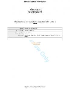
Potential Changes in Climate Due to Greenhouse Gases The impacts of climate change on agriculture will depend on the ultimate form of climate change, particularly the geographic pattern of temperature and precipitation changes. At present, it is impossible to predict such details of future climate with any confidence. The analyses in this report generally rely on climate projections generated by General Circulation Models (GCM’s). Generally, the studies reported here analyze climate scenarios from four equilibrium GCM simulations that show a doubling of carbon dioxide in the atmosphere.2 The four GCM runs are those of the Goddard Institute for Space Studies (GISS), the Geophysical Fluid Dynamics Laboratory (GFDL), the United Kingdom Meteorological Office (UKMO), and the Oregon State University (OSU) models. In some of the studies reported, other climate scenarios were used. Kaiser and others (1993) constructed a simple, statistically based weather generator. This allows construction of many different weather scenarios that show gradual warming over time consistent with a predetermined final temperature. While this approach is limited to the sites for which it was developed, it provides a way to generate time paths of climate change in the absence of such data from GCM runs. While equilibrium 2xCO2 scenarios have been standard model experiments reported from GCM’s, these experiments do not provide direct evidence of when these potential changes may occur. The timing of climate change depends on the specific path of CO2 concentration increase and climate system interactions with the ocean. In figure 1, we indicate how the global mean temperature change in 2xCO2 scenarios compares with the time path presented in IPCC (1996). These scenarios generally represent global temperature increases beyond what is expected by 2100. The exception is the OSU model where the global mean temperature change of 2.8° C is in the middle of range of temperatures expected by 2100. Regional changes in mean surface temperature and precipitation differ from the global means (table 1.1) and there are large differences in the pattern of change among the different GCM’s. (“Regional” will be used throughout the report to refer to a subset of the area under consideration. Here, we are referring to global climate variables, so “regional” means countries or groups of countries located together.) 2

To standardize results, GCM simulations consider a doubled preindustrial level of CO2 in the atmosphere (2xCO2).


3

There is general agreement among GCM predictions that higher latitudes will warm more than the global average and will receive disproportionately more precipitation, while midcontinental midlatitude areas may become drier, depending on the effects of aerosols (IPCC, 1996).

Figure 1

Global mean temperature rise Temp. rise (degrees C) 7 6 5

UKMO GISS

4

GFDL

The United States, Canada, and former Soviet Union/Mongolia data generally demonstrate these conclusions. For example, the hypothesized U.S. temperature increase is just slightly higher than the global mean and the relatively small increase in precipitation for the United States is likely to result in decreased soil moisture because of increased evaporation that accompanies higher temperatures. In comparison, temperature increases for Canada and the FSU/Mongolia are substantially above the mean, and precipitation increases, except for the OSU model, are much larger than the global land area mean. Tropical regions tend to show temperature increases slightly less than the mean temperature increase over the global land area. While there is some evidence to suggest that midcontinents become drier, precipitation

OSU

3 2 1 0 1990

2045

2100

Note: Projection of global mean temperature change from 1990 to 2100 for 3 climate sensitivities and a median emissions scenario including uncertainty in future aerosol concentrations, compared with 2xCO 2 General Circulation Model results for GISS, GFDL, UKMO, and OSU (see footnote, table 4.1). Source: Compiled by ERS from IPCC, 1996.

Table 1.1—Temperature (oC) and precipitation increase (percent) in four GCM’s for world regions GCM Region

OSU Temp. increase o

Global Land1 Regions2 U.S. Canada EC Japan Other East Asia Southeast Asia Australia/New Zealand Rest of the World FSU/ Mongolia Other Europe Other Asia Latin America Africa

C

GISS Precip.

Percent change

Temp. increase o

C

GFDL

Precip.

Percent change

Temp. increase o

C

UKMO

Precip.

Percent change

Temp. increase o

C

Precip.

Percent change

2.8 3.0

7 14

4.2 4.3

11 15

4.0 4.1

8 8

5.2 6.0

15 13

3.2 3.4 2.9 2.8 2.8 2.1 2.8

5 11 5 9 23 4 23

4.6 4.9 3.9 3.1 4.3 3.7 4.3

6 17 7 2 19 11 19

4.4 5.5 4.4 4.0 3.9 2.4 3.9

5 15 5 12 12 2 1

6.7 7.9 6.0 4.9 5.6 3.4 5.6

14 32 10 0 16 4 16

3.6 3.6 3.2 2.6 2.8

10 15 11 23 19

4.8 4.3 3.8 4.2 4.2

20 20 12 15 19

5.2 5.7 3.5 3.1 3.5

14 18 13 5 1

7.6 6.5 5.3 4.7 5.4

27 27 11 6 9

1

Global changes over land area only, excluding Antarctica. Regions as defined in Darwin and others (1995). Compiled by ERS and Roy Darwin based on results reported in Darwin and others (1995).

2

4


Table 1.2—Temperature and precipitation increase in four GCM’s for U.S. agricultural production regions GCM Region

OSU Temp. increase o

United States Northeast Lake States Corn Belt Northern Plains Appalachia Southeast Delta States Southern Plains Mountain States Pacific States Alaska Hawaii

C 3.2 3.2 3.5 3.5 3.2 3.5 3.4 3.4 3.3 2.7 2.3 3.7 2.5

GISS Precip.

Percent change 5 11 4 2 6 7 11 2 -2 -1 -1 24 2

Temp. increase o

C

GFDL

Precip.

Percent change

4.6 3.9 4.7 4.8 4.8 4.2 3.7 4.4 4.4 4.8 4.6 4.8 3.3

6 0 6 4 2 9 -1 -2 -6 11 15 14 2

Temp. increase o

C 4.4 4.6 4.7 4.3 4.4 4.0 3.7 3.9 4.0 4.4 3.9 5.1 2.9

UKMO

Precip.

Percent change 5 -2 12 6 6 3 6 6 -4 -1 7 20 1

Temp. increase o

C 6.7 7.6 8.3 7.2 6.7 6.6 5.5 5.8 5.9 6.3 6.2 7.9 3.7

Precip.

Percent change 14 16 11 8 12 7 6 -1 -4 19 20 37 31

Compiled by ERS and Roy Darwin based on results reported in Darwin and others (1995).

changes vary substantially across regions for each GCM. For all regions except the European Community, at least 10 percentage points separate the highest and lowest precipitation change predicted by different GCM’s. The OSU and GISS models predict that increased precipitation will fall more than proportionally on land, whereas the UKMO model predicts that proportionally more will fall over the ocean. By USDA farm production region, temperature changes vary less across regions and scenarios than does precipitation (table 1.2). The Southern Plains region shows a consistent precipitation decrease across GCM scenarios. The Lake States, Corn Belt, and Appalachia show a somewhat consistent precipitation increase of 5-10 percent. For other regions, the range of precipitation change is generally 10 percentage points or more between the largest and smallest increase. Agreement among these four scenarios should not be interpreted as lending a high degree of confidence to these projections because they are only four of an almost infinite number of GCM scenarios, any one of which has a number of limitations as predictions of future climate.


Carbon Dioxide and Its Direct Effect on Plant Growth Much of the work reported in subsequent chapters does not consider the direct effect of carbon dioxide (CO2) or other trace gases on plant growth. There is scientific evidence that CO2 increases plant growth and yields, even under open field conditions (Senft, 1995). For C3 crops (most crops other than corn, sorghum, and sugar cane), the estimated effect is a 30-percent increase in yield if carbon dioxide doubles; for C4 crops (corn, sorghum, and sugar cane), the effect is a 7-percent increase in yield (Kimball, 1983; Cure and Acock, 1986). Increased carbon dioxide levels also increase water use efficiency (Kimball, 1985; Woodward, 1993).3 Scientists studying the physiological effects of CO2 have raised a number of other issues. Plants may 3

Our reference scenarios are for an "equivalent-doubling" of carbon dioxide. Although projections of trace gas emissions suggest that carbon dioxide will be dominant, it is not the only contributor to increased upward pressure on temperature caused by the atmosphere (radiative forcing). Carbon dioxide is likely to contribute about 80 percent of the radiative forcing. Thus, we would expect a proportionately smaller yield effect than if CO2 provided all of the increased radiative forcing because other greenhouse trace gases have not been shown to contribute to plant growth.

5

adapt to higher CO2 over succeeding generations and may show a lower response over time. The quality, primarily the protein content, of grain and leaf may decline, meaning that the total food value of the harvest may not increase as much as the yield volume (Bazzaz and Fajer, 1992; Mooney and Koch, 1994). The photosynthetic effect of CO2 varies with temperature and other environmental conditions and, thus, the observed effect will not be equivalent at all locations (Van de Geijn and others, 1993). Increased CO2 may also make plants more resilient to some stresses. Finally, the effect is unlikely to be as strong if other nutrients are limited as may be the case in some developing countries, such as those in Sub-Saharan Africa, where fertilizer is often not available. The growth of weeds that compete with crops is also stimulated by CO2 fertilization.4 Issues and Uncertainties in Climate Change Projections The four GCM scenarios presented above are representative of possible climate changes under a doubled atmospheric CO2 climate, not predictions of future climate. The expertise to predict exactly a 5-percent chance that the global temperature will rise by more than 4°C by the year 2100 does not yet exist. Reviews of the state of scientific understanding of potential climate change point out several sources of uncertainty (Houghton and others, 1995; Houghton and others, 1992; IPCC, 1996; Schimmelpfennig, 1996). There is broad scientific agreement on many fundamental aspects of how human activities contribute to changes in the Earth’s climate. The radiative effect of increased levels of CO2 is well established. Natural levels of CO2 and water vapor maintain the mean surface temperature of the Earth at about 15°C; without them, the mean surface temperature would be about -15°C (Albritton, 1992). Gases like chlorofluorocarbons (CFC’s), methane, and nitrous oxide alter the radiative balance of the atmosphere (Houghton and others, 1992), and the atmospheric abundance of these gases has been increasing (Boden and others, 1994). Industrial activities that lead to emissions of CO2 and CFC’s are reasonably well measured and largely account for increases that have occurred since the late 1800’s. There is also little doubt that, without substantial changes in energy use, CO2 emissions will continue to increase. Together, these facts provide a strong case that CO2 emissions from the use of fossil fuels will contribute 4 For a general discussion of the CO2 fertilization effect, see Reilly (1992).

6

to warming. After more than a decade of research, consensus estimates of the increase in mean global surface temperature from doubling the level of CO2 in the atmosphere have not changed from the 1.5°C to 4.5°C initially reported by the NRC (1983). This is, however, a substantial range. If the mean temperature change is at the lower end of this range, most studies indicate minor or possibly beneficial impacts on agriculture. If, however, the mean temperature change is at the upper end of the range, some studies find more negative impacts on agriculture. Other uncertainties affecting assessment of agricultural impacts include: The global time path and local rate of global change. GCM results are better at describing a 2xCO2 world than the path taken to get there. Studies of climate change in the early 1980’s suggested the indicated scenarios might be observed by as early as 2030. This date has shifted as far forward as to 2100 as slower emissions growth and an ocean-thermal lag have been included in the models (fig. 1). Localized changes may be more rapid than the global average because geographic patterns can change while the global mean is changing. Changes in regular storm tracks could, over a few years, lead to greatly reduced rainfall in one area and increased rainfall in a new area. Gradual change spread over several decades would allow far more opportunities for adaptation. Changes in the daily and seasonal pattern of climate change. Given the magnitude of changes in the global system, there is no reason to believe that the daily, monthly, and seasonal patterns of temperature and precipitation will remain unaffected. Recent history shows an upward trend in nighttime low temperatures in the Northern Hemisphere but little or no change in daytime high temperatures (Kukla and Karl, 1993). Schimmelpfennig and Yohe (1994) estimate an index of crop vulnerability that provides a preliminary understanding of how changes in variability of climate affect production. Changes in the intensity of weather events. Heavy rain and high winds damage crops and cause soil erosion. Some scientific findings suggest that rainfall could become more intense with warmer temperatures (Pittock and others, 1991). The frequency and strength of regular weather cycles such as ENSO (El Niño Southern Oscillation) and the strength of the jet stream may change and thus change weather patterns. These factors and others leading to hurricanes, tornadoes, and hail and wind storms are not adequately modeled by coarse-resolution GCM simulations. These events have serious consequences


for agriculture; any increase in their frequency could have important effects not addressed in existing agricultural studies. Other factors not controlled for by GCM’s are: (1) there may be a natural trend in climate over a geologic time scale; (2) solar activity may influence climate trends; (3) stratospheric ozone depletion due to CFC’s may provide tropospheric cooling, partly offsetting warming due to greenhouse gases (Ramaswamy and others, 1992); and (4) sulfur emissions from burning coal may also offset warming (IPCC, 1996; Houghton and others, 1995). Sulfur emissions remain in the atmosphere only a few days and CFC’s are being phased out under the Montreal Protocol, so the greenhouse effect could be “unmasked” and accelerate warming in the near future. Unmodeled regional effects include wide-scale irrigation, deforestation, dust from tillage, and urbanization, which affect local temperature, precipitation, and insolation. While the combination of these effects may not have a significant effect on


the global change in mean temperature or precipitation, they could make a substantial difference to local areas when combined with longrun climate change. Climate Scenarios and Agricultural Impacts Despite the many uncertainties associated with climate forecasts, decisions are being made at the international level that require analysis of global food production. This report provides a synthesis of the best information available to support those decisions, given that many uncertainties exist. The results presented are quantitative, but the numbers merely facilitate the comparison of models to reach qualitative conclusions. The uncertainties associated with climate change impacts, compounded with uncertainty about the future, make it foolhardy to suggest that one set of numbers is right while another set is wrong. Abrupt changes in climate leading to agricultural catastrophes are not considered likely, while a rise in sea level is considered to affect only a small proportion of the world’s agricultural land. These factors, therefore, are not discussed here.

7