AIAA-98-4970 Multiobjective Optimization Using ... - Semantic Scholar

AIAA-98-4970 Multiobjective Optimization Using Adaptive Range Genetic Algorithms with Data Envelopment Analysis Masao ARAKAWA Dept. Mechanical Engineering and Science, Tokyo Institute of Technology. 2-12-1 Oookayama, Meguro, Tokyo 152-8552 Japan

Hirotaka NAKAYAMA Dept. Applied Mathamatics, Konan Univ. Okamoto, Higashinada,Kobe 658 Japan

Ichiro HAGIWARA Dept. Mechanical Engineering and Science

Hiroshi YAMAKAWA Dept. Mechanical Engineering, Waseda Univ. Ookubo, Shinjuku, Tokyo 169-8555

Abstract The present paper describe an implementation of the adaptive range genetic algorithms (ARange GAs) in multi-objective optimization by using the data envelopment analysis (DEA). ARange GAs is a new genetic search algorithms which adapt the searching range according to the optimization situation and make it possible to obtain highly accurate results effectively. DEA is to measure the efficiency of decision making units, and it is used mainly in the field of economy. When we combine both methods, we can obtain a great number of Pareto solutions, that might give an important aspect of the design, within a single GAs process effectively. The purpose of this study is to verify the characteristics and effectiveness of the proposed method through demonstrative examples.

Introductions Recently, requirements of design become more and more complicated and sophisticated and the customers try to decide what they really need to buy from many aspects. Thus, we need to satisfy multiple requirements to meet these purposes. In such cases, it is rational and natural to formulate the problem in the multi-objective optimization (MO). However, in MO, there usually exist conflict among objective functions, so that the solution cannot be determined uniquely. In general, we try to fine a set of non-inferior solutions call Pareto solutions with results of a number of scalar optimizations and try to give the implicit desired preference with local information and approximation of a given Pareto solutions. However, these processes are not that easy decision makings and we have to do many try and errors before we finally satisfy with the results, and which cause the cost of MO very high(1). When we try to think of the design as treasure hunting, these decision makings with local information seems to hunt treasure without a map. The map in MO might be a set of Pareto solutions, so that we would like to obtain

nearly entire set of Pareto solutions with almost the same computational cost with that we need in a single scalar optimization. One possibility to meet this complicated requirement is the use of genetic algorithms (GAs), because it can be considered as multi-point search. So that GAs seems to be preferable in MO. A number of studies have been done in using GAs in MO. Hajela (2) used weighted method to deal MO for structural system with mix of continuous, integer and discrete design variables. There are several studies which tried to keep Pareto solution as rank 1 and try to keep rank 1 individuals in the next generation, (3-6). The other is to divide population in a number of small groups(7) and try to maintain special characteristics in each small groups. Tamaki(8) combined these two approaches and obtained relatively good results. We have newly introduced a strategy for survival among phenotype expression as something of game between individuals and developed a new methodology(9), and we also have extended and revised the method to consider environment and use adaptive range GAs(10) to give evolution of the species(11). In this study, we also try to keep Pareto solutions and try to give higher fitness function for the frontier of Pareto solutions. We do not use ranking method like Goldberg or Fonseca, but to use DEA(12,13,14). DEA is an approach comparing the efficiency of decision making units (DMU) by measuring their efficiency by ratio of weighted sum of outputs and weighted sum of inputs. By using this efficiency measure, we can calculate DMU efficiency with in the range of [0,1] in continuous number. So that it might be suitable to use as fitness function in GAs. In this article, we demonstrate the proposed method by using simple numerical examples, and try to figure out the characteristics and effectiveness of the proposed method.

Adaptive Range Genetic Algorithms

The ARange GAs is developed by one of the au1 American Institute of Aeronautics and Astronautics

thor in order to treat continuous number effectively by using the same frame work of simple GAs. Details can be seen in the Refs. (10,15&16). Expression of continuous variables From the second generation, we can calculate mean (µi) and standard deviation (σi) of each design variable of the individuals who are remained after GAs processes. By using these values, we can determine some sort of distribution like normal distribution normalized to have maximum value 1 as N (xi ) = exp ( – (xi – µι)2 / 2 / σ 2ι ) (1). These distributions show situation of each generation and they adapt automatically to the best fitted searching range in some generation. By using these distributions, continuous variables are given as

(maxi – µι)2 (8) 2 log (LB) If there are any explicit side constraints for each design variable, there are possibilities that the searching ranges will break these constraints in the ARRange GAs. As we do not want to pass these problems in the fitness function as penalty, we operate both LB and s as following and keep side constraints. σi,new =

–

for upper bound

R(pi)=

– 2σ2ι ln LB +

LB i,new = UB – margin and 2

(UB– LB)C(pi) 2m – 1 – 1

µι+

(UB– LB)(C(pi)– 2 m – 1)

(2).

2m – 1 – 1

Where pi is the chromosome for design variable xi and C(pi) is the integer decoded by using gray coding, R(pi) is the real number decoded from pi, m is the number of bits, and UB and LB are system parameters. (See Fig. 1) In this method, searching range will move according to the value µi (mean value of the previous generation), thus we do not have to care on giving priori set boundaries. Moreover, if it comes close to convergence, distribution becomes narrow and it will speed up convergence. As the searching range will move according to the mean values of the previous generation, there is a possibility to miss the maximum variables, which have obtained during initial generation to previous generation, within the searching range. To avoid these situations, we make some efforts in the value σi as following and keep them in the searching range. previous range new range previous distribution LB 0 x0

x1

x2

µ x3

x4

(µι – lower i )2 2σ 2ι

LB i,new = exp

if LB i,new > UB – margin then LB i,new = UB – margin and

for C(pi)≥ 2 m – 1

1.0 UB

(3),

(upperi – µι) – 2log (LB i,new )

for lower bound

for C(pi) < 2 m – 1 – 2σ2ι ln UB–

2

if LB i,new > UB – margin then

σ i,new = µι–

(upperi – µι) 2σ 2ι

LB i,new = exp

x5

x x6

x7 R(pi)

Fig. 1 Illustrative sketch of adaptive range expression of continuous variables

σ i,new =

–

(µι – lower i )2 2log (LB i,new )

(4).

System parameters for ARange GAs There are five system parameters for ARange GAs; UB, LB, σmin, σmax and margin. And we give default values by assuming that the searching range will have the width of 10 as,{UB, LB, σmin, σmax,margin}={0.99, 0.044, 2.0, 0.1, 0.2}. However, these values must have different values according to the precision for each design variables. σmin and σmax will especially play important roles in improving accuracy. So that we give these values as, σmin=σmin *w /10.0 (5), σmax=σmax* w/10.0 (6), where w represent the width of searching range and it will be given by upper and lower bound for each design variables. If there are no side constraints, it can be determined by the initial given boundary. Expression of discrete variables In the conventional method, integer variable are determined by DI(pi)= xi,min+C(pi) (7), where xi,min is a priori set lower bound, as for discrete variable, they are DC(pi)=Database[[C(pi)]] (8), where Database[[k]] means number k-th discrete variable in the given set of discrete variables. In ARange GAs,

2 American Institute of Aeronautics and Astronautics

upperi

loweri

-2994.0

searching range fitness function

xi,min

µi

-2995.0

(a) normal case upperi

loweri

ARange=2994.49

searching range

Azarm=2994.57 -2996.0

xi,min

loweri

normal case µi

out of boundary (b) consideration of boundary upperi searching range

normal case µi

maxi xi,min (c) keep maximum value ever obtatined Fig.2 ARange GAs for integr and discrete variables xi,min is determined by the situation of the optimization using µ (Fig. 2), xi,min = Int(µi +0.5) - 2 m-1 (9), if xi,min < loweri then xi,min = loweri, else if xi,min + 2m -1 > upperi then xi,min = upperi - 2m + 1. Where Int(•) transforms real number to integer. To keep maximum value within the searching range, xi,min will be revised as, if xi,min > maxi then xi,min =maxi (10), else if xi,min + 2m+1 < maxi xi,min =maxi - 2m + 1. Demonstrative Example In order to show the effectiveness of the ARange GAs, we applied the problem to the Golinski’s speed reducer which was applied in Azarm(17). Here only the results is shown in Fig. 3 and Table 1. Formulation can also be seen in Web Page (http://fmad-www.larc.nasa.gov/ mdob/ mdo.test/class2prob4/descr.html). As you can see in Fig. 3 and Table 1, we have very good convergence and we can obtain the results which have high accuracy. After 750 generation, all 5 trials obtained the same results, which will proof the stability of the proposed

0

250

500

750

1000

generation Fig.3 Convergence of Golinski's speed reducer (5 trials)

Table 1 Comparison of the results in fitness function it trial 1 trial 2 trial 3 trial 4 trial 5 150 -2996.84 -3003.43 -2997.03 -2998.37 -2998.07 200 -2995.30 -2996.74 -2994.99 -2995.50 -2995.56 250 -2995.19 -2995.18 -2994.71 -2994.98 -2994.82 300 -2994.75 -2994.95 -2994.71 -2994.90 -2994.82 350 -2994.56 -2994.64 -2994.56 -2994.72 -2994.65 400 -2994.53 -2994.57 -2994.55 -2994.59 -2994.60 450 -2994.51 -2994.54 -2994.53 -2994.59 -2994.54 500 -2994.51 -2994.52 -2994.51 -2994.53 -2994.52 550 -2994.50 -2994.51 -2994.50 -2994.52 -2994.50 600 -2994.49 -2994.50 -2994.49 -2994.50 -2994.50 650 -2994.49 -2994.50 -2994.49 -2994.50 -2994.50 700 -2994.49 -2994.49 -2994.49 -2994.49 -2994.49 750 -2994.49 -2994.49 -2994.49 -2994.49 -2994.49 800 -2994.49 -2994.49 -2994.49 -2994.49 -2994.49 850 -2994.49 -2994.49 -2994.49 -2994.49 -2994.49 900 -2994.49 -2994.49 -2994.49 -2994.49 -2994.49 950 -2994.49 -2994.49 -2994.49 -2994.49 -2994.49 1000 -2994.49 -2994.49 -2994.49 -2994.49 -2994.49 method.

Data Envelopment Analysis General Formulation of DEA Data envelopment analysis (DEA) is first formulated by Charnes, Cooper and Rhodes (12). It provides a new definition of scalar efficiency of participating units, along with methods for objectively determining the weights by reference to the observational data for the multiple outputs and inputs that characterize such programs. In order to calculate efficiency of the units, we need inputs and outputs data of all the units which we would like to compare. The definition of efficiency is, s

θ=

Σuy i=1 m

i

Σvx j=1

j

i

(11), j

3 American Institute of Aeronautics and Astronautics

where xi= input data yi= output data vi=weight for input data xi ui=weight for output data yi m=number of input data s= number of output data θ= efficiency (called D eff. from now). When there are n decision making units (DMU), D eff of unit “o” can be calculated by;

Output 2 Input

D A

Frontier of efficiency E G

B

for unit "o", find ui o,vjo such that

Σ

OA efficiency θa= OP C P

F

s

max θo =

i=1 m

Σ

O

Σvx j=1

subject to

uio yio

uioyik

Σvx j=1

≤ 1 (k = 1,...,n)

(12),

jo jk

ui o 0 (i=1,...,s) vj o 0 (j=1,...,m) where subscript “o” is efficiency and weights for unit “o” and “k” is data for unit “k”. Eq. (12) can be converted into linear programming and by using dual method, it can be rewritten as,

find θo and λo such that max θo subject to θoxo – Xλ o ≥ 0 yo – Yλ o ≤ 0 λo ≥ 0 where

units Output 1 Input

Fig. 4 Illustrative explanation of DEA with 1 input and 2 outputs

jo jo

s

i=1 n

H

given in Fig. 4, and when θo=1.0, it means the unit “o” is located at the frontier of the efficiency. Remarks Many advantages are reported in the refs (11,12) by using the results of DEA. However, we only need to calculate efficiency in this study. So that we are loosing many other advantages in DEA. Even though, we can benefit some of the advantages; 1.We do not have to care the order of given data. 2. We can obtain efficiency in scalar value. And it shows how far the reference data will be from the frontier. 3. When optimization process goes by, frontier of the efficiency will become a set of Pareto solution. Only the lack in DEA is that it assume the convex nature of the frontier. Which means we cannot measure efficiency correctly when there are concave nature in the Pareto optimum solution sets.

Multi-objective Optimization in GAs

λ o: Lagrange multiplier θo : efficiency xjk : input data sets yik : output data sets

(13)

. Each data has its specific meaning, like the determined weights mean that the weight which give highest efficiency, Lagrange multipliers means to determine superior sets and the direction of improvement and so on. But in this study, we only need efficiency θo, thus we do not go into the detail any more, Illustrative explanation is

Here we only give a formulation of multi-objective optimization and present the conventional way to estimate fitness function by using ranking strategy. Formulation Find x such that minimize F(x)={f1(x),..., fL(x)}T subject to gj(x) ≥ 1.0 xiL ≤ xi ≤ xiU, where x= design variable (={x1,..., xN}T)

4 American Institute of Aeronautics and Astronautics

(14)

F(x)= objective functions(={f1(x),..., fL(x)}T) gj(x)= constraints (j=1,...,M) xiL ,xiU= side constraints

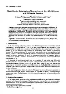
method, even if individual E has ranking 1, it is almost the same distance with F from the frontier which is determined by DEA. It seems very strange and it will cause zigzag Pareto solutions for the result of GAs.

Penalty function In GAs, we cannot treat constraints. So that we have to include them into fitness function using penalty functions. pj × P[1.0 – g j (x)]a Σ j =1 M

peni (x) = fi (x) +

(15),

where pj= penalty coefficient a= penalty exponent

P[y]=

y for y > 0 0 otherwise

(16).

By using Eq. (15), we can convert them into fitness function (fiti) for each objective function. (Usually fitness function will be maximize in GAs.) Ranking method By using the penalty function for each objective function, we would like to give higher fitness value to the frontier to apply GAs. One of the method is ranking method(3). We will illustrate how we rank each individuals in Fig. 5. In this method, count the number of individuals which has higher fitness value for every fitness function and add 1 to its number. For example, individual D has no individual which has higher objective function of both fit1 and fit2, thus its ranking is 1. Individual 4 has 2 individuals (G and H), thus its ranking is 3. In this

fit 2

D A (2)

In the proposed method, we try to estimate fitness value by using DEA. We have to prepare data for DEA. Input in DEA will be the objective function which we would like to minimize and output will be the objective function which we would like to maximize. So it might be straight forward after we calculate objective functions and constraints and convert them in to fitness function using Eq. (15). However, there are some conditions in DEA that we have to convert data for its purpose. Preparation of data 1. In DEA, we need at least two input and one output (or one input and two output) data. If we do not have enough data, add unit data set for output data. 2. In DEA, all data need to be plus, thus, when there are minus value in the fitness function, convert fitness function value as, (17), fiti=fiti - min(fiti)+ε where ε is a small number. (ε=0.1 in the following examples) Flow of the proposed method Flow of the proposed method is shown in Fig. 6. Randomly create initial population decode them by using conventional method Add every data sets to estimation sets and calculate behavior variables

DEA's frontier C (1)

The proposed method

0 individual -> rank =1

store θ> t individual data to estimation sets

generation max generation end

GAs process yes

B (5)

no

yes

0 individual -> rank =1 E G (1) H (1) F 2 individuals -> rank =3

DEA to calculate fitness function

generation AR generation yes determine the new searching range by giving µi and σi

O

fit 1 Fig. 5 Illustrative explanation of DEA with 1 input and 2 outputs

decode them by using ARange method

Fig. 6 Flowchart of the proposed method

5 American Institute of Aeronautics and Astronautics

Initially, populations are given randomly and decode by using conventional GAs. We prepare data for DEA and calculate fitness function. If fitness function is nearly equal to 1 (> t), we store them into DEA calculation data. Simple GAs will be ran for several times with conventional decoding method for a while (10 generation in the following examples). In this process we would like to find global information of the frontier. After that we will use ARange decoding. Unfortunately, mean value does not have any importance like it has in the single objective optimization case. So we determine its value by following. We repeat the process until generation become maximum generation. Determination of a new range In ARange decoding, a new searching range will be determined by µi and σi. However, because there are many different objectives, mean value does not have any important meaning. What we would like to have in MO is a precise set of Pareto solutions. Thus, we would like to give searching range near the Pareto solutions. First, we will find two individuals (a and b), which is in the neighbor and has maximum distance (Fig. 7), Then, µi is determined as,

µ i = w xi,a + (1 – w) xi,b

(18)

where w is a parameter randomly given by [-0.25, 1.25] in the following. Then, σi is determined by the conventional ways. By using these ranges, we can fill the Pareto solutions which are given by using conventional decoding method. Counter-plan for concave characteristics In DEA, we only can solve convex characteris-

x2 1

no other frontier data 3

tics. When we have any pre-knowledge or we found that there are any concave characteristics in the frontier, we can convert them to convex character by using following equation. fiti=Exp(fiti) (19) Although it is only a counter-plan for concave characteristics, if we can give some good weight for them, we can solve concave characteristics problem like we can see in Athan and Papalambros(18).

Demonstrative Examples Tamaki’s simple problem In order to show the effectiveness of the proposed method, we carry out a simple numerical example shown in Tamaki(7). Minimize f1(x1,x2) = 2 x21 – x2 and f2(x1,x2) = – x1 subject to (20) (x1 – 1)3 + x2 ≤ 0 (x1,x2) = ([0,),[0,)) To show the effectiveness of the proposed method, we compare the results with cases. Case 1: Fonseca’s method with conventional decoding Case 2: Fonseca’s method with old ARange decoding Case 3: DEA with conventional decoding Case 4: DEA with new ARange decoding Case 5: DEA with Eq. (19) with conventional decoding Case 6: DEA with Eq. (19) with new ARange decoding In the conventional decoding, we use 6 bits for each design variables, and in ARange decoding we use 4 bits for each design variables. And AR generation equals to 10. Results of each case in the design variable is shown in Fig. 8 to 12. Comparison of the results in objective function space of case 4 and 6 is shown in Fig. 13. In case 1, we can obtain over all Pareto solution sets after 100 generations. But the results include zigzag relations, which can be seen explicitly in the results after 30 generation. In that sense, we have to examine the results, which are good Pareto solution and which are not. 1.0

1.0

4 Maximum distance µ 1 = w x1,3 + (1 – w) x1,4 µ 2 = w x2,3 + (1 – w) x2,4

O

dv2

dv2

2

x1 Fig. 7 Determinatio of the searching range

0.0

0.0 0.0

1.0

0.0

1.0

dv1 dv1 after 30 generation after 100 generation population Rank 1 data Fig. 8 Results of Case 1

6 American Institute of Aeronautics and Astronautics

1.0

1.0

1.0

dv2

dv2

dv2

0.0 1.0

0.0

1.0

0.0

1.0

0.0

f2 -0.6

0.0 0.0

1.0

0.0

1.0

dv1 dv1 after 30 generation after 100 generation population efficient frontier data Fig. 10 Results of Case 3 (t=0.995) 1.0

D eff > 0.999

1.0

Concave part

f2 D eff > 0.995

0.0

1.0

dv1 dv1 after 30 generation after 100 generation population efficient frontier data Fig. 13 Results of Case 6 (t=0.999) 0.0

dv2

dv2

0.0

1.0

dv1 dv1 after 30 generation after 100 generation population Rank 1 data Fig. 9 Results of Case 2 1.0

dv2

0.0

0.0 0.0

1.0

-1.2 -1.5

0.0 1.5 2.5 f1 Case 4

0.5 0.0

4.0 f1 Case 6

8.0

Fig. 14 Comparison of the results in objective function space

1.0

dv2

dv2

0.0

0.0 0.0

1.0

0.0

1.0

0.0

1.0

dv1 dv1 after 30 generation after 100 generation population efficient frontier data Fig. 11 Results of Case 4 (t=0.995) 1.0

1.0

dv2

dv2

0.0

0.0 0.0

1.0

dv1 dv1 after 30 generation after 100 generation population efficient frontier data Fig. 12 Results of Case 5 (t=0.999) In case 2, we use old ARange decoding that is to use mean value. We can see that zigzag nature is exaggerated and it would not disappeared after 100 generation, because the searching range became so narrow to search the other possibility. In that sense, usage of old ARange in Fonseca’s method was failed. In case 3, even the results after 30 generation, we have obtained data in need to predict the actual Pareto solution sets. After 100 generation, we have

a good set of Pareto solutions without zigzag nature. Which mean that we only have the data in need. However, the data between x1=[0.1,0.2] is missing. In Fig. 11, we can see that the proposed ARange tried to find the results of missing part in case 3. As ARange can have more precision that it can obtained some missing part of case 3 and obtained over all Pareto optimum sets. When we use convex conversion of fitness function, we can obtain the missing part of case 3 even with the conventional decoding (Fig. 12). In Fig. 13, we can obtain more Pareto solution than in case 5. Even in the result after 30 generation, we can obtain almost the same number of Pareto solutions which is obtained after 100 generation in case 5. Compared with the results with case 4, we can obtain more precise Pareto sets. This results are quite natural, because DEA can estimate its efficiency more accurate in the convex case. As we can see in Fig. 14, the problem has some concave character in its Pareto solution sets. Thus, there are some missing part in the original method. However, after converted to the convex problem, we can obtained all over the Pareto solution precisely. A static three-bar truss problem The problem is first solved by Koski(19) and it is also used to explain the efficiency by Athan and Papalambros (18). The total volume of the truss and a linear combination of the two nodal displacements are to be minimized. The design variables are the three cross sectional area of

7 American Institute of Aeronautics and Astronautics

A1

1.00

A3

A2

10-3

10-3

3L

L

1.00

population D eff>0.9999 jump

population D eff>0.9999 jump

V(m3)

V(m3)

L F

dv

0.00

dh F Fig. 15 Three-bar truss under static loading

10-3

1.00

the members. Stress and side constraints are imposed. The three bar truss is shown in Fig. 15. Problem formulations are as follow;

-3

-3

10 10 1.50 2.50 0.50 1.50 2.50 0.00 0.50 Displacement (m) Displacement (m) After 30th generation After 100 generation Fig. 16 Results in the case we do not use Eq. (19)

10-3

1.00 population D eff>0.999999

population D eff>0.999999

jump V(m3)

jump

V(m3)

Find {A1,A2,A3} such that minimize V

=

2LA1 + LA2 + 2LA3

(21)

and d=0.25 dv + 0.75 dh subject to σc ≤ σ ≤σt (i=1,2,3) AL ≤ A ≤ AU (i=1,2,3), where

0.00

10-30.00

0.50 1.50 2.50 Displacement (m)

10-3

0.50 1.50 2.50 Displacement (m)

After 30th generation After 100th generation Fig. 17 Results in the case we use Eq. (19)

some missing range on design variable space, so that the searching range will become those range where there seems no Pareto solutions like we can see in the circle of Fig. 17. This might be one of the shortcoming of using Eq. (18). However, even in the results after 30 th generations, we can predict the over all Pareto solution sets sufficiently, and it shows effectiveness in the searching of the solutions of the proposed method. Comparing the both results, convex conversion results seems to obtain Pareto solutions more effectively. Even we give higher “D eff” value, we obtained more Pareto solution than the other. This is quite natural results, because of the nature of DEA that need convex characteristics in the objective functions.

dv = 8FL b2 – d E b – ad dh = 8FL b2 – a E b – ad E(dv – dh ) σ1 = 2L Edv σ1 = L E(dv + 3dh ) σ1 = 4L

Conclusions

a = 8A2 + 8A1 + A3 b = 3A3 – 8A1 d = 3A3 + 8A1 F=20KN, L=1.00m,E=200GPa, σt=200MPa, σc=-200Mpa AL=1.0 e-5 m2, AU=2.0 e-4 m2 We applied the proposed method in both case with convex conversion and without convex conversion. Results are shown in Figs. 16 & 17. In the both cases, we have obtained sufficient number of Pareto solutions, in order to predict over all Pareto solution sets. Although the problem seems to have a convex character, there are some jump in the Pareto sets, because even if we convert the problem to convex character they do not vanish. In such a case, Eq. (18) try to search the range which are

1. In this article, we proposed a new multi-objective optimization method, using ARange GAs with DEA. 2. When we use ARange decoding, we do not have to care about the initial searching range and the number of bits to determine precision of the results. As ARange decoding try to adapt the searching range adaptive to the range where we would like to obtain solutions and when the convergence goes by, it will narrow the range to obtain more precise results. 3. DEA gives some mathematical meaning for Pareto optimality. In these sense, we can give rational fitness function to each individuals, so that we can avoid to obtain some zigzag nature which will cause by estimating Pareto optimality with conventional ranking methods. Moreover, efficiency in DEA will be much more suitable for GAs. 4. Through some simple numerical examples, we showed

8 American Institute of Aeronautics and Astronautics

the effectiveness of the proposed method. One of the shortcoming in using DEA is that they cannot treat the problem with concave case, We proposed one counterplan to convert the problem into convex characteristics and obtained the results much better than the original ones. 5. In the proposed method, we can obtain enough number of Pareto solutions to predict over all Pareto solutions sets within relatively small number of generations. Which will show the effectiveness of the proposed method in the stand point of convergence. We still need some effort to give searching range to obtain the over all Pareto solutions. We would like to investigate that point in the future.

Acknowledgments This is a part of the study done in the project of “Collaboration Laboratory” in Tokyo Institute of Technology endowed by East Japan Railway Co., it is also supported by Japanese Science promotion fund (#09450100). Their support are greatly acknowledged. We also would like to appreciate for the discussion and advice from Prof. H. Sugimoto at Hokkai Gakuen Univ.

References (1) Nakayama, H, “ On Applications of Multi-objective Programming”, Proceedings of the Sixth RAMP Symposium., (1994), p. 135-149, (in Japanese). (2) Hajela,P., Lin, C.-Y., “Genetic Search Strategies in Multicriterion Optimal Design”, Structural Optimization, Vol.4, (1992), p.99-107. (3) Goldberg, D. E, Genetic Algorithms in Search, Optimization, and Machine Learning, Addison-Wesley., (1989). (4) Fonseca, C.M. and Fleming, P.J., “ Genetic Algorithms for Multi-objective Optimization : Formulation, Discussion and Generalization”, Proceeding of the Fifth International Conference on Genetic Algorithms, (1993), p.416-426. (5) Osyczka, A. and Kundu, S., “An Approach to Design Optimization Using Evolutionary Computation Technique”, Proceeding of the Second China- Japan Symposium on Optimization of Structural and Mechanical Systems, (1995), p.158-165. (6) Belegundu, A.D. , et. al., “ Multiobjective Optimization of Laminated Ceramic Composites Using Genetic Algorithms”, Collection of Technical Paper on 5th Multidisciplinary Analysis and Optimization, AIAA, (1994),1015-1022. (7) Schaffer, J.D., “ Multiple Objective Optimization with Vector Evaluated Genetic Algorithms”, Proceeding of the First International Conference of Genetic Algorithms and Their Application, (1985), p.93-100. (8)Tamaki,H., “ Multi-Criteria Optimization by Genetic

Algorithms”, Chap. 3 on “Genetic Algorithms 2 (edited by Kitano), Sangyotosho, (1995), p.71-87. (9) Arakawa, M, Yamakawa, H., “Strategic Genetic Algorithms to Obtain Multiple Acceptable Design”, in CD-ROM proceeding of 22nd Design Automation Conference, (1996). (10) Arakawa, M., Hagiwara, I., “Development of Adaptive Real Range Genetic Algorithms”, JSME International, to be appeared. (11) Arakawa, M., Hagiwara, I., Yamakawa, H.,"Foraging Strategic Genetic Algorithms To Obtain Multiple Acceptable Designs", Proc. on Int. Symp. of Optimization and Innovative Design 97, (in CD-ROM), (1997) (12) Charnes, A., Cooper, W.W,. Rhodes, E., “ Measuring the efficiency of decision making units”, European Journal o fOperation Research , Vol.2, (1978), p. 429444. (13) Boussofiane,A., Dyson, R.G., Thanassoulies E., “Applied Data Envelopment Analysis”, European Journal of Operational Research, Vol, 52, (1991), p.1-15. (14) Tone,K., “Data Envelopment Analysis”, Nikkagiren, (1993), (in Japanese) (15)Arakawa,M. & Hagiwara,I.,"Nonlinear Integer, Discrete and Continuous Optimization Using Adaptive Range Genetic Algorithms",Proc. of Design Technical Conference (in CD-ROM),ASME, (1997) (16)Arakawa,M. & Hagiwara,I.,"Development of Adaptive Range Genetic Algorithms(Proposal of the new operators for efficient and high accurate solutions)",Proc. of OPTIS98, JSME, (1998) to be appeared in Japanese. (17)Azarm, S., Papalambros, P. ,Tran. of ASME, Journal of Mechanisims, Transmissions, and Automation in Design, Vol. 106, No.1, (1984), pp.82-89. (18) Athan, T.W., Papalambros, P.Y., “A Note on Weighted Criteira Methods for Compromise Solutions in MultiObjective Optimization”, Eng. Opt., Vol, 27, (1996), p. 155-176. (19) Koski, J., “Defectivenss of Weighting Method in Multicriteira Optimization of Structures”, Communications in Applied Numerical Methods, Vol. 1, (1985), p.333-337.

9 American Institute of Aeronautics and Astronautics