Multiobjective Optimization by Decomposition with ... - Semantic Scholar

Multiobjective Optimization by Decomposition with Pareto-adaptive Weight Vectors Siwei Jiang1,2 , Student Member, IEEE, Zhihua Cai2 , Jie Zhang1 , Yew-Soon Ong1 School of Computer Engineering, Nanyang Technology University, Singapore1 School of Computer Science, China University of Geosciences, Wuhan, China2

Abstract—MOEA/D is a recently proposed methodology of Multiobjective Evolution Algorithms that decomposes multiobjective problems into a number of scalar subproblems and optimizes them simultaneously. However, classical MOEA/D uses same weight vectors for different shapes of Pareto front. We propose a novel method called Pareto-adaptive weight vectors (paλ) to automatically adjust the weight vectors by the geometrical characteristics of Pareto front. Evaluation on different multiobjective problems confirms that the new algorithm obtains higher hypervolume, better convergence and more evenly distributed solutions than classical MOEA/D and NSGA-II.

I. I NTRODUCTION Many real-world problems can be described as Multiobjective problems (MOPs). MOPs always have several conflict objectives, and it is difficult to simultaneously optimize all the objectives. The tradeoff point is a Pareto-optimal solution, the set of Pareto-optimal solutions is called the Pareto Set (PS), and the set of all Pareto-optimal objective vectors is the Pareto front (PF). Multiobjective Evolutionary Algorithms (MOEAs) are demonstrated to be suitable for solving various complex MOPs [1]. Currently, most MOEAs are Pareto dominance-based algorithms such as NSGA-II [2], SPEA2 [3], SMPSO [4]. These algorithms use the Pareto dominance relation together with a crowding distance or neighbor density estimator to evaluate individuals. Pareto dominance-based algorithms work generally well to approximate PF in two or three objectives. However, the performance is severely deteriorated by the increasing number of objectives, because almost all the solutions are nondominated by each other under many objectives. MOEA based on decomposition (MOEA/D) belongs to another scope to solve MOPs, which decomposes multiobjective problems into a number of scalar subproblems and optimizes them simultaneously. Classical MOEA/D mainly includes three decomposition approaches: weighted sum, weighted Tchebycheff [5] and boundary intersection [6]. A new penaltybased boundary intersection (PBI) approach is proposed in [7]. MOEA/D has several advantages over Pareto dominancebased algorithms such as computational efficiency, scalability to many problems and high search ability for combinatorial optimization problems. Despite its advantages, MOEA/D has two limitations: (1) MOEA/D is unable to produce an arbitrary number of weight vectors when the number of objectives is larger than two; (2) the weight vectors in classical MOEA/D are unchanged for different shapes of PF.

We propose a novel method called Pareto-adaptive weight vectors (paλ), inspired by the Pareto-adaptive ϵ-dominance method that divides the objective space into different sizes of hyper boxes according to the geometrical characteristics of Pareto front [8]. The paλ approach has two important features: (1) paλ is based on Mixture Uniform Design (MUD) and able to generate an arbitrary number of weight vectors even when the number of objectives is larger than two; (2) paλ is driven by the hypervolume metric. It can automatically adjust weight vectors to scatter for concave PF, whereas assemble weight vectors for the convex PF. Experimental results on various multiobjective problems show that paλMOEA/D obtains higher hypervolume, better convergence and more evenly distributed solutions than classical MOEA/D and NSGA-II. II. paλ: PARETO - ADAPTIVE W EIGHT V ECTORS The paλ is based on Mixture Uniform Design, and it automatically adjusts weight vectors by the shape of PF. A. Weight Vectors by MUD m−1 For MOEA/D, the number of weight vectors N = CH+m−1 is controlled by the parameter H. When the number of objectives m is larger than 2, N is a discrete sequence for different H. paλ adopts Mixture Uniform Design (MUD) to produce an arbitrary number of evenly distributed weight vectors when m ≥ 3. MUD is an advanced experimental design method. Suppose that a vector is composed of m components x1 , · · · , xm . Each vector is one point in the space region T m = {(x1 , · · · , xm ) : xi ≥ 0; i = 1, · · · , m; x1 + · · · + xm = 1}. The opinion of MUD is to evenly spread the N experimental points (representing the N vectors) in region T m . The detailed algorithm can be found in [9]. For example, in the case of N = 10 and m = 3, MUD first constructs an uniform design array U10 (102 ), and then transfers U m−1 to C m−1 cubic space. The weight vectors λk = (xk1 , xk2 , xk3 ), k = 1, · · · , N can √ √ be calculated as: xk1 = 1 − ck1 , xk2 = ck1 (1 − ck2 ), and √ xk3 = ck1 ck2 .

B. paλ for Two, Three and more Objectives paλ controls weight vectors to assemble or scatter depending on the geometrical characteristics of PF. We first illustrate paλ in the bi-objective case. Assuming that PF is symmetric and the m objectives are normalized to 0 ≤ fi ≤ 1. The curve

hv(λ) = 0.774252 ; 10 Points along Pareto front 2: f0.5 + f0.5 =1 1 2 hv(λ) = 0.169539 ; 10 Points along Pareto front 1: f2.0 + f2.0 =1 1 2

hv(paλ) = 0.793305 ;10 Points along Pareto front:f0.5 + f0.5 =1 1 2

1

0.8

1 Pareto front λ Lines Intersection points

0.9

Pareto front λ Lines Intersection points

0.9

hv(paλ) = 0.178965 ;10 Points along Pareto front:f2.0 + f2.0 =1 1 2

1

Pareto front λ Lines Intersection points

0.9

0.8

0.8

0.7

0.7

0.6

0.6

0.5

0.5

0.7

f2

f2

f2

0.6 0.5 0.4

0.4

0.3

0.3

0.2

0.2

0.2

0.1

0.1

0.4 0.3

0

0

0.2

0.4

0.6

0.8

1

0

0.1 0

0.2

0.4

f1

0.8

1

0

0

0.2

0.4

f1

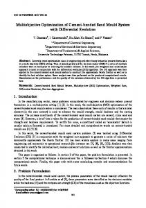
(a) λ (MOEA/D) for convex and concave PF Fig. 1.

0.6

0.8

1

f1

(b) paλ for convex PF

(c) paλ for concave PF

10 Intersection Points along 2-dimensional Pareto Front by λ (MOEA/D) and paλ Method

of PF can be represented as f1p + f2p = 1. The weight vectors satisfy λ1 + λ2 = 1, whose gradients are represented by λ lines (Figure 1). These λ lines produce N intersection points along PF. To evaluate the distribution of such points, we set the hypervolume metric [10] as a rule to drive paλ method. When p = 1, the shape of PF is a line f1 + f2 = 1, the λ lines are distributed perfectly, and the set of intersection points has the maximum hypervolume. When p ̸= 1, we need to move the intersection points until they are evenly distributed along f1p + f2p = 1. In other words, the intersection points with the maximum hypervolume is the ultimate goal. paλ introduces a scale parameter l to adjust the gradient of λ lines: ff21 = ( λλ21 )l . Define the intersection points as {(xi1 , xi2 ), i = 1, · · · , N }. They are along PF and on the adjusted λ lines: (xi1 )p +(xi2 )p = xi λi 1; xi2 = ( λ2i )l . 1 1 For an assumptive scale parameter l, a set of intersection points is calculated by solving the above equations. Then, the hypervolume of such points is associated with the parameter l. paλ adopts Simplex Method to find evenly spread intersection points with the maximum hypervolume. The Simplex Method repeatedly uses the shrink, reflection and expansion procedures to get the optimal scale parameter lopt . After that, the adjusted weight vectors can be calculated as: λi

λipaλ

0.6

opt

(1, ( λi2 )l ) xi xi 1 =( i 1 i, i 2 i)= λi2 lopt x1 + x2 x1 + x2 1 + ( λi ) 1

Figure 1 shows an example of 10 intersection points along PF generated by λ (MOEA/D) and paλ respectively. When p = 0.5, the hypervolume of the intersection points is hv = 0.774252 by MOEA/D (plot (a) in Figure 1). From plot (b) in Figure 1, paλ gets the optimal parameter lopt = 1.7105 and larger hv = 0.793305, the λ lines are scattered in the objective space, and the intersection points are moved to the two endpoints of PF. When p = 2, the hypervolume of intersection points is hv = 0.169539 by MOEA/D. paλ gets the optimal parameter lopt = 0.56192 and larger hv = 0.178965 (plot (c) in Figure 1). λ lines are assembled together in the objective space, and the intersection points are moved to the median of PF.

For the tri-objectives case, paλ sets the number of scale parameters as 2. The λ lines are adjusted in two directions: in the plane xy the λ lines are adjusted by parameter l2 , and in the plane xz the λ lines are adjusted by parameter l3 . The intersection points along Pareto front and on the adjusted λ lines (i = 1, · · · , N ) can then be defined as: (xi1 )p + (xi2 )p + (xi3 )p = 1;

λi xi λi xi2 = ( 2i )l2 ; 3i = ( 3i )l3 i x1 λ1 x1 λ1

The two parameters l2opt , l3opt are optimized by the Simplex Method, and the adjusted weight vectors are calculated as: λi

λipaλ

opt

λi

opt

(1, ( λi2 )l2 , ( λ3i )l3 ) (xi , xi , xi ) 1 1 = i 1 2i 3 i = λi opt λi opt x1 + x2 + x3 1 + ( λi2 )l2 + ( λ3i )l3 1

1

paλ can expand to the case of more than three objectives. The scale parameters (l2 , · · · , lm ) are set for m objectives. At first, the weight vectors {λi = (λi1 , · · · , λim ) : i = 1, · · · , N } are initialized by MUD. Then, we estimate the p value of PF [8]. Finally, the scale parameters are optimized by the Simplex Method. The Pareto-adaptive weight vectors can then opt be calculated as follows: rji =∑ (λij /λi1 )lj (j = 2, · · · , m) and m i )/(1 + j=2 rji ). λipaλ = (1, r2i , · · · , rm III. T HE paλ-MOEA/D A LGORITHM The paλ-MOEA/D algorithm is based on decomposition with Pareto-adaptive weight vectors, and its decomposition method is the Tchebycheff approach. A pseudo code of paλMOEA/D is given in Algorithm 1. Some parameters are defined as: N is the size of population; T is the number of the neighborhood for weight vectors; Archive is the external population which stores the non-dominated solutions. There are four steps in the paλ-MOEA/D: Step 1 is to initialize the first population, weight vectors, neighborhood and the external population (Archive); Step 2 is to generate the next offsprings, update population and Archive; Step 3 is the paλ method (as described in Section 2); and Step 4 is to quit the algorithm when the number of fitness function evaluations is larger than max evals.

To explain, the initial weight vectors are generated by the Mixture Uniform Design (Line 5). As mentioned in Section II-A, by adopting MUD, we can generate an arbitrary number of weight vectors even when the number of objectives is larger than two. This expands the scalability of MOEA/D. The paλ method is implemented as Lines 14-21. In Line 18, paλ estimates the parameter p of the Pareto-optimal front p = 1 by calculating the area of non-dominated f1p + · · · + fm solutions in Archive [8]. In Line 19, paλ is driven by the hypervolume metric (As described in section II-B). A larger hypervolume means that the intersection points distribute more evenly along the PF. paλ automatically adjusts the intersection points to scatter when PF is convex but assemble when PF is concave. There are m − 1 parameters to be optimized for m objectives by the Simplex Method. In Lines 20-21, the new weight vectors are used to update the neighborhoods of each weight vector. The algorithm finally outputs the non-dominated solutions in population when the stopping criteria is satisfied (Lines 2325), which form the solutions of the multiobjective problem.

1 2 3 4 5 6 7 8 9 10

11 12 13

14 15 16 17 18 19 20 21

Algorithm 1: The paλ-MOEA/D Method Step 1: Initialization Method Set evals = 0, f lag = f alse; Random generate first population X; Evaluate X and update evals; Generate first weight vectors λ by MUD; Compute the T neighborhoods for every λ; Add X into Archive by dominance relationship; Step 2: Update Procedure for i = 1, · · · , N do Generate a new solution y ′ from X by DE operator and polynomial mutation; Evaluate y ′ and evals + +; Update population; Add y ′ to Archive by dominance relationship; Step 3: Pareto-adaptive λ Method if f lag == true or |Archive| < 2N then Go to Step 4; Set f lag = true; Estimate parameter p of Pareto front for Archive; Pareto-adaptive weight vectors; Get the new weight vectors λ = λpaλ ; Recompute T neighborhoods for every λ;

24

Step 4: Stopping Criteria if evals < max evals then Go to Step 2;

25

Output the non-dominated solutions in X.

22 23

IV. E XPERIMENTAL R ESULTS AND D ISCUSSION Experimental study to evaluate paλ-MOEA/D against other competing approaches using jMetal 3.0, a Java-based framework that is aimed at facilitating the development of metaheuristics for solving MOPs, on benchmark problems.1 A. Test Problems and Experimental Setting The test problems are ZDTx and DTLZx. ZDTx problem family include five bi-objective problems (ZDT1, ZDT2, ZDT3, ZDT4 and ZDT6). DTLZx problem family include seven tri-objective problems (DTLZ1, DTLZ2, DTLZ3, DTLZ4, DTLZ5, DTLZ6 and DTLZ7). Five algorithms are tested including one Pareto dominancebased algorithm and four decomposition-based algorithms: NSGA-II, Non-Dominated Sorting Genetic AlgorithmII [2]; MOEA/Dws , MOEA/D with the weight sum approach; MOEA/Dte , MOEA/D with the Tchebycheff approach [5]; MOEA/Dpbi , MOEA/D with the penalty-based boundary intersection approach [7]; and paλ-MOEA/D, MOEA/D with Pareto-adaptive weight vectors. The parameter settings are outlined as follows. The population size is 25 for ZDTx and 105 for DTLZx respectively. The number of weight vectors for the tri-objective problems m−1 2 = 105 in classical MOEA/D can be drew CH+m−1 = C13+2 when H = 13. The number of fitness function evaluations is 25, 000 for ZDTx and 50, 000 for DTLZx. Every algorithm launches 100 times independently for each test problem, to obtain statistically significant results. The number of neighborhoods T is 20. For DE (Differential Evolution) operator CR = 1.0 and F = 0.5. The probability of SBX crossover is 0.9. For polynomial mutation, η = 20 and pm = 1/n, where n is the number of decisional variables. We adopt five performance metrics: Hypervolume, Inverted Generational Distance (IGD), Generational Distance (GD), 1 Unary Additive Epsilon Indicator (Iϵ+ ) and Spread. The higher 1 and Spread indicate the Hypervolume and lower IGD, GD, Iϵ+ better performance. Results are compared using median values and the superior results of test problem are highlighted as grey background. TABLE I M EDIAN OF H YPERVOLUME (HV)

ZDT1 ZDT2 ZDT3 ZDT4 ZDT6 DTLZ1 DTLZ2 DTLZ3 DTLZ4 DTLZ5 DTLZ6 DTLZ7

MOEA/Dws MOEA/Dte MOEA/Dpbi NSGA-II paλ-MOEA/D 6.521e − 01 6.392e − 01 6.057e − 01 6.381e − 01 6.412e − 01 0.000e + 00 3.097e − 01 2.957e − 01 3.060e − 01 3.107e − 01 4.863e − 01 4.870e − 01 4.642e − 01 5.066e − 01 4.873e − 01 3.534e − 01 6.360e − 01 6.244e − 01 6.359e − 01 6.391e − 01 0.000e + 00 3.857e − 01 3.857e − 01 3.709e − 01 3.859e − 01 2.259e − 01 7.434e − 01 7.835e − 01 7.262e − 01 7.814e − 01 0.000e + 00 3.777e − 01 3.812e − 01 3.766e − 01 4.074e − 01 0.000e + 00 3.605e − 01 2.633e − 01 1.901e − 01 3.817e − 01 0.000e + 00 3.774e − 01 3.583e − 01 3.759e − 01 3.962e − 01 0.000e + 00 8.936e − 02 7.789e − 02 9.296e − 02 9.156e − 02 0.000e + 00 9.035e − 02 7.786e − 02 4.259e − 03 9.266e − 02 2.673e − 02 1.944e − 01 2.151e − 01 2.808e − 01 2.471e − 01

1 http://jmetal.sourceforge.net

[11]

B. Statistical Results of Performance Metrics Table I summarizes the performance for the hypervolume measure, which evaluates both convergence and distribution of non-dominated solutions. Among the 12 test problems, paλMOEA/D obtains the best results on 7 problems. MOEA/Dws obtains zero hypervolume for ZDT2, ZDT6 (PF: f12 + f2 = 1) and DTLZ2-6 (PF: f12 + f22 + f32 = 1). The result indicates that weighted sum approach is not suitable for dealing with concave PF. Both MOEA/Dte and paλ-MOEA/D use Tchebycheff approach, paλ-MOEA/D obtains higher hypervolume than MOEA/Dte on all the 12 problems. Comparing the dominancebased and decomposition-based algorithms, NSGA-II outperforms MOEA/D on ZDT3, DTLZ5 and DTLZ7. Future analysis on the shape of ZDT3 and DTLZ7, they are formed to be discrete PF , respectively. This indicates that decomposition methods are generally less suitable for dealing with problems with discrete PF. TABLE II M EDIAN OF I NVERTED G ENETIC D ISTANCE (IGD)


MOEA/Dws MOEA/Dte MOEA/Dpbi NSGA-II paλ-MOEA/D 5.421e − 04 6.484e − 04 1.143e − 03 7.943e − 04 5.797e − 04 1.302e − 02 5.844e − 04 7.028e − 04 8.155e − 04 6.022e − 04 4.934e − 03 2.012e − 03 2.062e − 03 1.197e − 03 1.973e − 03 7.017e − 03 6.654e − 04 7.854e − 04 8.141e − 04 5.938e − 04 6.763e − 03 3.697e − 04 3.704e − 04 7.327e − 04 4.131e − 04 4.034e − 03 6.928e − 04 4.212e − 04 7.907e − 04 4.520e − 04 5.346e − 03 7.422e − 04 6.148e − 04 7.584e − 04 5.779e − 04 1.419e − 02 1.237e − 03 1.897e − 03 3.587e − 03 1.179e − 03 5.876e − 03 1.160e − 03 7.430e − 04 1.199e − 03 7.215e − 04 1.382e − 03 5.222e − 05 1.106e − 04 1.891e − 05 2.789e − 05 3.291e − 03 1.264e − 04 2.789e − 04 1.717e − 03 6.776e − 05 1.245e − 02 5.590e − 03 4.031e − 03 2.181e − 03 3.555e − 03

Table II shows the performance for the Inverted Genetic Distance metric, which also evaluates both convergence and distribution of non-dominated solutions. For 12 test problems, paλ-MOEA/D obtains the best results on more problems than any other methods do. Comparing MOEA/D and NSGA-II except for the discrete PF (ZDT3 and DTLZ7), MOEA/Dpbi outperform NSGA-II on 8 problems (except ZDT1 and DTLZ5), which is similar to the results reported in [7]. For the same Tchebycheff approach, paλ-MOEA/D outperform MOEA/Dte on 10 problems except ZDT2 and ZDT6. TABLE III M EDIAN OF G ENETIC D ISTANCE (GD)


MOEA/Dws MOEA/Dte MOEA/Dpbi NSGA-II paλ-MOEA/D 4.411e − 02 9.595e − 04 6.162e − 03 1.007e − 03 9.155e − 04 4.400e − 02 5.806e − 04 2.727e − 03 1.182e − 03 6.249e − 04 2.374e − 02 1.732e − 03 8.772e − 03 5.412e − 04 1.801e − 03 1.760e + 00 1.536e − 03 3.422e − 03 7.354e − 04 1.296e − 03 2.632e − 02 9.647e − 04 9.568e − 04 9.654e − 04 1.242e − 03 2.874e + 01 1.137e − 03 1.123e − 03 2.406e − 02 8.056e − 04 5.362e − 02 9.088e − 04 2.585e − 03 1.342e − 03 7.247e − 04 3.115e + 01 1.977e − 03 1.114e − 02 6.101e − 02 1.666e − 03 5.262e − 02 7.847e − 03 6.524e − 03 4.943e − 03 5.726e − 03 1.773e − 02 2.990e − 04 9.180e − 02 3.625e − 04 2.761e − 04 1.153e − 01 6.546e − 04 9.217e − 02 3.321e − 02 5.264e − 04 1.433e − 01 1.663e − 03 4.780e − 03 2.741e − 03 1.566e − 03

Tables III and IV show the performance for the Genetic Distance and epsilon metrics respectively. Among the 12 test

problems, paλ-MOEA/D obtains the best results of these two metrics on most of the problems. TABLE IV 1 ) M ETRIC M EDIAN OF EPSILON (Iϵ+


MOEA/Dws MOEA/Dte MOEA/Dpbi NSGA-II paλ-MOEA/D 2.964e − 02 3.381e − 02 4.810e − 02 4.457e − 02 2.524e − 02 3.819e − 01 2.767e − 02 3.831e − 02 4.497e − 02 3.200e − 02 6.133e − 02 6.034e − 02 9.272e − 02 2.996e − 02 5.514e − 02 3.126e − 01 3.438e − 02 3.879e − 02 4.749e − 02 2.658e − 02 3.470e − 01 1.931e − 02 1.932e − 02 4.058e − 02 1.901e − 02 2.721e − 01 4.752e − 02 3.050e − 02 7.337e − 02 3.546e − 02 4.215e − 01 1.004e − 01 9.093e − 02 1.214e − 01 8.279e − 02 1.009e + 00 1.156e − 01 1.698e − 01 2.788e − 01 1.067e − 01 4.060e − 01 9.668e − 02 9.978e − 02 1.068e − 01 9.303e − 02 2.437e − 01 1.887e − 02 4.289e − 02 1.016e − 02 1.454e − 02 2.437e − 01 1.863e − 02 4.242e − 02 2.223e − 01 1.427e − 02 7.474e − 01 2.605e − 01 2.396e − 01 1.269e − 01 1.849e − 01

Table V shows the performance for the Spread metric, which evaluates distribution of non-dominated solutions. paλMOEA/D obtains the best results on 8 problems. NSGA-II gets 3 best results on ZDT3, DTLZ5 and DTLZ7. For the biobjective problems by MOEA/D, paλ-MOEA/D brings about a larger spread value improvement when PF is convex (ZDT1, ZDT4), but smaller when PF is concave (ZDT6). The poor performance on ZDT3 for paλ-MOEA/D may attribute that paλ cannot estimate well the parameter p for discrete PF. For the tri-objective problems by MOEA/D, paλ-MOEA/D improves the spread values on almost all problems. TABLE V M EDIAN OF S PREAD M ETRIC


MOEA/Dws MOEA/Dte MOEA/Dpbi NSGA-II paλ-MOEA/D 1.299e + 002.841e − 01 2.433e − 01 4.093e − 01 1.423e − 01 1.960e + 001.427e − 01 1.559e − 01 4.253e − 01 1.251e − 01 1.800e + 007.760e − 01 5.816e − 01 5.432e − 01 8.184e − 01 1.945e + 002.912e − 01 2.538e − 01 4.812e − 01 1.462e − 01 1.939e + 001.496e − 01 1.494e − 01 7.566e − 01 1.462e − 01 1.440e + 008.717e − 01 6.221e − 01 8.434e − 01 5.592e − 01 1.642e + 009.028e − 01 6.470e − 01 6.982e − 01 5.495e − 01 1.573e + 009.199e − 01 6.420e − 01 8.352e − 01 7.196e − 01 1.572e + 009.223e − 01 6.705e − 01 6.661e − 01 6.443e − 01 1.633e + 001.138e + 00 1.050e + 00 4.418e − 01 6.993e − 01 1.513e + 001.153e + 00 1.193e + 00 8.233e − 01 6.915e − 01 1.493e + 001.111e + 00 9.475e − 01 7.453e − 01 9.711e − 01

In conclusion, the results in Tables 1-5 confirm that paλMOEA/D is able to obtain consistently higher hypervolume, better convergence and more evenly distributed solutions than classical MOEA/D and NSGA-II on most of the benchmark problems considered. The core feature of paλ views the elasticity of the weight vectors that adapts according to the geometrical characteristics of PF. In addition, paλ-MOEA/D largely dominates other MOEA/D methods especially for solving tri-objective problems. C. paλ with Arbitrary Number of Weight Vectors The number of weight vectors in classical MOEA/D is m−1 set to be N = CH+m−1 . For tri-objective problems, N = {45, 55, ..., 91, 105, 120, 136, 153, 171, 190, 210, 231, 253}, which is discrete for H = {8, 9, · · · , 25}. paλ-MOEA/D, on the other hand, is not constrain to specific size, and able to generate an arbitrary number of weight vectors when the number of objectives is larger than 2 (Section II-A).

ZDT1 25 points by MOEA/Dws and paλ−MOEA/D



1

1

0.8 0.7

0.5

f2

f2

0.6

0.4

MOEA/D with Tchebycheff paλ−MOEA/D

1 0.9 0.8 0.7 0.6 0.5 0.4 0.3 0.2 0.1 0

0.8 0.7 0.6

0.4 0.3

0.2

0.2

0.1

0.1 0

0.1

0.2

0.3

0.4

0.5 f1

0.6

0.7

0.8

0.9

1

0

0.1

0.2

0.3

0.4

0.5

0.6

0.7

0.8

0

0.9

0.2

0.3

0.4

DTLZ4 105 points by MOEA/Dws and paλ−MOEA/D

0

1.5

8

1

6

0 0

0 0.5

0.5

0.4 1

0.6 0.8

f2

0 0.2 0.4

0.4 0.6 0.8

f2

(d)

1.5

0.8 1

f1

f2

(e)

1

f1

(f)

The Efficient Pareto-optimal Solutions Obtained by MOEA/Dte and paλ-MOEA/D

In Table VI, we compare paλ-MOEA/D with NSGA-II on tri-objective problem DTLZ2. The population size is set as N = 50, 100, 150, 200, 250. The maximum evaluation times is 50000. Table VI exhibits that paλ-MOEA/D gets higher hypervolume than NSGA-II for different population sizes. The statistical results thus indicate that paλ-MOEA/D is not only able to generate an arbitrary number of weight vectors, but also more efficient than NSGA-II. FOR

2 0

0.6

1 1.5

f1

Fig. 2.

1

4

0.2

0.2

0.6

0.9


0.5

0.2

0.8


f3

0.4

0.4

0.7

f3

0.6

0.2

0.6


0.8

0 0

0.5 f1

(c)


M EDIAN OF HV

0.1

(b)


0.8

0

f1

(a)

f3

0.5

0.3

0


0.9

f2


0.9

TABLE VI A RBITRARY N UM

OF

W EIGHT V ECTORS

N = 50 N = 100 N =150 N = 200 N = 250 NSGA-II 3.383e − 1 3.728e − 1 3.914e − 1 4.037e − 1 4.110e − 1 paλ-MOEA/D 3.773e − 1 4.058e − 1 4.107e − 1 4.268e − 1 4.315e − 1

V. C ONCLUSION AND F UTURE R ESEARCH In this paper, we propose the novel paλ-MOEA/D algorithm. It automatically adjusts the weight vectors based on the geometrical characteristics of PF. Experiments on 12 benchmark problems confirm that it outperforms classical MOEA/D and NSGA-II in term of the hypervolume, Inverted Genetic Distance, Genetic Distance, epsilon and Spread metrics. paλ-MOEA/D assumes that PF is symmetric. For an asymmetric curve f1p1 + f2p2 = 1 (p1 ̸= p2 ), classical MOEA/D are not suitable to deal with such asymmetric MOPs. The future research will focus on the challenging problem of automatically adjusting weight vectors for asymmetric PF. Another interesting issue is to adopt Memetic Computation to optimize the MOPs [12], [13], [14].

R EFERENCES [1] C. Coello, “Evolutionary multi-objective optimization: A historical view of the field,” IEEE Compu. Intell. Magazine, 2006. [2] K. Deb, A. Pratap, S. Agarwal, and T. Meyarivan, “A fast and elitist multiobjective genetic algorithm: NSGA-II,” IEEE Trans. Evol. Comput., 2002. [3] E. Zitzler, M. Laumanns, and L. Thiele, “Spea2: Improving the strength pareto evolutionary algorithm,” Technical Report 103, Computer Engineering and Networks Laboratory, 2001. [4] A. Nebro, J. Durillo, J. Garc´a-Nieto, C. Coello, F. Luna, and E. Alba, “Smpso: A new pso-based metaheuristic for multi-objective optimization,” in IEEE Symp. on MCDM, 2009. [5] K. Miettinen, Nonlinear multiobjective optimization. Springer, 1999. [6] I. Das and J. E. Dennis, “Normal-bounday intersection: A new method for generating pareto optimal points in multicriteria optimization problems,” SIAM Journal of Optimization, 1998. [7] H. Li and Q. Zhang, “Multiobjective optimization problems with complicated Pareto sets, MOEA/D and NSGA-II,” IEEE Trans. Evol. Comput., 2009. [8] A. G. Hern´andez-D´ıaz, L. V. Santana-Quintero, C. A. C. Coello, and J. Molina, “Pareto-adaptive epsilon-dominance,” Evol. Comput., 2007. [9] K. Fang and C. Ma, Orthogonal and uniform design. Science Press, 2001. [10] E. Zitzler and L. Thiele, “Multiobjective evolutionary algorithms: A comparative case study and the strength pareto approach,” IEEE Trans. Evol. Comput., 2002. [11] J. Durillo, A. Nebro, and E. Alba, “The jmetal framework for multiobjective optimization: Design and architecture,” Proceedings of the IEEE Congr. Evol. Comput., 2010. [12] D. Lim, Y. Jin, Y. Ong, and B. Sendhoff, “Generalizing surrogateassisted evolutionary computation,” IEEE Trans. Evol. Comput., 2010. [13] Y. Ong, M. Lim, N. Zhu, and K. Wong, “Classification of adaptive memetic algorithms: A comparative study,” IEEE Trans. on Systems, Man, and Cybernetics, Part B: Cybernetics, 2006. [14] Y. Ong, M. Lim, and X. Chen, “Research frontier: memetic computationpast, present & future,” IEEE Comput. Intell. Mag, 2010.