Remote Sens. 2013, 5, 5304-5329; doi:10.3390/rs5105304 OPEN ACCESS
Remote Sensing ISSN 2072-4292 www.mdpi.com/journal/remotesensing Article
Airborne Downward Looking Sparse Linear Array 3-D SAR Heterogeneous Parallel Simulation Xueming Peng 1,2,*, Yanping Wang 1, Wen Hong 1, Weixian Tan 1 and Yirong Wu 1 1
2
Science and Technology on Microwave Imaging Laboratory (MITL), Institute of Electronics, Chinese Academy of Sciences (IECAS), No. 19, North 4th Ring West, Beijing 100190, China; E-Mails:
[email protected] (Y.W.);
[email protected] (W.H.);
[email protected] (W.T.);
[email protected] (Y.W.) University of Chinese Academy of Sciences, No. 19A Yuquanlu, Beijing 100049, China
* Author to whom correspondence should be addressed; E-Mail:
[email protected]; Tel.: +86-152-1095-8608; Fax: +86-10-5888-7129. Received: 22 August 2013; in revised form: 9 October 2013 / Accepted: 14 October 2013 / Published: 22 October 2013
Abstract: The airborne downward looking sparse linear array three dimensional synthetic aperture radar (DLSLA 3-D SAR) operates nadir observation with the along-track synthetic aperture formulated by platform movement and the cross-track synthetic aperture formulated by physical sparse linear array. Considering the lack of DLSLA 3-D SAR data in the current preliminary study stage, it is very important and essential to develop DLSLA 3-D SAR simulation (echo generation simulation and image reconstruction simulation, including point targets simulation and 3-D distributed scene simulation). In this paper, DLSLA 3-D SAR imaging geometry, the echo signal model and the heterogeneous parallel technique are discussed first. Then, heterogeneous parallel echo generation simulation with time domain correlation and the frequency domain correlation method is described. In the following, heterogeneous parallel image reconstruction simulation with two imaging algorithms, e.g., 3-D polar format algorithm, polar formatting and L1 regularization algorithm is discussed. Finally, the point targets and the 3-D distributed scene simulation are demonstrated to validate the effectiveness and performance of our proposed heterogeneous parallel simulation technique. The 3-D distributed scene employs airborne X-band DEM and P-band Circular SAR image of the same area as simulation scene input.
Remote Sens. 2013, 5
5305
Keywords: airborne downward looking sparse linear array 3-D SAR; heterogeneous parallel; echo generation; time domain correlation; frequency domain correlation; image reconstruction; polar formatting; L1 regularization
1. Introduction The airborne downward looking sparse linear array three dimensional synthetic aperture radar (DLSLA 3-D SAR) can be placed on small and mobile platforms to acquire high resolution full 3-D microwave images. The 3-D resolution is acquired by wave propagation dimensional pulse compression with wide band chirp signal, along-track aperture synthesis with flying platform movement, and cross-track aperture synthesis with physical sparse linear array [1–5]. DLSLA 3-D SAR observes the nadir areas of the platform, which means it overcomes the restrictions of shading and lay over effects by trees, buildings, and special terrain shapes in general side-looking SAR [2,3]. DLSLA 3-D SAR can be developed for various applications, such as city planning, environmental monitoring, Digital Surface Model (DSM) generation, disaster relief, surveillance and reconnaissance, etc. [6–12]. Downward Looking Imaging Radar (DLIR) was first introduced by Gierull in 1999 [13]. He took advantage of aperture synthesis by along-track platform movement and cross-track physical linear array to generate along-track and cross-track two dimensional images with a single frequency transmitted signal. Nouvel et al. in ONERA made use of the chirp transmitted signal instead of the single frequency signal, and developed the concept of downward looking three dimensional synthetic aperture radar (DL 3-D SAR) [14–17]. Klare et al., in FGAN FHR, designed an Airborne Radar for Three-dimensional Imaging and Nadir Observation (ARTINO) [18–20]. Recently, DLSLA 3-D SAR image reconstruction algorithms are widely researched [21–30], especially for cross-track sparse reconstruction. However, the DLSLA 3-D SAR simulation technique is insufficient, especially the DLSLA 3-D SAR echo generation simulation and 3-D distributed scene image reconstruction simulation. In order to assess the key technology and validate the imaging algorithms, it is very important and essential to develop DLSLA 3-D SAR simulation. DLSLA 3-D SAR echo generation simulation with airborne platform motion error can be used for DLSLA 3-D SAR motion compensation research. DLSLA 3-D SAR echo generation simulation with array channel amplitude and phase inconsistency error can be used for DLSLA 3-D SAR array channel amplitude and phase inconsistency compensation research. Furthermore, the effectiveness and performance of the DLSLA 3-D SAR imaging algorithms can be demonstrated with image reconstruction simulation. Considering the heavy computation complexity and computation load in 3-D circumstances, heterogeneous parallel simulation technique for DLSLA 3-D SAR simulation is demonstrated in this paper [31]. The heterogeneous parallel time domain correlation method and frequency domain correlation method for the DLSLA 3-D SAR echo generation is illustrated. The time domain correlation method for echo generation is precise and easy, while being quite time consuming, which is suitable for point targets simulation. The frequency domain correlation method for DLSLA 3-D SAR echo generation is computation efficient, which is very suitable for 3-D distributed scene simulation [32,33]. The heterogeneous parallel DLSLA 3-D SAR image reconstruction simulation,
Remote Sens. 2013, 5
5306
with the 3-D polar format algorithm [34], polar formatting and an L1 regularization algorithm [35], is performed with wave front curvature phase error compensation. The heterogeneous parallel DLSLA 3-D SAR image reconstruction simulation can be used for uniform and non-uniform sparse cross-track imaging which possesses the advantage of low computation (such as the polar formatting operation) and high precision (wave front curvature phase error compensation) [34,35]. The remainder of the paper is organized as follows. In Section 2, the DLSLA 3-D SAR imaging geometry, the echo signal model and the heterogeneous parallel technique are illustrated. In Section 3, DLSLA 3-D SAR heterogeneous parallel echo generation simulation with time domain correlation and frequency domain correlation method is discussed. In Section 4, DLSLA 3-D SAR heterogeneous parallel image reconstruction simulation with 3-D polar format algorithm, polar formatting and L1 regularization algorithm is described. The effectiveness and performance of the proposed DLSLA 3-D SAR heterogeneous simulation is demonstrated with point targets and 3-D distributed scene simulation in Section 5. Finally, the conclusion and the current focus of our research are outlined in Section 6. 2. DLSLA 3-D SAR Imaging Geometry, Echo Signal Model and Heterogeneous Parallel Technique 2.1. DLSLA 3-D SAR Imaging Geometry Airborne DLSLA 3-D SAR operates nadir observation and its working geometry is shown in Figure 1. X axis is the along-track axis, Y axis is the cross-track axis, Z axis is from top to bottom perpendicular to the XY plane, O is the origin. Q is the sparse linear array equivalent virtual Antenna Phase Center (APC). P is the target in the imaging scene, P′ is the projection point of target P onto YZ plane. APC flight path QX´ is parallel to X axis. QY´ is parallel to Y axis. OP is the reference range from the coordinate center to the target P with the distance of ρ. QP is the instantaneous range from the virtual APC to the target P with the distance of ρ´. γ1 is the angle between QP and QX´ called the along-track Doppler cone angle. γ2 is the angle between QP and QY´ called the cross-track Doppler cone angle. ϕ is the angle between OP and OP´, θ is the angle between OP´ and OZ. The coordinates of the target P in Cartesian coordinate can be written as (ρsinϕ, ρcosϕsinθ, ρcosϕcosθ). For conventional side-looking 2-D SAR echo signal acquisition, only the along-track Doppler cone angle γ1 is obtained with platform movement, which means only along-track resolution is obtained. The targets with different cross-track Doppler cone angle located in the same range and along-track bin cannot be distinguished in 2-D SAR. For airborne DLSLA 3-D SAR echo signal acquisition, along-track Doppler cone angle γ1 is obtained with platform movement and cross-track Doppler cone angle γ2 is obtained with sparse array, which means the scatters can be differentiated in the along-track and the cross-track dimension. Shadowing and lay over effects cannot be avoided in the side-looking 2-D SAR as the grazing angle is small, especially in the far range gate units. Airborne DLSLA 3-D SAR owns large grazing angle as it operates nadir observation, therefore, shadowing and lay over effects can be overcome [2]. 2.2. DLSLA 3-D SAR Echo Signal Model A chirp signal with carrier frequency , chirp rate The transmitted signal can be written as [1]
, pulse width
is transmitted and received.
Remote Sens. 2013, 5
5307
S (m, n, t ) = rect(
t ) × exp(j2π f c t + jπ K r t 2 ) Tp
(1)
where m is the along-track sample number, n is the cross-track sample number and t is the fast time. Here we are going to develop an equation for the signal received by the airborne DLSLA 3-D SAR for the scatter object P at scene coordinate (ρsinϕ, ρcosϕsinθ, ρcosϕcosθ). This development assumes an ideal point scatter object with radar cross section σ whose amplitude and phase characters do not vary with frequency and aspect angle [1]. The APC coordinate is ( , , 0) . The radar recorded signal is the video frequency signal generated by mixing the received signal with the carrier frequency signal. For simplicity, the receiving signal model ignores the antenna gain, amplitude effects of propagation on the signal and any additional time delays due to the atmospheric effects [1]. It is convenient to write the video frequency echo signal received from target P in the form t S (m, n, t ) = at × rect( ) × exp(− j2π fctd + jπ Kr (t − td )2 ) (2) Tp where
=√ ,
=
is the dual time delay from APC to target P.
Figure 1. Downward looking sparse linear array three dimensional synthetic aperture radar (DLSLA 3-D SAR) imaging geometry.
O
Y Y'
Q
X
X'
γ2
γ1
θ
ρ'
φ
ρ P'
Z
P
Remote Sens. 2013, 5
5308
2.3. Heterogeneous Parallel Technique In this paper, we apply a heterogeneous parallel technique on the Central Processing Unit (CPU) [36] and Graphical Processing Unit (GPU) [37] platform for the DLSLA 3-D SAR simulation. The CPU is mainly used for logical control, while the GPU is mainly used for large-scale computation. We choose GPU for large-scale computation for two reasons: (1) GPU is specialized for compute intensive, highly parallel computation as more transistors are devoted to data processing rather than data caching and flow control; (2) GPU is especially well suited to address problems that can be expressed as data parallel computations (the same program is executed on many data elements in parallel) with high arithmetic intensity. Because the same program is executed for each data element, there is a lower requirement for sophisticated flow control, and because it is executed on many data elements and has high arithmetic intensity, the memory access latency can be hidden with calculations instead of big data caches [38]. The comparison of floating-point operations per second and memory bandwidth for the CPU and GPU [38] is shown in Figure 2. Figure 2. (a) Floating-Point Operations per Second for the Central Processing Unit (CPU) and Graphical Processing Unit (GPU). (b) Memory Bandwidth per Second for the CPU and GPU.
(a)
(b)
Heterogeneous parallel model is shown in Figure 3, the serial code, which cannot run in parallel runs on the CPU. The parallel code runs on the GPU. The whole program contains several serial code parts and parallel code parts. The serial code and parallel code are connected with I/O. In the parallel code, computation grid is set up with multiple computation blocks. Every computation block contains multiple threads. All the threads in the computation block run in parallel. All the computation blocks in the computation grid run in parallel. The optimized setup of computation grid, block and thread can be referenced according to NVIDIA CUDA C Programming Guide [38] and NVIDIA CUDA C Best Practices Guide [39].
Remote Sens. 2013, 5
5309 Figure 3. Heterogeneous parallel model.
3. DLSLA 3-D SAR Heterogeneous Parallel Echo Generation Simulation 3.1. Heterogeneous Parallel Echo Generation Simulation with Time Domain Correlation Method For an imaging scene, the echo signal can be generated according to Equation (2) called time domain correlation method. For every target, we compute the range from the target to the APC, then the echo signal of the target is recorded by the A/D device for sample depth ∙ ( is A/D device sampling rate) with dual time delay from the target P to the APC. The time domain correlation echo generation method is precise, while quite time consuming, as the sample depth needs to be judged for every target. Heterogeneous parallel echo generation simulation with the time domain correlation method is shown in Figure 4. POS data, array amplitude and phase error data, 3-D DEM data and radar cross Section (RCS) data of the imaging scene are the input of the simulation. The echo generation procedure is operated with the heterogeneous parallel technique on the CPU and GPU platform. We offer every target in the 3-D distributed imaging scene with a computation block in the GPU, which means the block number in GPU computation grid is the target number. The echo generation time for all the targets with heterogeneous parallel computation is almost the same as echo generation time for a single target as all the computation blocks run in parallel. The computation block can be offered with parallel threads to accelerate the echo generation of the target (e.g., the parallel threads can be set up to 1024 for a GPU device with computation capability 2.x or 3.x). The threads in the computation block compute the echo signal from APC to the target according to Equation (2). After the echo signal from
Remote Sens. 2013, 5
5310
all the targets in the imaging scene to the APC is computed, we perform a synchronization among all the computation blocks to ensure all the echo data is effective. Then the echo signal simulation is finished after sending the echo data from CPU to GPU and writing the echo data to the hard disk. Figure 4. Heterogeneous parallel echo generation simulation with time domain correlation method.
3.2. Heterogeneous Parallel Echo Generation Simulation with Frequency Domain Correlation Method For 3-D distributed imaging scene, it will be very time consuming to generate the DLSLA 3-D SAR echo signal with time domain correlation method. This is caused by the sample depth computation and judgment for so many targets in the imaging scene. We perform wave propagation dimensional FFT to Equation (2) with variable t. Then the echo signal is modeled in wave propagation frequency domain [32,33]. 4π ( f c + f k ) S ( m, n, f k ) = at × exp( − j ρ ') × S ( f k ) (3) c where,
is the carrier frequency,
is the baseband frequency, S( ) = exp (−j
) × exp (j ) is the
FFT of the chirp transmitted signal. For echo generation, we can compute the frequency domain phase ( ) delay exp (−j ) of every target, then multiply the phase delay with the frequency chirp transmitted signal S( ), the echo signal can be transformed from S(m, n, ) to S(m, n, t) with wave propagation dimensional IFFT, finally, rectangular windowing function is applied to S(m, n, t) to finish range gating for all targets. This is frequency domain correlation echo generation method. This method is computation efficient as no sample depth computation and judgment is required during echo generation for every target. The heterogeneous parallel echo generation simulation with frequency domain correlation method is shown in Figure 5. POS data, array amplitude and phase error data, 3-D DEM data and radar cross section data of the imaging scene is the input of the simulation. The echo generation procedure is operated with the heterogeneous parallel technique on the CPU and GPU platform. We offer every target in the 3-D distributed imaging scene a computation block in GPU, which means the block number in GPU computation grid is the target number. The echo generation time for all the targets with heterogeneous parallel computation is almost the same as echo generation time for a single target as all the computation blocks run in parallel. The computation block can be offered parallel threads to accelerate the echo generation of the target (e.g., the parallel threads can be set up to 1024 for a GPU device with computation capability 2.x or 3.x). The FFT of the chirp transmitted signal is operated with the GPU first. Then the multiple threads in the computation block compute the phase delay from the target to the APC. The multiplication between the phase delay and the frequency domain chirp
Remote Sens. 2013, 5
5311
transmitted signal is operated with multiple threads in computation block. IFFT is applied to the product of the phase delay and the frequency domain chirp transmitted signal. Finally, a wave propagation windowing operation is performed to keep the time domain echo signal in the wave propagation sample range gate. Then the echo signal simulation is finished after sending the echo data from CPU to GPU and writing the echo data to the hard disk. Figure 5. Heterogeneous parallel echo generation simulation with frequency domain correlation method.
3.3. Heterogeneous Parallel Echo Generation Simulation Applicability Heterogeneous parallel echo generation simulation with time domain correlation method is time consuming while quite precise. Heterogeneous parallel echo generation simulation with frequency domain correlation method eliminates sample depth computation for every target. There exists truncated error in the frequency domain correlation method caused by use of the windowing operation with finite window length. We recommend point targets simulation to be used for imaging index (e.g., PSLR and ISLR) computation, with the heterogeneous parallel time domain correlation echo generation method, although the truncated error with heterogeneous parallel frequency domain correlation is very small and can be ignored in most instances. For large scale 3-D distributed imaging scene simulation, heterogeneous parallel frequency domain correlation echo generation method is the best choice [32,33]. 4. DLSLA 3-D SAR Heterogeneous Parallel Image Reconstruction Simulation After wave propagation dimensional frequency domain matched filtering, the signal can be written as S ( m, n, f k ) = at × exp( − j
4π ( f c + f k ) ( xm − ρ sin φ ) 2 + ( yn − ρ cos φ sin θ ) 2 + ( ρ cos φ cos θ ) 2 ) c
(4)
The signal in Equation (4) can be rewritten in the form S ( m, n , f k ) = S P ( m, n , f k ) × S E ( m, n , f k )
(5)
Remote Sens. 2013, 5 where
( , ,
)=
5312 × exp (−
(
)
( −
which is used for DLSLA 3-D SAR imaging,
− ( , ,
) = exp (−
)) is the basic imaging term (
)
(∑ ∑
(
∙
))) is
the wave front curvature phase error term that causes geometry distortion and defocus the reconstructed DLSLA 3-D SAR image. According to Equation (5), the basic imaging term can be written as S (m, n, f k ) S P (m, n, f k ) = = S (m, n, f k ) × S EH (m, n, f k ) (6) S E (m, n, f k ) where is ( , , ) the complex conjugate of the wave front curvature phase error term, which can be generated with POS data. The radar reflectivity at target P can be obtained from the basic imaging term ( , , ) via at =
N a −1 N e −1 N r −1
m=0 n=0
S P ( m , n , f k ) × ex p (j
k =0
4π ( f c + f k ) ( ρ − sin φ x m − co s φ sin θ y n )) c
(7)
4.1. DLSLA 3-D SAR Heterogeneous Parallel Image Reconstruction Simulation with 3-D Polar Format Algorithm The basic imaging term can be polar formatted in the along-track dimension and cross-track , with the relationship ( + ) = and dimension from sample xm, yn to ' yn ( f c + f k ) = yn f c . Then the radar reflectivity at target P in Equation (7) can be obtained with the endomorphism mapping principle of the polar formatting [34,40,41] at =
Na −1 Ne −1 Nr −1
P[ S
P
( m , n, f k )] × exp(j 2π (( f c + f k )α − xm' β − yn' γ ))
m=0 n=0 k =0
=
Na −1 Ne −1 Nr −1
P[ S ( m, n, f
k
) × S EH ( m , n, f k )] × exp(j 2π (( f c + f k )α − xm' β − yn' γ ))
k
)] × P[ S EH ( m , n, f k )] × exp(j2π (( f c + f k )α − xm' β − yn' γ ))
m=0 n=0 k =0
=
Na −1 Ne −1 Nr −1
P[ S ( m, n, f
(8)
m=0 n=0 k =0
where P means along-track dimension and cross-track dimension polar formatting. α = proportional to range ρ , β =
is a sinusoidal function of the polar angle ϕ , γ =
is directly is a
is the along-track sample number, is the cosine and sinusoidal function of polar angle ϕ and θ, cross-track sample number. The radar reflectivity at target P can be obtained in (β, γ, α) coordinate from Equation (8) with wave preoperational IFFT, along-track and cross-track FFT. The reconstructed image can be written as at = sinc( Brα ) × sinc( La β ) × sinc( Leγ ) (9) is the length of the along-track aperture, is the length of the cross-track aperture. The where (β, γ, α) coordinate image can be interpolated to Cartesian coordinate with the relationship [34] cλc cλ cλ αβ , y = c αγ , z = c α 1 − β 2 − γ 2 (10) 4 4 4 This algorithm should be applied to uniform along-track and cross-track sample circumstances. The flow diagram of the heterogeneous parallel image reconstruction simulation with 3-D polar format x=
Remote Sens. 2013, 5
5313
algorithm is shown in Figure 6. The wave front curvature phase error compensation term is generated with POS data on the GPU. After wave propagation matched filtering, the echo signal and wave front curvature phase error compensation terms are polar formatted in along-track and cross-track dimensions with the GPU. Then, the multiplication between the polar formatted echo signal and the wave front curvature phase error compensation term is operated on the GPU. Finally, the FFT/IFFT of the product is operated on the GPU. After transferred from the GPU to CPU, the imaging result can be written on the hard disk or displayed.
Figure 6. Heterogeneous parallel image reconstruction simulation with 3-D polar format algorithm.
4.2. DLSLA 3-D SAR Heterogeneous Parallel Image Reconstruction Simulation with Polar Formatting and L1 Regularization Algorithm In the real system, the cross-track phase centers are usually non-uniformly and sparsely distributed due to the array element installation positions restricted by the airborne platform and the airborne wing tremor effect. Then the cross-track FFT in Equation (8) cannot be operated. In this circumstance, we perform wave propagation IFFT and along-track FFT, and obtain the wave propagation and along-track imaging result in the form [35] Ne −1
at = sinc( Brα ) × sinc( La β ) × at × exp(j2π yn' γ ) n =0
(11)
Equation (11) can be written in the matrix form Un = R × A + ξ
(12)
Remote Sens. 2013, 5
5314
) is an × mapping where Un is the measurement vector of length , R with × = exp ( 2 (Fourier transform) matrix, and A is uniformly sampled in γ dimension at ( = 1,2 … . ). ξ is the noise, e.g., non-scene-center residual wave front curvature error and thermal noise. In ordinary circumstances, ≪ , which means the system model in Equation (12) is very undetermined. Hence, the solutions of A are infinite. As described in the introduction and as outlined in detail in [24], for DLSLA 3-D SAR, A is sparse and assumed to contain no more than 10 non-zero elements (positions, amplitudes and phases) in cross-track domain with the wave propagation and along-track pixel (α , β ) [25,26]. The α and β dimension focused image with the model in Equation (12) satisfies the RIP feature. The Compressed Sensing (CS) theory tells that, if the mapping matrix R fulfills the = ( ( )) , the convex L1 minimization give the RIP and incoherence properties and resolution of the undetermined model in Equation (12) [25,26]. In case there is no prior sparsity about K and in the presence of measurement noise, it can be approximated by the following convex L1 minimization [26].
γ = arg min{ Un - R × A 2 + λk γ 1} 2
γ
(13)
where is the regularization parameter as a function of and ξ. The convex L1 regularization is robust to phase noise and does not require model selection to provide the prior knowledge about the number of scatters K [26]. Figure 7. Heterogeneous parallel image reconstruction simulation with polar formatting and L1 regularization algorithm.
The polar formatting and L1 regularization algorithm can be applied to non-uniform and sparse cross-track sample circumstances. The flow diagram of the heterogeneous parallel image reconstruction simulation with polar formatting and L1 regularization algorithm is shown in Figure 7. The wave front curvature phase error compensation term can be generated with POS data. After wave
Remote Sens. 2013, 5
5315
propagation matched filtering, the echo signal and wave front curvature phase error compensation term are polar formatted in along-track and cross-track dimension with GPU. Then, the multiplication between the polar formatted echo signal and the wave front curvature phase error compensation term is operated on the GPU. Wave propagation and along-track dimension imaging is operated with IFFT/FFT on GPU. Finally, the cross-track imaging with L1 regularization is operated on the CPU (we are working on the GPU version). The imaging result is processed with CPU, which can be written on the hard disk or displayed. 5. Simulation Results
In this section, we present two DLSLA 3-D SAR numerical simulation experiments to illustrate the performance of our proposed heterogeneous parallel simulation method. The sparse linear array we used is composed of 8 transmitting array elements and 32 receiving array elements [34,35]. The configuration of the sparse linear array is shown in Figure 8. The realistic array configuration is on the top of Figure 8, while the equivalent virtual APC distribution is at the bottom of Figure 8. The coordinates of transmitting array elements, receiving elements, equivalent APC are shown in Table 1. Figure 8. DLSLA 3-D SAR sparse array configuration.
Table 1. Cross-track coordinates of array elements. Coordinates
Value (m)
Transmitted Array
Ti = −1.34 + i × 0.02, i = 1, 2,…,4.
Transmitted Array Receiving Array Equivalent Array
Ti = −1.14 + i × 0.02, i = 5, 6,…,8. Ri = −1.32 + i × 0.08, i = 1, 2,…,32. TRi = −1.28 + (i − 1) × 0.01, i = 1, 2,…,256.
5.1. Point Targets Heterogeneous Parallel Simulation The point targets simulation is used to illustrate the capability of the reconstructed image on different height with the proposed imaging algorithm. The measurement parameters used in point targets simulation are shown in Table 2. 3 × 8 point targets with identical radar cross Section are distributed on three circles at different height. A sketch of the point targets distribution in the 3-D space is shown in Figure 9a. The radius of the three circles from bottom to top is 150 m, 100 m, and 50 m, respectively. The Z axis coordinate value of the three circles from bottom to top is 980 m, 880 m, and 780 m, respectively. The projection of the three circles onto XY plane is shown in Figure 9b.
Remote Sens. 2013, 5
5316
The projection of the three circles onto XZ plane is shown in Figure 9c. The projection of three circles onto YZ plane is shown in Figure 9d. Table 2. Measurement parameters used in the simulation. Parameters
Value
Center Frequency Transmitting Signal Bandwidth A/D Sampling Frequency
37.5 GHz 300 MHz 360 MHz
Platform Fly Height Platform Fly Velocity Transmitting Signal Pulse Width A/D Sampling Range Gate Range Sample Number
1,000 m 50 m/s 1.0 us [750.0, 1026.7 m] 1024
PRF (Pulse Repetition Frequency) Along-track Dimension Sampling Interval Along-track Dimension Sampling Number Transmitting Array Elements
5,000 Hz 0.01 m 256 8
Receiving Array Elements Beam width of T/R Array Equivalent Phase Center Number Cross-track Dimension Sampling Interval
32 14 × 14 256 0.01 m
Figure 9. (a) Sketch of point targets. (b) Projection onto XY plane. (c) Projection onto XZ plane. (d) Projection onto YZ plane.
( a)
(b)
(c)
(d)
Remote Sens. 2013, 5
5317
The heterogeneous parallel echo generation simulation with frequency domain correlation method possesses ringing effect after wave propagation dimensional matched filtering. This may reduce the echo generation precision. We compare the wave propagation dimensional matched filtering profile and the imaging result profile with the two echo generation methods in Figure 10. The ringing effect caused by wave propagation windowing during echo generation is obvious in Figure 10a. However, the wave propagation imaging result with the echo signal generated with the two methods seems almost the same, which is obvious in Figure 10b. Figure 10. (a) The wave propagation matched filtering profile. (b) The wave propagation imaging result profile.
The wave propagation matched filtering profile
0 -20
dB
-40 -60 -80 Time domain correlation method Frequency domain correlation method
-100 1
128
256
384
512
640
768
896 1024
(a) The wave propagation imaging result profile
-13.4 -20
dB
-30 -40 -50 -60 -70 0
Time domain correlation method Frequency domain correlation method 50
100
150
200
250
(b) The image reconstructed by 3-D PFA without wave front curvature error compensation is shown in Figure 11. Figure 11a is the 3-D imaging result in (β, γ, α) coordinates without wave front curvature error compensation. Figure 11b is the projection of the 3-D imaging result onto βγ plane. Figure 11c is
Remote Sens. 2013, 5
5318
the projection of the 3-D imaging result onto βα plane. Figure 11d is the projection of the 3-D imaging result onto γα plane. Figure 11. Imaging result in polar coordinate grid without wave front curvature error compensation: (a) 3-D imaging result. (b) Image projected onto βγ plane. (c) Image projected onto βα plane. (d) Image projected onto γα plane. β and γ dimensional profile
50 40
-1 β dimension (m )
30 20 10 0 -10 -20 -30 -40 -50 -50
-40
-30
-20
-10
0
10
20
30
40
50
-1 γ dimension (m )
(a)
40
40
30
30
20
20
10 0 -10 -20
10 0 -10 -20
-30
-30
-40
-40
-50 3.67
4
4.67
5.33
α dimension (μs)
(c)
6
γ and α dimensional profile
50
-1 γ dimension (m )
-1 β dimension (m )
(b)
β and α dimensional profile
50
6.67
-50 3.67
4
4.67
5.33
6
6.67
α dimension (μs)
(d)
By comparing Figure 11 with Figure 12, the reconstructed image with wave front curvature error compensation shows better focusing performance. In order to illustrate the imaging results with and without wave front curvature error compensation specifically, the β, γ, α dimensional profile of the imaging result is shown in Figure 13a, Figure 13b, Figure 13c, respectively. It is obvious that a sharper main lobe and lower side lobe is obtained after wave front curvature error compensation. A sharper main lobe brings better resolution in the imaging result, while a lower side lobe brings high contrast ratio in the reconstructed image. After wave front curvature error compensation, the reconstructed image is in polar coordinate grid, we need to transform it to Cartesian coordinate grid according to Equation (10). The 3-D imaging results in Cartesian coordinate grid, as shown in Figure 14a. The projection of the 3-D imaging result
Remote Sens. 2013, 5
5319
onto the XY plane (orthographic projection) is shown in Figure 14b. The projection of the 3-D imaging result onto the XZ plane is shown in Figure 14c. The projection of the 3-D imaging result onto the YZ plane is shown in Figure 14d. In order to demonstrate the performance of the proposed imaging algorithm, the Peak Side Lobe Rates (PSLR) and the Integrated Side Lobe Rates (ISLR) are all evaluated, as indicated in Table 3 and Table 4. The PSLR is the ratio between the height of the largest side lobe and the height of the main lobe. The ISLR is often used to analyze the side lobe power of point spread function (PSF). Figure 12. Imaging result in polar coordinate grid with wave front curvature error compensation: (a) 3-D imaging result. (b) Image projected onto βγ plane. (c) Image projected onto βα plane. (d) Image projected onto γα plane. β and γ dimensional profile
50 40
20
-
β dimension (m 1)
30
10 0 -10 -20 -30 -40 -50 -50
-40
-30
-20
-10
0
10
20
30
40
γ dimension (m 1)
( a)
40
40
30
30
20
20
10 0 -10 -20
10 0 -10 -20
-30
-30
-40
-40
-50 3.67
4
4.67
5.33
α dimension (μs)
(c)
6
γ and α dimensional profile
50
-1 γ dimension (m )
-1 β dimension (m )
(b)
β and α dimensional profile
50
6.67
-50 3.67
4
4.67
5.33
α dimension (μs)
(d )
6
6.67
50
Remote Sens. 2013, 5
5320
Figure 13. Profile analysis: (a) β dimensional profile with and without compensation. (b) γ dimensional profile with and without compensation. (c) α dimensional profile with and without compensation. β dimensional profile
0
Uncompensated Compensated
-30
-30
-40
-40
dB
-20
-50
-50
-60
-60
-70
-70
-80
-80
-90
-90
-100
50
100
150
200
250
300
350
400
Uncompensated Compensated
-10
-20
-100
450
50
100
150
200
250
300
350
400
Sample points
Sample points
( a)
(b) α dimensional profile
0 -10 -20 -30 -40
dB
dB
-10
γ dimensional profile
0
-50 -60 -70 -80
Uncompensated Compensated
-90 -100
100
200
300
400
500
600
700
800
Sample points
(c) Table 3. The measured Peak Side Lobe Rates (PSLR) and Integrated Side Lobe Rates (ISLR) without wave front curvature error compensation. Measured Parameter
Along-Track
Cross-Track
Wave-Propagation
PSLR (dB) ISLR (dB)
−9.3 −10.5
−9.4 −10.3
−16.7 −12.7
Table 4. The measured PSLR and ISLR with wave front curvature error compensation. Measured Parameter
Along-Track
Cross-Track
Wave-Propagation
PSLR (dB) ISLR (dB)
−13.3 −14.9
−13.3 −14.3
−13.4 −12.7
450
Remote Sens. 2013, 5
5321
Figure 14. Imaging result in Cartesian coordinate grid: (a) 3-D imaging result. (b) Image projected onto XY plane. (c) Image projected onto XZ plane. (d) Image projected onto YZ plane. Along-track & Cross-track profile 200 150
Along-track X(m)
100 50 0 -50 -100 -150 -200 -200
-150
-100
-50
-0
50
100
150
200
Cross-track Y(m)
( a)
(b) Cross-track & Wave-propagation profile
200
200
150
150
100
100
Cross-track Y(m)
Along-track X(m)
Along-track & Wave-propagation profile
50 0 -50
50 0 -50
-100
-100
-150
-150
-200 512
600
700
800
900
1000
-200 512
Wave-propagation Z(m)
(c)
600
700
800
900
1000
Wave-propagation Z(m)
(d)
5.2. 3-D Distributed Scene Heterogeneous Parallel Simulation In order to make the numerical simulation more precise and consistent with the real 3-D distributed imaging scene, we choose an airborne X-band DEM surface and airborne P-band Circular SAR image (the image is formulated on the DEM surface with Back-projection algorithm) of the same area for distributed scene simulation [42]. The DEM distributes in a region of 400 m (X dimension) × 400 m (Y dimension) × 40 m (Z dimension). The coordinate of scatters for the simulation is (x, y, z): x is uniformly distributed from [−200 m, 200 m] with 2 m interval, y is uniformly distributed from [−200 m, 200 m] with 2 m interval, z is the elevation value of the DEM at(x, y). The P-band Circular SAR image is used as a radar cross section of the distributed imaging scene. The surface figure of the DEM region is shown in Figure 15a. The airborne P-band Circular SAR image is shown in Figure 15b. The measurement parameters used in three dimensional distributed surface targets simulation is shown in Table 5. In order to accelerate the echo generation procedure, frequency correlation method is used
Remote Sens. 2013, 5
5322
for three dimensional echo generation [32,33]. The elapsed-time of echo generation with time domain correlation method with the parameters in Table 5 by using heterogeneous parallel technique is about 190 h. The elapsed-time of echo generation with frequency domain correlation method with the parameters in Table 5 by using heterogeneous parallel technique is about 5 h. It is obvious that the frequency domain correlation method possesses much higher computation efficiency. Figure 15. 3-D distributed simulation input: (a) Airborne X-band DEM. (b) Airborne P-band Circular SAR image. 200
P-band Circular SAR Image for Simulation
150 100
X (m)
50 0 -50 -100 -150 -200 -200
-150
-100
-50
0
50
100
150
200
Y (m)
(a )
(b ) Table 5. Measurement parameters used in the simulation. Parameters
Value
Center Frequency Transmitting Signal Bandwidth A/D Sampling Frequency Platform Fly Height Platform Fly Velocity Transmitting Signal Pulse Width A/D Sampling Range Gate Range Sample Number PRF (Pulse Repetition Frequency) Along-track Dimension Sampling Interval Along-track Dimension Sampling Number Transmitting Array Elements Receiving Array Elements Beam width of T/R Array Equivalent Phase Center Number Cross-track Dimension Sampling Interval
37.5 GHz 300 MHz 360 MHz 1,000 m 50 m/s 3.85 us [974.0, 1026.5 m] 1024 5,000 Hz 0.01 m 256 8 32 14 × 14 256 0.01 m
The 3-D reconstructed image in polar coordinates without wave front curvature error compensation is shown in Figure 16a. The projection of the 3-D reconstructed image in polar coordinates without wave front curvature error compensation onto βγ plane is shown in Figure 16b. The 3-D reconstructed image in polar coordinates with wave front curvature error compensation is shown in Figure 16c. The projection of the 3-D reconstructed image in polar coordinates without wave front curvature error compensation onto βγ plane is shown in Figure 16d. The reconstructed image possesses better focus
Remote Sens. 2013, 5
5323
performance after wave front curvature error compensation. The distortion effect before and after wave front curvature error compensation is not very clear in visual. Figure 16. Imaging result in (β, γ, α) coordinates: (a) 3-D image without compensation. (b) 3-D image with compensation. (c) Imaging result projection onto βγ plane without compensation. (d) Imaging result projection onto βγ plane with compensation.
( a)
50 40
40
30
30
20
20
-1
10 0 -10
10 0 -10
-20
-20
-30
-30
-40
-40
-50 -50
-40
-30
-20
-10
0
10
-1 γ axis (m )
(c)
20
β and γ dimensional profile
50
β axis (m )
-1 β axis (m )
(b )
β and γ dimensional profile
30
40
50
-50 -50
-40
-30
-20
-10
0
10
20
30
40
50
-1 γ axis (m )
(d )
The 3-D reconstructed image in Cartesian coordinates after wave front curvature error compensation is shown in Figure 17a. By comparison with DEM, three dimensional topography is well reconstructed with PFA. The projection of the 3-D reconstructed image in Cartesian coordinates onto XY plane is shown in Figure 17b. The Circular SAR image coincides with the orthographic projection of the 3-D reconstructed image in Cartesian coordinates. According to the ARTINO sparse array configuration principle, the equivalent phase centers are uniformly distributed. In this simulation, we pick out 50% phase centers randomly in order to simulate non-uniform and sparse cross-track sampling circumstance. The reconstructed image in polar coordinates with 50% random cross-track virtual phase centers by using the proposed polar formatting and L1 regularization method is shown in Figure 18. Figure 18a is the 3-D reconstructed image in polar coordinate. Figure 18b is the orthographic projection of the 3-D polar image onto βγ plane. The image reconstructed with the proposed polar formatting and L1 regularization method possesses good
Remote Sens. 2013, 5
5324
focus performance. The 3-D reconstructed image in the polar coordinate grid is interpolated into a Cartesian coordinate grid with the relationship in Equation (9). Figure 18c is the 3-D reconstructed image in a Cartesian coordinate grid. Figure 18d is the orthographic projection of the 3-D Cartesian image. Figure 17. Imaging result in Cartesian coordinates: (a) 3-D image. (b) Imaging result projection onto XY plane. 200
Along-track dimensional & Cross-track profile
150
X axis (m)
100 50 0 -50 -100 -150 -200 -200
-150
-100
-50
0
50
100
150
200
Y axis (m)
(a)
(b )
Figure 18. (a) 3-D image imaging result in (β, γ, α) coordinates. (b) Orthographic projection onto βγ plane. (c) 3-D image imaging results in Cartesian coordinates. (d) Imaging result projection onto XY plane. β and γ dimensional profile
50 40 30
-1
β axis (m )
20 10 0 -10 -20 -30 -40 -50 -50
-40
-30
-20
-10
0
10
20
30
40
50
-1 γ axis (m )
(a)
(b) 200
Along-track dimensional & Cross-track profile
150
X-axis(m)
100 50 0 -50 -100 -150 -200 -200
-150
-100
-50
0
Y-axis(m)
(c)
(d)
50
100
150
200
Remote Sens. 2013, 5
5325
Figure 19. 3-D image: (a) 3-D image reconstructed with polar formatting and L1 regularization. (b) 3-D image reconstructed with 3-D PFA.
(a)
(b)
Figure 20. XY projection image: (a) XY projection image reconstructed with polar formatting and L1 regularization. (b) XY projection image reconstructed with 3-D PFA.
(a )
(b)
We compare the reconstructed image with the proposed polar formatting and L1 regularization method tailored for non-uniform and sparse cross-track virtual phase centers and the reconstructed image with 3-D polar format algorithm tailored for uniform cross-track virtual phase centers. The comparison of the 3-D Cartesian image is shown in Figure 19. Figure 19a is the 3-D Cartesian image reconstructed with 50% random cross-track virtual phase centers by using the proposed polar formatting and the L1 regularization method. Figure 19b is the 3-D Cartesian image reconstructed with uniform cross-track virtual phase centers by using 3-D polar format algorithm. The measurement parameters for the two simulations are the same as is shown in Table 3. It can be seen in the box in Figure 19, the bridge pier and houses look much better in Figure 19a. The comparison of the orthographic projection of the 3-D Cartesian image is shown in Figure 20. Figure 20a is the orthographic projection of the 3-D Cartesian image reconstructed with 50% random cross-track virtual phase centers by using the proposed reconstruction method. Figure 20b is the orthographic projection of the 3-D Cartesian image reconstructed with uniform cross-track virtual phase centers by using 3-D polar format algorithm. As is shown in the box in Figure 20, the bridge pier, housing and farm areas look much better in Figure 20a. What's more, Figure 20a owns lower side lobe and better contrast than Figure 20b.
Remote Sens. 2013, 5
5326
The dynamic range of the orthographic projection reconstructed with the 3-D polar format algorithm is smaller than that of the polar formatting and L1 regularization method. A well reconstructed 3-D image can be developed for city planning [43,44], environmental monitoring [45], Digital Surface Model (DSM) generation [46], disaster relief [47], surveillance and reconnaissance [48], etc. 6. Conclusions
Downward looking sparse linear array three dimensional synthetic aperture radar (DLSLA 3-D SAR) imaging geometry and echo signal model are illustrated as the foundation of the simulation. Heterogeneous parallel technique is employed to accelerate the heavy computations in the echo generation simulation and the image reconstruction simulation. The time domain correlation method and frequency domain correlation method can be selected for heterogeneous parallel echo generation simulation, according to a computation and precision balance (time domain correlation method for point targets echo generation, frequency domain correlation method for large scale 3-D distributed imaging scene echo generation). Space domain image reconstruction methods, e.g., 3-D polar format algorithm, polar formatting and L1 regularization algorithm, are preferred for cross-track imaging to reduce the memory cost as the cross-track aperture is much shorter than the cross-track swath (3-D polar format algorithm for uniform cross-track virtual antenna phase center circumstance, polar formatting and L1 regularization algorithm for non-uniform cross-track virtual antenna phase center circumstance). The effectiveness and performance of our proposed heterogeneous parallel simulation technique are validated with the point targets scene and the 3-D distributed scene simulation. Acknowledgments
This work is supported by the National Natural Science Foundation of China Surface Program (Grant No. 61072112), and the National Natural Science Foundation of China Key Program (Grant No. 60890071). The authors would also like to thank the reviewers for their constructive comments. Conflicts of Interest
The authors declare no conflict of interest. References
1.
2. 3.
4.
Carrara, W.G.; Goodman, R.S.; Majewski, R.M. Spotlight Processing Applications. In Spotlight Synthetic Aperture Radar: Signal Processing Algorithms; Artech House: Boston, MA, USA, 1995; pp. 361–367. Soumketh, M. Spotlight Synthetic Aperture Radar. In Synthetic Aperture Radar Signal Processing; Wiley: New York, NY, USA, 1999; pp. 262–372. Jakowatz, C.V.; Wahl, D.E.; Eichel, P.H.; Ghihlia, D.C.; Thompson, P.A. A Tomographic Foundation for Spotlight-mode SAR Imaging. In Spotlight-Mode Synthetic Aperture Radar: A Signal Processing Approach; Springer: Boston, MA, USA, 1999; pp. 33–102. Weib, M.; Ender, J.H.G. A 3D Imaging Radar for Small Unmanned Airplanes-ARTINO. In Proceedings of European Radar Conference, 2005, EURAD 2005, Paris, France, 2005; pp. 209–212.
Remote Sens. 2013, 5 5.
6.
7.
8. 9. 10. 11. 12. 13. 14.
15.
16.
17.
18.
19.
5327
Nouvel, J.F.; Jeuland, H.; Bonin, G.; Roques, S.; Plessis, D.; Peyret, J. A Ka Band Imaging Radar: DRIVE on Board ONERA Motorglider. In Proceedings of 2006 International IEEE Geoscience and Remote Sensing Symposium, Denver, CO, USA, 31 July–4 August 2006; pp. 134–136. Akbarimehr, M.; Motagh, M.; Haghshenas-Haghighi, M. Slope stability assessment of the sarcheshmeh landslide, Northeast Iran, investigated using inSAR and GPS observations. Remote Sens. 2013, 5, 3681–3700. Hartwig, M.E.; Paradella, W.R.; Mura, J.C. Detection and monitoring of surface motions in active open pit Iron mine in the Amazon region, using persistent scatterer interferometry with TerraSAR-X satellite data. Remote Sens. 2013, 5, 4719–4734. Crosetto, M.; Monserrat, O.; Cuevas, M.; Crippa, B. Spaceborne differential SAR interferometry: Data analysis tools for deformation measurement. Remote Sens. 2011, 3, 305–318. Tofani, V.; Raspini, F.; Catani, F.; Casagli, N. Persistent scatterer interferometry (PSI) technique for landslide characterization and monitoring. Remote Sens. 2013, 5, 1045–1065. Aijazi, A.K.; Checchin, P.; Trassoudaine, L. Segmentation based classification of 3D urban point clouds: A super-voxel based approach with evaluation. Remote Sens. 2013, 5, 1624–1650. Mura, J.C.; Pinheiro, M.; Rosa, R.; Moreira, J.R. A phase-offset estimation method for inSAR DEM generation based on phase-offset functions. Remote Sens. 2012, 4, 745–761. Pivot, F.C. C-band SAR imagery for snow-cover monitoring at Treeline, Churchill, Manitoba, Canada. Remote Sens. 2012, 4, 2133–2155. Gierull, C.H. On a concept for an airborne downward-looking imaging radar. Int. J. Electron Commun. 1999, 53, 259–304. Nouvel, J.F.; Roques, S.; Plessis, O.R. A Low-cost Imaging Radar: DRIVE on Board ONERA Motorglider. In Proceedings of 2007 International IEEE Geoscience and Remote Sensing Symposium, Barcelona, Spain, 2007; pp. 5306–5309. Nouvel, J.F.; Angelliaume, S.; Du Plessis, O.R. The ONERA Compact Ka-SAR. EURAD, In Proceedings of 2008 European Radar Conference, EuRAD 2008, Amsterdam, The Netherlands, 30–31 August 2008; pp. 475–478. Plessis, O.R.; Nouvel, J.F.; Baque, R.; Bonin, G.; Dreuillet, P.; Coulombeix, C.; Oriot, H. ONERA SAR Facilities. In Proceedings of 2010 IEEE Radar Conference, Washington, DC, USA, 2010; pp. 667–672. Klare, J.M.; Weib, M.; Peters, O.; Brenner, R.; Ender, J.H.G. ARTINO: A New High Resolution 3D Imaging Radar System on an Autonomous Airborne Platform. In Proceedings of 2006 IEEE International Conference Geoscience and Remote Sensing Symposium, IGRASS 2006, Denver, CO, USA, 2006; pp. 3842–3845. Weiss, M.; Peters, O.; Ender, J. A Three Dimensional SAR System on an UAV. In Proceedings of 2007 IEEE International Conference Geoscience and Remote Sensing Symposium, IGRASS 2007, Barcelona, Spain, 2007; pp. 5315–5318. Weiss, M.; Peters, O.; Ender, J. First Flight Trials with ARTINO. EUSAR, In Proceedings of 2008 7th European Conference on Synthetic Aperture Radar (EUSAR), Friedrichshafen, Germany, 2–5 June 2008, pp. 1–4.
Remote Sens. 2013, 5
5328
20. Weiss, M.; Gilles, M. Initial ARTINO Radar Experiments. In Proceedings of 2010 8th European Conference on Synthetic Aperture Radar (EUSAR), Aachen, Germany, 7–10 June 2010; pp. 857–860. 21. Peng, X.M.; Wang Y.P.; Tan W.X.; Hong, W.; Wu, Y.R. Airborne downward-looking MIMO 3D-SAR imaging algorithm based on cross-track thinned array. J. Electron. Inf. Technol. 2012, 34, 943–949. 22. Peng, X.M.; Wang Y.P.; Tan W.X.; Hong, W.; Wu, Y.R. Fast wavenumber domain imaging algorithm for airborne downward-looking array 3D-SAR based on region of interest pick. J. Electron. Inf. Technol. 2013, 35, 1525–1531. 23. Zhang, D.G.; Zhang X.L. Downward-looking 3-D Linear Array SAR Imaging Based on Chirp Scaling Algorithm. In Proceedings of 2nd Asian-Pacific Conference on Synthetic Aperture Radar, 2009, APSAR 2009, Xi’an, China, 26–30 October 2009; pp. 1043–1046. 24. Shi, J.; Zhang, X.L.; Xiang, G.; Jianyu, Y. Signal processing for microwave array imaging: TDC and sparse recovery. IEEE Trans. Geosci. Remote Sens. 2012, 50, 4584–4598. 25. Zhu, X.X.; Bamler, R. Very high resolution spaceborne SAR tomography in urban environment. IEEE Trans. Geosci. Remote Sens. 2010, 48, 4296–4308. 26. Zhu, X.X.; Bamler, R. Tomographic SAR Inversion by L1-norm regularization, The Compressive Sensing Approach. IEEE Trans. Geosci. Remote Sens. 2010, 48, 3839–3846. 27. Sanchez, J.L.; Fortuny, G.J. 3-D radar imaging using range migration techniques. IEEE Trans. Antennas Propag. 2000, 48, 728–737. 28. Liao, K.F.; Zhang, X.L.; Shi, J. Fast 3-D microwave imaging method based on subpaerture approximation. Prog. Electromagn. Res. 2012, 126, 333–353. 29. Peng, X.M.; Wang Y.P.; Tan W.X.; Hong, W.; Wu, Y.R. Convolution back-projection imaging algorithm for downward-looking sparse linear array three dimensional synthetic aperture radar. Prog. Electromagn. Res. 2012, 129, 287–313. 30. Shi, J.; Zhang, X.L.; Yang, J.Y.; Wang, Y.B. Surface tracing based LASAR 3-D imaging method via multiresolution approximation. IEEE Trans. Geosci. Remote Sens. 2008, 46, 3719–3730. 31. Heterogeneous computation. Available online: http://en.wikipedia.org/wiki/Heterogeneous computing (accessed on 20 August 2013). 32. Franceschetti, G.; Migliaccio, M.; Riccio, D.; Schirinzi, G. SARAS: A synthetic aperture radar (SAR) raw signal simulator. IEEE Trans. Geosci. Remote Sens. 1992, 30, 110–123. 33. Franceschetti, G.; Iodice, A.; Migliaccio, M.; Riccio, D. A novel across-track SAR interferometry simulator. IEEE Trans. Geosci. Remote Sens. 1998, 36, 950–962. 34. Peng, X.M.; Wang Y.P.; Tan W.X.; Hong, W.; Wu, Y.R. Polar Format Imaging Algorithm with wave front curvature phase error Compensation for Airborne DLSLA 3-D SAR. IEEE Trans. Geosci. Remote Sens. 2013, in press. 35. Peng, X.M.; Wang Y.P.; Tan W.X.; Hong, W.; Wu, Y.R. Airborne DLSLA 3-D SAR Image Reconstruction by Combination of Polar Formatting and L1 Regularization. IEEE Trans. Geosci. Remote Sens. 2013, in press. 36. CPU. Available online: http://en.wikipedia.org/wiki/CPU (accessed on 20 August 2013). 37. GPU. Available online: http://en.wikipedia.org/wiki/GPU (accessed on 20 August 2013).
Remote Sens. 2013, 5
5329
C Programming Guide. Available online: http://docs.nvidia.com/cuda/ 38. CUDA cuda-c-programming-guide/index.html (accessed on 20 August 2013). 39. CUDA C Best Practices Guide. Available online: http://docs.nvidia.com/cuda/ cuda-c-best-practices-guide/index.html (accessed on 20 August 2013). 40. Doerry, A.W. Wavefront Curvature Limitations and Compensation to Polar Format Processing for Synthetic Aperture Radar Images; Tech. Rep, Tech. Rep. AND2007–0046; Sandia Nat. Labs: Albuquerque , NM, USA, 2007. 41. Mao, X.H.; Zhu, D.Y.; Zhu, Z.D. Polar format algorithm wavefront curvature compensation under arbitrary radar flight path. IEEE Trans. Geosci. Remote Sens. Lett. 2012, 9, 526–530. 42. Lin, Y.; Hong, W.; Tan, W.X.; Wang, Y.P.; Xiang, M.S. Airborne Circular Sar Imaging: Results at P-band. In Proceedings of 2012 IEEE International Geoscience and Remote Sensing Symposium (IGARSS), Munich, Germany, 22–27 July 2012; pp. 5594–5597. 43. Remondino, F. Heritage Recording and 3D modeling with photogrammetry and 3D scanning. Remote Sens. 2011, 3, 1104–1138. 44. Soliman, A.; Heck, R.J.; Brenning, A.; Brown, R.; Miller, S. Remote sensing of soil moisture in vineyards using airborne and ground-based thermal inertia Data. Remote Sens. 2013, 5, 3729–3748. 45. Perko, R.; Raggam, H.; Deutscher, J.; Gutjahr, K.; Schardt, M. Forest assessment using high resolution SAR data in X-band. Remote Sens. 2011, 3, 792–815. 46. Arefi, H.; Reinartz, P. Building reconstruction using DSM and orthorectified images. Remote Sens. 2013, 5, 1681–1703. 47. Skoglar, P.; Orguner, U.; Törnqvist, D.; Gustafsson, F. Road target search and tracking with gimballed vision sensor on an unmanned aerial vehicle. Remote Sens. 2012, 4, 2076–2111. 48. Rodríguez-Canosa, G.R.; Thomas, S.; del Cerro, J.; Barrientos, A.; MacDonald, B. A real-time method to detect and track moving objects (DATMO) from unmanned aerial vehicles (UAVs) using a single camera. Remote Sens. 2012, 4, 1090–1111. © 2013 by the authors; licensee MDPI, Basel, Switzerland. This article is an open access article distributed under the terms and conditions of the Creative Commons Attribution license (http://creativecommons.org/licenses/by/3.0/).