Sparse Representation-Based SAR Image Target ... - MDPI

applied sciences Article

Sparse Representation-Based SAR Image Target Classification on the 10-Class MSTAR Data Set Haibo Song, Kefeng Ji *, Yunshu Zhang, Xiangwei Xing and Huanxin Zou Received: 30 September 2015; Accepted: 8 January 2016; Published: 20 January 2016 Academic Editor: Antonio Fernández-Caballero College of Electronic Science and Engineering, National University of Defense Technology, Changsha 410073, China; [email protected] (H.S.); [email protected] (Y.Z.); [email protected] (X.X.); [email protected] (H.Z.) * Correspondence: [email protected]; Tel./Fax: +86-731-8457-6350

Abstract: Recent years have witnessed an ever-mounting interest in the research of sparse representation. The framework, Sparse Representation-based Classification (SRC), has been widely applied as a classifier in numerous domains, among which Synthetic Aperture Radar (SAR) target recognition is really challenging because it still is an open problem to interpreting the SAR image. In this paper, SRC is utilized to classify a 10-class moving and stationary target acquisition and recognition (MSTAR) target, which is a standard SAR data set. Before the classification, the sizes of the images need to be normalized to maintain the useful information, target and shadow, and to suppress the speckle noise. Specifically, a preprocessing method is recommended to extract the feature vectors of the image, and the feature vectors of the test samples can be represented by the sparse linear combination of basis vectors generated by the feature vectors of the training samples. Then the sparse representation is solved by l1 -norm minimization. Finally, the identities of the test samples are inferred by the reconstructive errors calculated through the sparse coefficient. Experimental results demonstrate the good performance of SRC. Additionally, the average recognition rate under different feature spaces and the recognition rate of each target are discussed. Keywords: synthetic aperture radar; classification; sparse representation

1. Introduction Synthetic Aperture Radar (SAR), an active sensor, has been widely applied in many areas such as disaster assessment and military defense, due to its ability to work against 24 h a day and severe weather. With the high-resolution SAR coming to work, it is hard to carry on manual interpretation, thus making the Automatic Target Recognition (ATR) popular. ATR uses the signal processing techniques to recognize the unknown targets. Moreover, a typical ATR in SAR has three separate stages: detection, discrimination and classification [1]. Detection focuses on finding local Regions of Interest (ROI) which include targets and numerous false alarms. Then the following stage, discrimination, is to filter natural clutter out. Finally, the identities of targets are predicted and the man-made clutter is be rejected. The classification of unknown targets is discussed in this article. The SAR images contain coherent speckle noise, which lowers the images quality significantly, so it is very difficult to interpret them. Despite that, many works have been done in researching SAR. Firstly, template matching-based algorithms are utilized to achieve classification [2]. The methodology usually defines “distances” between the test sample and the templates generated by the training set. Then the identity of the test sample will be assigned to the class to which the matched template selected by the “distances” belongs. So the addition of an object requires creating an additional set of templates, thus causing burdensome calculation. To improve the performance, a number of methods called correlation pattern recognition have been presented [3], and they accomplish the training of the Appl. Sci. 2016, 6, 26; doi:10.3390/app6010026

www.mdpi.com/journal/applsci

Appl. Sci. 2016, 6, 26

2 of 11

filter through minimizing the correlation between the filter and the spectral envelope of the training set in the frequency domain. Beyond that, a Learning Vector Quantization (LVQ) has been used for learning the templates for classification in [4]. Then, the nonlinear classifier is used for the SAR ATR, e.g., [5], and its performance is better than the conventional template-based approaches. All these algorithms reduce their complexity by applying a set of classifiers trained by the training samples over a given range of aspect angles, so the performances of the algorithms are limited by the accuracy of aspect angle estimate. Recently, a considerable resurgence of interest in the sparse representation of signals has been witnessed [6–10]. Much of its effectiveness is caused by the fact that signals can be well represented by a set of basis vectors in most cases. Given the basis vectors, finding the sparse representation of a signal is processed as an optimal problem. The optimal problem, called l0 -norm minimization, is known to be a NP-hard problem, which can be solved by the Greedy algorithm [11,12] or the convex relaxation algorithm [13]. The Sparse Representation-based Classifications (SRC) are recommended firstly in [14], and then the framework is extensively utilized in many classifications [6,7]. The framework is re-explained from the perspective of class manifolds in [1]; meanwhile, it is applied in the classification on three-class MSTAR targets. Then SRC on three-class MSTAR targets (BMP2, BTR70 and T72) is further studied in [8–10], which focuses on extracting effective features to improve the classification performance. Simultaneously, a better classification performance of SRC over SVM has been verified. It is noticeable that the MINACE filter and SVM are used in recognition of the three-class targets, respectively [3,5]. Then, the two methods are extended to the recognition of the 10-class targets [15,16]. Therefore, in this paper, SRC is extended to classify the 10 targets, which really is more challenging than three-class targets. Because the raw MSTAR images have high dimensionality and speckle noise, thus making the classification more complicated and influencing the recognition performance worse, the sizes of the raw MSTAR images are not unified, and a preprocessing of MSTAR images is recommended in this paper to maintain the useful information, suppress the speckle noise and reduce the dimensionality. Meanwhile, conventional and unconventional feature extraction methods are utilized to extract features and reduce the dimensionality further. Then, the processed images are inputted into the framework, and the sparse coefficient of the test sample is worked out. So the identity of the test sample is inferred by the reconstructive errors calculated through the sparse coefficient. The comparisons between SRC and SVM are carried out to verify the excellent performance of SRC. Besides the average recognition accuracy, the recognition rate of each target is discussed. The organization of the paper is as follows: we give a brief review of the sparse representation-based classification in Section 2. Section 3 describes the preprocessing of the MSTAR images before putting them into the classifier. The results compared with SVM will be presented in Section 4. Finally, the paper is concluded in the Section 5. 2. Sparse Representation-Based Classification As described in the previous section, the training set has been given and the goal of the classification is to decide the class of the unknown samples correctly. Assume that there are K-class targets, and the i ´ th class has ni samples. If every sample is represented in the form of a vector, the ni samples can be concatenated into a matrix φi P Rmˆni : “ ‰ φi “ φi,1 , ¨ ¨ ¨ , φi,ni

(1)

where m is the dimension of the vector, and φi,j pj “ 1, ¨ ¨ ¨ , ni q stands for j ´ th sample in the class i. When the number of samples in class is sufficient, the test sample y belonging to class i can be well approximated by the linear combination of these samples: y “ ci,1 φi,1 ` ¨ ¨ ¨ ` ci,ni φi,ni

(2)

Appl. Sci. 2016, 6, 26

3 of 11

where ci,j pj “ 1, ¨ ¨ ¨ , ni q is the contribution of the j ´ th sample to reconstructing sample y. However, the class to which the test sample y belongs is unknown, in fact. All matrices φi pi “ 1, ¨ ¨ ¨ , Kq need to be concatenated to a big matrix φ “ rφ1 , ¨ ¨ ¨ , φK s P Rmˆ N named dictionary, where N represents the number of training samples. So, the unknown sample y can be represented by all training samples: y “ φx

(3)

“ ‰ where x “ c1,1 , ¨ ¨ ¨ , c1,n1 , ¨ ¨ ¨ , ci,1 , ¨ ¨ ¨ , ci,ni , ¨ ¨ ¨ , cK,1 , ¨ ¨ ¨ , cK,nK is the weight vector. Thanks to the sufficient

“ ‰ samples in every class, the weight vector x is expected to be x “ 0, ¨ ¨ ¨ , 0, ci,1 , ¨ ¨ ¨ , ci,ni , 0, ¨ ¨ ¨ , 0 . In other words, the test sample y can be well approximated by the samples, which belong to the same class as y, and additionally, y has no relationship with the other samples, ideally. Considering the formulation in Equation, the test sample y and dictionary φ are given, and the weight vector x is to be solved. Moreover, the solution x varies with the dictionary φ P Rmˆ N . When m ą N, the equality is an overdetermined system, so the unique solution x can be obtained by solving the formulation. In most cases, however, the equality is an underdetermined system, i.e., m ă N, thus there are many solutions meeting the formulation. Therefore, a regularization constraint is needed to sift the optimal solution. Since a test sample y can be well represented by the training samples from the same class, the weight vector x is expected to have a lot of zero entries, i.e., x is sparse. So, the regularization constraint can be defined as l0 ´ norm minimization, that is: min||x||0 x

s.t.

y “ φx

(4)

where ||x||0 counts the number of non-zero entries in vector x Given that the test sample y is represented approximately by the training samples, the equality constraint in Equation (4) allows a small error. So the expression in Equation (4) can be rewritten as: min||x||0 x

s.t.

||y ´ φx||2 ď ε

(5)

where ε is the allowed error, which is a small positive integer. Solving the l0 ´ norm minimization in Equations(4) or Equation (5), however, is a NP-hard problem, which can be solved by OMP [11], and only an approximate solution will be acquired. Fortunately, it has been proved that if x is sparse enough, the optimization problem can relaxed to l0 ´ norm minimization: min||x||1 x

min||x||1 x

s.t. s.t.

y “ φx ||y ´ φx||2 ď ε

(6)

In this article, the second formulation in Equation (6) is taken into consideration, and the method to solve the minimization adopted here is second-order cone programs (SOCP) [13]. After the optimal solution x is settled, the class of the test sample y will be worked out by the minimal reconstruction error: argmin||y ´ yˆi || “ argmin||y ´ φδi pxq|| i

(7)

i

where δi p¨ q is an operator that selects the weight coefficients belonging to class i and sets all the other coefficients to be zero. So yˆi is a linear combination of the training samples belonging to class i. Finally, the i meeting the objective function is the class label of y. 3. Classification on the 10-Class MSTAR Targets The standard moving and stationary target acquisition and recognition (MSTAR) database [17] has 10 SAR targets, which will be discussed in the next section. Instead of putting the MSTAR images into the SRC directly, some measures should be taken to reduce the dimensions of the MSTAR images.

Appl. Sci. 2016, 6, 26 Appl. Sci. 2016, 6, 26

3.Sci. Classification on the 10-Class MSTAR Targets Appl. 2016, 6, 26 3. Classification on the 10-Class MSTAR Targets

4 of 11

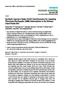
The standard moving and stationary target acquisition and recognition (MSTAR) database [17] The standard moving and stationary target acquisition and recognition (MSTAR) database [17] has 10 SAR targets, which will be discussed in the next section. Instead of putting the MSTAR images 10 SAR targets, which will be discussed the nextimages section.are Instead of putting MSTAR Thehas reasons are that the dimensions of the in MSTAR so large that itthe makes theimages classifier into the SRC directly, some measures should be taken to reduce the dimensions of the MSTAR images. into the SRCtime, directly, some measures should be taken to reduce the dimensions of the MSTAR images.the take too much and simultaneously, the speckle noise in the MSTAR images will influence The reasons are that the dimensions of the MSTAR images are so large that it makes the classifier take The reasons are the dimensions of the the MSTAR images are so large that it makes the classifier take performance thethat classifier; moreover, the raw SAR images notinfluence consistent too much of time, and simultaneously, the dimensions speckle noiseofin the MSTAR imagesare will thewith too much time, and simultaneously, the speckle noise in the MSTAR images will influence the each other, e.g., images of BTR70 are 128 ˆ 128 pixels, 2S1 are 158 ˆ 158 pixels, T62 are 172 ˆ 173 pixels. performance of the classifier; moreover, the dimensions of the raw SAR images are not consistent performance of the classifier; moreover, the dimensions of the raw SAR images are not consistent So it is necessary to reduce the dimensions, and before that, we need to unify the sizes of the images. with each other, e.g., images of BTR70 are 128 × 128 pixels, 2S1 are 158 × 158 pixels, T62 are with each other, e.g., images of BTR70 are 128 × 128 pixels, 2S1 are 158 × 158 pixels, T62 are There a registration in [16] to center training and andbefore test images. theunify images 172 is × 173 pixels. So itmethod is necessary to reduce the the dimensions, that, weThen need to the are 172 × 173 pixels. So it is necessary to reduce the dimensions, and before that, we need to unify the sizes ofinto the the images. a registration method in [16] to center we the do training and test Then cropped sameThere size is according to the “center”. However, not think theimages. method should sizes of the images. There is a registration method in [16] to center the training and test images. Then the images are to cropped into same size according to the However, we do not think the for be adopted here achieve thethe unification. The shadow of“center”. the target in the SAR image is useful the images are cropped into the same size according to the “center”. However, we do not think the method should be adopted here to achieve the unification. The shadow of the target in the SAR image classification, but the method,here however, calculates the “center” according to the intensity of the image, method should be adopted to achieve the unification. The shadow of the target in the SAR image useful for classification, butin thea method, however, calculates the “center” according to the intensity andisisthen it crops the “center” 44 ˆ 44 pixel patch, which barely contains the shadow as seen useful for classification, but the method, however, calculates the “center” according to the intensity in of the and then crops “center”of in a 44shadow × 44 pixelispatch, contains the shadow Figure 1.image, The reason is it that thethe intensity evenwhich lowerbarely than the speckle of the image, and then it crops the “center” inthe a 44 × 44 pixel patch, which barely contains the noise, shadowthus as seen in Figure 1. The reason is that the intensity of the shadow is even lower than the speckle noise, making thein“center” located between theintensity target and speckle center 64 pixel patch as seen Figure 1. The reason is that the of the shadownoise. is evenThe lower than 64 theˆ speckle noise, thus making the “center” located between the target and speckle noise. The center 64 × 64 pixel patch adopted in [10] does not contain enough information the shadow. Therefore, the64center 80 ˆpatch 80 pixel thus making the “center” located between the target of and speckle noise. The center × 64 pixel adopted in [10] does not contain enough information of the shadow. Therefore, the center adopted [10] does not contain enough information theimage, shadow. Therefore,here the because center it patch, whoseincenter is located according to the size of theofraw is adopted 80 × 80 pixel patch, whose center is located according to the size of the raw image, is adopted here 80 × 80 pixel the patch, whose centerand is located according to the size of the raw image, is adopted here contains nearly whole shadow excludes most speckle noise. because it contains nearly the whole shadow and excludes most speckle noise. because it contains nearly the whole shadow and excludes most speckle noise.

Figure 1. The 128 128pixel pixelpatch patch is one one of and thethe other three patches are are Figure 1. The 128 ˆ ×128 of the theBTR70 BTR70raw rawimages, images, and other three patches Figure 1. The 128 × 128 pixel patch is one of the BTR70 raw images, and the other three patches are cropped patches from the 128 × 128 pixel patch. cropped patches from thethe 128 ˆ×128 cropped patches from 128 128pixel pixel patch. patch.

Figure 2. The flow-process diagram of SRC. Figure 2. The flow-process diagram of SRC.

Figure 2. The flow-process diagram of SRC. After the unification of all images, conventional and unconventional feature extraction methods After the unification of all images, conventional and unconventional feature extraction methods are applied extract the features and reduce the dimensions of the cropped images. Then, the feature After the to unification all images, conventional and unconventional methods are applied to extract theoffeatures and reduce the dimensions of the cropped feature images. extraction Then, the feature vectors are inputted into the SRC to achieve the classification. The overall procedure of the are applied to extract the into features the dimensions of the cropped images. Then, the vectors are inputted the and SRCreduce to achieve the classification. The overall procedure of feature the classification is summarized in Figure 2. The two successive steps, cropping the images and extracting vectors are inputted into the SRC to achieve thetwo classification. The overall procedure ofand the extracting classification classification is summarized in Figure 2. The successive steps, cropping the images feature vectors, are applied to both test and training samples to generate the test and training vectors, feature vectors, are applied both test and training samples to generate and training vectors, is summarized in Figure 2. Thetotwo successive steps, cropping the imagesthe andtest extracting feature vectors, respectively. Then, the feature vectors are inputted into the Sparse-Representation module, which respectively. Then, the feature vectors are inputted into the Sparse-Representation module, which areconstructs applied tothe both test and training samples to generate the test and training vectors, respectively. dictionary and solves the sparse coefficients. The dictionary will be achieved by the constructs the dictionary and solves the sparseSparse-Representation coefficients. The dictionary will be achieved by the the Then, the feature module, constructs training vectors,vectors and itare is inputted combinedinto withthe the test vectors to solve the sparsewhich coefficients. The training vectors, and it is combined with the test vectors to solve the sparse coefficients. The dictionary and solves the sparse coefficients. The dictionary will be achieved by the training vectors,

and it is combined with the test vectors to solve 4the 4 sparse coefficients. The dictionary and sparse coefficients are to be utilized to reconstruct the test vectors. Then the reconstructive errors are calculated to infer the identities of the test samples.

Appl. Sci. 2016, 6, 26 Appl. Sci. 2016, 6, 26

5 of 11

dictionary and sparse coefficients are to be utilized to reconstruct the test vectors. Then the reconstructive errors are calculated to infer the identities of the test samples. 4. Experiment Results 4. The Experiment MSTARResults database [17] has 10 SAR targets, which are BMP2, T72, T62, BTR70, BTR60, 2S1, BRDM2,The D7,MSTAR ZIL131 database and ZSU234. The10 images of thesewhich targetsare areBMP2, collected twoBTR70, different depression [17] has SAR targets, T72,atT62, BTR60, 2S1, ˝ ˝ ˝ ˝ angles (15 D7, andZIL131 17 ) over full 0 –360 rangeofofthese aspect view. experimental procedure adopted BRDM2, and aZSU234. The images targets areThe collected at two different depression in this article follows the guideline [18], which statesview. that classifiers using this database are toinbe angles (15° and 17°) over a full 0°–360° range of aspect The experimental procedure adopted trained usingfollows targetsthe at guideline the 17˝ depression tested on using targets atdatabase the 15˝ depression angle. this article [18], whichangle states and that classifiers this are to be trained using targets the at targets the 17°BMP2 depression angle testedvariants on targets at the 15° depression angle. Simultaneously, and T72 haveand different (BMP2-9563, BMP2-9566, BMP2-C21, Simultaneously, targetswhich BMP2 and be T72included have different BMP2-9566, T72-132, T72-812 andthe T72-S7), should in the testvariants set. The(BMP2-9563, training set, however, only T72-132, T72-812 and T72-S7), which should beshould included in the test The training set, hasBMP2-C21, variants BMP2-C21 and T72-132, because the classifier recognize theset. variants not present however, only variants BMP2-C21 and T72-132, because should theset in the training set.has The number of each target available at the the 17˝ classifier training set and recognize the 15˝ test variants not present in the training set. The number of each target available at the 17° training set and depression angles are listed in Table 1. Meanwhile, the optical images of the 10 targets are displayed the 15° 3. test set depression angles are listed in Table 1. Meanwhile, the optical images of the 10 targets in Figure are displayed in Figure 3. Table 1. The number of images of each object at different depression angles. Table 1. The number of images of each object at different depression angles. TargetsBMP2 BMP2 BTR70 BTR70 T72 T72 BTR60 BTR60 2S1 2S1 BRDM2 BRDM2 D7 Targets D7 T62 T62 ZIL131 ZIL131ZSU234 ZSU234 ˝

17°17 15˝ 15°

233233 587 587

233233 196 196

232 232 582 582

256 256 195 195

299 299 274 274

298 298 274

299 299 299 299 274 273

274

274

273

299 299 274

274

299 299 274

274

Figure 3. The optical imagesofofthe the10 10targets. targets. Among Among them, them, the BRDM2, Figure 3. The optical images the T62 T62and andT72 T72are aretanks. tanks.The The BRDM2, BMP2, BTR60 and BTR70 are armored personnel carriers. The 2S1 is a rocket launcher, the D7D7 is is a a BMP2, BTR60 and BTR70 are armored personnel carriers. The 2S1 is a rocket launcher, the bulldozer, ZIL131 a truck andthe theZSU234 ZSU234isisan anAir Air Defense Defense Unit. Unit. bulldozer, thethe ZIL131 is is a truck and Table 2. The recognition rates of the cropped images using SRC. Table 2. The recognition rates of the cropped images using SRC.

Patch

44 × 44 Pixel

64 × 64 Pixel

80 × 80 Pixel

Patch

44 ˆ 44 Pixel

64 ˆ 64 Pixel

80 ˆ 80 Pixel

Accuracy

34.1%

64.3%

75.1%

Accuracy

34.1%

64.3%

75.1%

The preprocessing of the SAR images was discussed in last section. Table 2 shows the recognition rates the three cropped images under SRC. From the table, 80 × 80Table pixel 2patch indeed contains Theofpreprocessing of the SAR images was discussed in lastthe section. shows the recognition more effective information than the other patches. After unifying the sizes of the images, the rates of the three cropped images under SRC. From the table, the 80 ˆ 80 pixel patch indeed unconventional methods, down-sample and Principal Component Analysis (PCA), are utilized to contains more effective information than the other patches. After unifying the sizes of the images, extract the features of the cropped images. The down-sample is achieved by bilinear interpolation the unconventional methods, down-sample and Principal Component Analysis (PCA), are utilized to here, and the output pixel value is a weighted average of pixels in the nearest two-by-two extract the features of the cropped images. The down-sample is achieved by bilinear interpolation here, neighborhood. In comparison with the down-sample, the dimensions of the feature vector extracted and the output pixel value is a weighted average of pixels in the nearest two-by-two neighborhood. by PCA are the same as the former. Meanwhile, the conventional features, baseline features [19], are In comparison the down-sample, the dimensions of the feature vector extracted by PCA are the adopted herewith to make a comparison with the unconventional features. In order to achieve excellent same as the former. Meanwhile, the conventional features, baseline features [19], are adopted here performance of SVM [20], the multiclass classifier, based on the one-against-one approach, adopts to make a comparison with the unconventional In order to achieve excellentbecause performance the feature normalization method if there is features. no additional stress. Simultaneously, the of SVM [20], the multiclass classifier, based on the one-against-one approach, adopts the feature 5 normalization method if there is no additional stress. Simultaneously, because the different features are

Appl. Sci. 2016, 6, 26 Appl. Sci. 2016, 6, 26

6 of 11

different features are employed here, SVM uses a linear method to deal with down-sampling features employed here, SVM uses a linear method to deal with down-sampling features and baseline features, and baseline features, and uses the Gaussian kernel method to process PCA features. and uses the Gaussian kernel method to process PCA features. 4.1. Recognition Classifiers 4.1. Recognition Accuracy Accuracy of of Two Two Classifiers Owing to dimensions of the features, the comparison under theunder two classifiers Owing tothe thefinite finite dimensions of baseline the baseline features, the comparison the two between the conventional features features and the and unconventional features is listed firstly. Then, the classifiers between the conventional the unconventional features is listed firstly. Then, dimensions of the unconventional features are enlarged to verify the performances of the two the dimensions of the unconventional features are enlarged to verify the performances of the two classifiers further. further. classifiers Features 4.1.1. Comparison between Conventional Features and Unconventional Features According to [19,21] and the down-sampling method used here, the dimensions of the baseline features adopted adopted are are sizes sizes of of 16, 16, 36 36 and and 81, 81, which which are are represented representedby byDM DM11,, DM DM22 and DM33,, respectively. features respectively. In order ordertotocompare compare them to the conventional features, the unconventional feature them to the conventional features, the unconventional feature extractionextraction methods methodsthe reduce the dimensions of the cropped image to the size sameassize the former. Considering the reduce dimensions of the cropped image to the same theasformer. Considering the big big differences within the baseline features, thedoes SVM feature normalization differences within the baseline features, the SVM notdoes adoptnot theadopt featurethe normalization method in method in this experiment. this experiment.

Figure 4. 4. The The recognition recognitionaccuracy accuracyofofthe the two classifiers under different feature spaces; (a) (b) andrefer (b) Figure two classifiers under different feature spaces; (a) and 1, DM2 and 3 stand DM refer to the recognition accuracy achieved by SRC and SVM, respectively. DM 1 2 3 to the recognition accuracy achieved by SRC and SVM, respectively. DM , DM and DM stand for the for the dimensions of feature spaces adopted here that have 16, 81, 36 and 81, respectively. dimensions of feature spaces adopted here that have sizes of sizes 16, 36ofand respectively.

Figure 4 shows the recognition accuracy of the two classifiers under different feature spaces. Figure 4 shows the recognition accuracy of the two classifiers under different feature spaces. Figure 4a plots the recognition accuracy under different feature spaces of SRC, and Figure 4b plots Figure 4a plots the recognition accuracy under different feature spaces of SRC, and Figure 4b plots that that of SVM. Compared with the unconventional features, the recognition rates of the two classifiers of SVM. Compared with the unconventional features, the recognition rates of the two classifiers under under baseline features are nearly highest. So in the low-dimensional feature spaces, baseline features baseline features are nearly highest. So in the low-dimensional feature spaces, baseline features are are better for describing the targets. Simultaneously, the highest recognition rates of SRC and SVM better for describing the targets. Simultaneously, the highest recognition rates of SRC and SVM are are almost identical, but SRC implies that the precise choice of feature space is no longer critical [14]. almost identical, but SRC implies that the precise choice of feature space is no longer critical [14]. That is That is to say that when the dimensions of the feature space surpasses a certain threshold, to say that when the dimensions of the feature space surpasses a certain threshold, unconventional unconventional features perform just as well as conventional features towards SRC. From Figure 4a, features perform just as well as conventional features towards SRC. From Figure 4a, the dimension the dimension threshold in this experiment is near 80. threshold in this experiment is near 80. 4.1.2. Recognition Unconventional Feature Feature Spaces Spaces 4.1.2. Recognition Accuracy Accuracy under under Unconventional The recognition recognitionrates ratesofofthe the two classifiers under different unconventional feature are The two classifiers under different unconventional feature spacesspaces are listed 1, Down-sample 2 and Down-sample 3 stand for reducing the listed in Table 3. Down-sample 1 2 3 in Table 3. Down-sample , Down-sample and Down-sample stand for reducing the dimensions 1, dimensions of the cropped image by down-sample to sizes of 100, 400respectively. and 1600, respectively. 2 and of the cropped image by down-sample to sizes of 100, 400 and 1600, PCA1 , PCAPCA 2 4 PCA4 and PCA represent that the dimensions of the cropped image are reduced PCA to of PCA represent that the dimensions of the cropped image are reduced by PCA by to sizes of sizes 25, 100 3 25, 100 and 400. Additionally, PCA refers to reducing the dimensions to the extent where the and 400. Additionally, PCA3 refers to reducing the dimensions to the extent where the accumulative accumulativerate contribution rate approximately equals 80%, because the empirical valuethe guarantees contribution approximately equals 80%, because the empirical value guarantees reduced the reduced dimensions will cover all the primary information. In this experiment, PCA3 stands for 6

Appl. Sci. 2016, 6, 26 Appl. Sci. 2016, 6, 26

7 of 11

3 stands for reducing the dimensions cover all to thea primary information. In3,this experiment, PCA reducing thewill dimensions size of 125. From Table SRC achieves the highest recognition rates in dimensions to a size of 125. From Table 3, SRC achieves the highest recognition rates bothSVM feature both feature spaces. The recognition rates of SRC are 3.03%, 4.18% and 4.46% betterinthan in 2, 2 3 2 spaces. The recognition rates of SRC are 3.03%,Figure 4.18% and 4.46% better SVMthe in tendency Down-sample Down-sample , PCA and PCA , respectively. 5 is plotted here than to study of the 3 2 PCA and PCA , respectively. Figure 5 is plotted here to study the tendency of the recognition accuracy. recognition accuracy.

Table 3. Table 3. The The recognition recognition accuracy accuracy under under different different unconventional unconventional feature feature spaces. spaces. 3 1 4 3 1 3 Down-Sample 1 PCA 4 PCAPCA 3 PCAPCA 2PCA2PCAPCA 1 Features Down-Sample22 Down-Sample Down-Sample Features Down-Sample Down-Sample

SVM SVM SRCSRC

86.79% 86.79% 72.93% 72.93%

86.73% 86.73% 89.76% 89.76%

84.39% 71.84%71.84% 74.71% 74.40% 59.19% 84.39% 74.71% 74.40% 59.19% 81.83% 70.34% 78.89% 78.86% 54.04% 81.83% 70.34% 78.89% 78.86% 54.04%

Figure 5. 5. The The recognition recognition rates rates under under different different unconventional unconventional feature feature spaces; spaces; (a,b) (a,b) are are two two forms forms of of Figure 3 3 the dimensions of the the cropped cropped image image to to aa size size the recognition recognition rates. rates. Down-sample Down-sample refers the refers to to reducing reducing the dimensions of Down-sample11,, PCA PCA44,, PCA PCA33,, PCA PCA22 and and PCA PCA11 of 1600 1600 by bydown-sample. down-sample. Similarly, Similarly,Down-sample Down-sample22,, Down-sample of stand for for sizes sizes of of 400, 400, 100, 100, 400, 400, 125, 125, 100 100 and and 25, 25, respectively. respectively. stand

Figure 5 shows the recognition rates under different unconventional feature spaces. Figure 5a,b Figure 5 shows the recognition rates under different unconventional feature spaces. Figure 5a,b are two forms of the recognition rates. Figure 5a is a column diagram, and Figure 5b is a line chart. are two forms of the recognition rates. Figure 5a is a column diagram, and Figure 5b is a line chart. The two feature spaces are divided in Figure 5b. Meanwhile, different colors are adopted here to The two feature spaces are divided in Figure 5b. Meanwhile, different colors are adopted here to 3 and represent different classifiers. Obviously, SRC is indeed superior to SVM in Down-sample2, PCA 2 , PCA 3 represent different classifiers. Obviously, SRC is indeed superior to SVM in Down-sample PCA2. However, with increments of decreases of the dimensions, the performances of both classifiers and PCA2 . However, with increments of decreases of the dimensions, the performances of both tend to descend. The reason is that speckle noise will be added into the data with increasing classifiers tend to descend. The reason is that speckle noise will be added into the data with increasing dimensions [10]. Simultaneously, when the dimensions of the data decrease, the data is too small to dimensions [10]. Simultaneously, when the dimensions of the data decrease, the data is too small cover all the primary information. The performance of SRC descends a little faster than SVM. to cover all the primary information. The performance of SRC descends a little faster than SVM. Additionally, the performances of both classifiers in the down-sampling spaces are better than that Additionally, the performances of both classifiers in the down-sampling spaces are better than that in the spaces of PCA. That is to say, down-sample contains more effective information than PCA in in the spaces of PCA. That is to say, down-sample contains more effective information than PCA in this experiment. this experiment. 4.2. Recognition Accuracy under under Incomplete Incomplete Training Training Samples Samples 4.2. Recognition Accuracy In the the last last subsection, subsection, all all samples samples at at the the 17 17° depression angle angle over over aa full full 00°–360° range of of the the ˝ depression ˝ –360˝ range In aspect view vieware areused used to train the classifiers. the real-world tasks, data cannot cover all aspect to train the classifiers. In theIn real-world tasks, the data the cannot cover all conditions conditions of the targets. In this experiment, a certain percentage of samples at the 17° depression ˝ of the targets. In this experiment, a certain percentage of samples at the 17 depression angle are angle are randomly to the construct theset, training all theatsamples the 15° depression randomly selected toselected construct training and allset, theand samples the 15˝ at depression angle are 3 angle are tested. The feature space, PCA , is adopted here, which is to say that the dimensions of 3 tested. The feature space, PCA , is adopted here, which is to say that the dimensions of samples samples are reduced to the extent where the accumulative contribution rate is approximately equal are reduced to the extent where the accumulative contribution rate is approximately equal to 80% to 80%classification. before classification. before Figure under different percentages of training samples. The Figure 66 shows shows the therecognition recognitionrates rates under different percentages of training samples. recognition rates of the two classifiers rise with the increasing percentage of the training samples. In The recognition rates of the two classifiers rise with the increasing percentage of the training samples. other words, both the classifiers are sensitive to the number of samples in the training set.

7

Appl. Sci. 2016, 6, 26

8 of 11

In other words, both the classifiers are sensitive to the number of samples in the training set. Appl. Sci. 2016, 6, 26 Additionally, with the decreasing percentage of the training samples, the recognition accuracy of the decreasing percentage of the training samples, the recognition accuracy of SVM descends Additionally, faster thanwith that of SRC, so SRC is more robust than SVM in this experiment. SVM descends faster than that of SRC, so SRC is more robust than SVM in this experiment.

Figure 6. The recognition rates under different percentages of training samples. The horizontal

Figure 6. The coordinate recognition under different percentages of training stands rates for the percentage of training samples, and the vertical coordinatesamples. represents theThe horizontal recognition accuracy. coordinate stands for the percentage of training samples, and the vertical coordinate represents the recognition 4.3. accuracy. Recognition Rate of Each Object The average recognition rates of the classifiers are an objective evaluation index of their Simultaneously, further information is found by listing the recognition rate of each 4.3. Recognition performance. Rate of Each Object target here. The confusion matrix is a good reflection of the recognition rate of each object. However, not all confusion matrices in the of the two classifiers are needed to be listed here, index of their The average recognition rates offeature the spaces classifiers are an objective evaluation because the information they try to convey is similar. Table 4 lists the 10-class target confusion performance. Simultaneously, further information is found by listing the recognition rate of each target matrices of the two classifiers under the feature spaces of Down-sample2, PCA4 and PCA2, which are here. The confusion matrix explained above. is a good reflection of the recognition rate of each object. However, not all common that the recognition rates of BMP2 and T72 are very low. The reason is that confusion matricesFirstly, in theit isfeature spaces of the two classifiers are needed to be listed here, because the there are many variants of the two targets, which are not included in the training set, in the test set. information they to convey is similar. Table 4 lists the 10-class confusion of the two So try the variant has a more important influence in classification than target the depression angle inmatrices this 2 , PCA 2 , which experiment for only 2° difference in the depression angle. With4anand increasing in depression classifiers under the feature spaces of Down-sample PCAdifference are explained above. angle, the recognition rates indeed descend rapidly [9]. Then, the recognition rates of BRDM2 are Firstly, it is common the spaces recognition ratestheof BMP2 and T72is too aresmall very low. The reason is obviously low inthat the feature of PCA, because dimensionality of PCA to contain all the primary information. To illustrate it, Figure 7 is plotted. The figure shows the average that there are many variants of the two targets, which are not included in the training set, in the recognition rate and the recognition rate per target of SRC under different PCA feature spaces. PCA2 test set. So theand variant has a more important influence in classification than the depression angle PCA4 are described above. PCA5 and PCA6 refer to reducing the dimensions of the cropped image in this experiment only 2˝ difference in the depression angle. With an increasing to 900 for and 1600 by PCA, respectively. From Figure 7, the recognition rate of BRDM2 indeed rises with difference in the increasing dimensions of PCA. Similarly, BTR70 enjoys the same trend, which is more moderate depression angle, the recognition rates indeed descend rapidly [9]. Then, the recognition rates of than BRDM2. Contrarily, the recognition rates of other targets tend to descend with the increasing BRDM2 are obviously inshape the of feature spaces of PCA, because the dimensionality dimensions,low and the the average recognition rate in Figure 7 is a response to that. Therefore, of PCA is too it is not wise to improve the recognition accuracy of one object, sacrificing the whole performance. small to contain all the primary information. To illustrate it, Figure 7 is plotted. The figure shows Last but not least, the classifiers both tend to classify other targets into 2S1 incorrectly, which is the average recognition rate and the recognition rate per target of SRC under different PCA feature mainly caused by its structures. The structures, such as the barrel and upper surface, make it similar 4 areT62) 6 refer to tanks and armored personnel (BMP2, BTR60, and BRDM2). spaces. PCA2 and PCA(T72, described above. PCA5carriers and PCA to BTR70 reducing the dimensions of the Simultaneously, it is no wonder that the classifiers classify 2S1 into other targets. cropped image to 900 and 1600 by PCA, respectively. From Figure 7, the recognition rate of BRDM2 indeed rises with the increasing dimensions of PCA. Similarly, BTR70 enjoys the same trend, which is 8 more moderate than BRDM2. Contrarily, the recognition rates of other targets tend to descend with the increasing dimensions, and the shape of the average recognition rate in Figure 7 is a response to that. Therefore, it is not wise to improve the recognition accuracy of one object, sacrificing the whole performance. Last but not least, the classifiers both tend to classify other targets into 2S1 incorrectly, which is mainly caused by its structures. The structures, such as the barrel and upper surface, make it similar to tanks (T72, T62) and armored personnel carriers (BMP2, BTR60, BTR70 and BRDM2). Simultaneously, it is no wonder that the classifiers classify 2S1 into other targets.

Appl. Sci. 2016, 6, 26

9 of 11

Table 4. The 10-class target confusion matrices of two classifiers under different feature spaces. Features

a

SVM

b

c

Targets BMP2 BMP2 83.6 BTR70 2.0 T72 9.6 BTR60 1.0 2S1 0.4 BRDM2 1.1 D7 0.0 T62 0.4 ZIL131 0.0 ZSU234 0.0 BMP2 71.7 BTR70 1.5 T72 12.2 BTR60 1.0 2S1 1.8 BRDM2 4.7 D7 0.0 T62 1.5 ZIL131 0.4 ZSU234 0.7 BMP2 75.6 BTR70 2.0 T72 11.3 BTR60 2.6 2S1 3.6 BRDM2 2.2 D7 0.0 T62 0.7 ZIL131 0.4 ZSU234 2.6

BTR70 1.5 93.9 0.7 1.5 0.0 2.2 0.0 0.0 0.0 0.0 8.2 91.3 6.5 5.6 8.0 1.5 0.0 2.9 0.0 0.4 5.8 86.7 4.1 5.6 4.7 4.4 0.0 1.1 0.4 0.0

T72 8.5 0.0 73.0 0.0 1.5 0.4 0.0 0.7 0.0 0.0 8.3 0.0 49.0 1.0 4.4 1.5 0.4 4.4 0.4 1.1 9.4 2.6 62.0 1.0 7.3 5.8 0.0 1.8 1.5 0.0

BTR60 2.0 0.0 0.0 95.4 1.1 4.4 0.0 0.0 0.0 0.0 4.3 4.6 2.1 85.1 1.5 3.6 0.4 0.4 1.1 0.4 3.1 3.1 0.7 84.6 1.5 5.5 0.7 0.4 0.0 2.6

2S1 4.1 4.1 5.5 0.0 92.3 3.3 0.4 3.3 0.4 0.0 2.6 1.5 13.4 2.6 74.8 3.6 0.0 12.8 10.6 0.4 2.6 5.6 11.0 1.0 70.4 8.4 0.4 13.2 1.8 0.0

BRDM2 D7 0.0 0.0 0.0 0.0 0.0 0.0 0.5 0.0 0.7 0.0 85.0 0.0 0.4 97.4 0.0 0.7 0.0 0.4 0.0 4.4 2.6 0.2 1.0 0.0 2.7 0.7 2.6 0.0 0.4 0.0 73.7 0.0 1.5 89.8 1.8 1.5 0.0 1.5 0.7 9.5 2.7 0.0 0.0 0.0 4.1 0.3 3.6 0.0 3.6 0.0 63.9 0.0 0.0 96.0 7.0 0.7 1.8 0.7 7.3 6.9

T62 0.2 0.0 10.3 0.5 3.3 0.0 0.0 79.5 2.2 0.4 0.9 0.0 7.9 0.5 4.7 4.7 1.5 63.7 5.1 6.6 0.3 0.0 4.1 1.0 4.7 2.9 0.4 61.9 4.0 5.1

ZIL131 0.0 0.0 0.9 0.0 0.7 3.3 0.0 9.5 96.4 1.1 0.3 0.0 5.2 0.0 3.3 4.0 1.1 6.2 79.2 5.1 0.0 0.0 2.2 0.0 3.6 5.5 0.7 8.4 89.1 2.9

ZSU234 0.0 0.0 0.0 1.0 0.0 0.4 1.8 5.9 0.7 94.2 1.0 0.0 0.3 1.5 1.1 2.6 5.5 4.8 1.8 75.2 0.5 0.0 0.0 0.5 0.4 1.5 1.8 4.8 0.4 72.6

Features

a

SRC

b

c

Targets BMP2 BMP2 79.4 BTR70 0.0 T72 8.1 BTR60 0.0 2S1 0.4 BRDM2 0.4 D7 0.0 T62 0.7 ZIL131 0.0 ZSU234 0.0 BMP2 46.2 BTR70 0.0 T72 0.0 BTR60 0.0 2S1 0.0 BRDM2 0.0 D7 0.0 T62 0.0 ZIL131 0.4 ZSU234 0.0 BMP2 71.6 BTR70 0.0 T72 0.3 BTR60 0.0 2S1 0.0 BRDM2 0.0 D7 0.0 T62 0.0 ZIL131 0.0 ZSU234 0.0

BTR70 4.1 98.5 5.2 0.0 0.0 2.9 0.0 0.0 0.0 0.0 1.7 89.3 1.5 0.0 0.0 0.0 0.0 0.0 0.0 0.0 2.9 86.2 2.1 1.0 0.0 0.4 0.0 0.0 0.0 0.0

T72 10.2 0.5 77.8 0.0 1.1 5.5 0.7 0.7 0.0 0.0 0.9 0.0 37.5 0.0 0.0 0.0 0.0 0.4 0.0 0.0 1.5 0.5 50.0 1.0 0.7 0.0 0.0 1.1 0.0 0.0

BTR60 3.6 1.0 7.6 100.0 0.7 3.3 0.0 1.1 2.2 0.4 0.3 0.0 0.2 91.3 0.0 0.4 0.0 0.4 0.4 0.0 0.5 1.5 1.0 95.4 0.0 2.9 0.4 0.4 0.0 0.0

2S1 0.3 0.0 0.0 0.0 95.6 1.1 0.0 0.0 0.4 0.4 7.3 2.6 10.1 2.1 89.8 4.0 0.4 3.3 2.6 0.4 6.0 4.6 5.7 0.0 93.8 2.6 0.0 1.8 0.7 0.0

BRDM2 0.7 0.0 1.0 0.0 2.2 86.5 0.0 0.7 0.0 0.0 0.3 0.0 0.0 0.0 0.0 67.2 0.0 0.0 0.0 0.0 0.7 0.0 0.2 0.5 0.0 61.7 0.0 0.0 0.0 0.0

D7 0.5 0.0 0.0 0.0 0.0 0.4 99.3 0.4 0.0 0.7 16.0 2.0 14.9 4.1 3.3 7.3 98.5 7.3 7.7 7.3 2.7 1.5 6.9 1.0 0.4 5.1 98.5 3.3 0.7 2.2

T62 0.3 0.0 0.2 0.0 0.0 0.0 0.0 95.6 0.4 0.0 10.6 3.6 17.0 0.5 3.3 7.3 0.7 83.2 2.6 1.5 5.8 1.0 22.0 1.0 3.3 7.3 0.0 86.4 0.7 2.2

ZIL131 0.0 0.0 0.0 0.0 0.0 0.0 0.0 0.0 97.1 0.0 4.1 0.5 7.6 0.0 0.7 6.6 0.4 3.3 85.8 0.0 1.2 2.0 4.8 0.0 0.4 11.7 1.1 5.5 97.4 0.4

ZSU234 0.9 0.0 0.2 0.0 0.0 0.0 0.0 0.7 0.0 98.5 12.6 2.0 11.2 2.1 2.9 7.3 0.0 2.2 0.7 90.9 7.2 2.6 7.0 0.0 1.5 8.4 0.0 1.5 0.4 95.3

*a, b, c refer to the confusion matrices generated under Down-sample2 , PCA4 and PCA2 , respectively. Down-sample2 refers to reducing the dimensions of the cropped image to a size of 400 by down-sample; similarly, PCA4 and PCA2 stand for sizes of 400 and 100 by PCA, respectively.

Appl. Sci. 2016, 6, 26 Appl. Sci. 2016, 6, 26

10 of 11

Figure 7. 7. The PCA feature feature spaces; spaces; PCA PCA22 refers reducing the the Figure The recognition recognition rates rates of of SRC SRC under under PCA refers to to reducing 4, PCA55 and PCA66 stand for 4 dimensions of the cropped image to a size of 100 by PCA; similarly, PCA dimensions of the cropped image to a size of 100 by PCA; similarly, PCA , PCA and PCA stand for sizes of of 400, 400, 900 900 and and 1600, 1600, respectively. respectively. sizes

5. Conclusions 5. Conclusions In this sparse representation-based representation-based classification classification has has been been applied applied to In this paper, paper, sparse to the the 10-class 10-class MSTAR MSTAR data set. preprocessing method of the MSTAR images is introduced to unify sizes the images, data set.AA preprocessing method of the MSTAR images is introduced to the unify theofsizes of the reduce the complexity and improve the performance of the classifiers. Then, the identity of identity the test images, reduce the complexity and improve the performance of the classifiers. Then, the sample is sample inferredisby the framework of SRC. of Compared with SVM, good of the test inferred by the framework SRC. Compared with SRC SVM,also SRCachieves also achieves performance of recognition accuracy, and when the dimensions of the feature space surpass a certain good performance of recognition accuracy, and when the dimensions of the feature space surpass a threshold, the performances of the under conventional certain threshold, the performances of classifiers the classifiers under conventionaland andunconventional unconventional features features converge. Additionally, Additionally,the therecognition recognitionrate rateofofeach eachtarget targetalso alsohas hasbeen beendiscussed. discussed. The performance converge. The performance is is badly influenced byvariation the variation of theconfigurations target configurations and articulations, thedepression different badly influenced by the of the target and articulations, the different depression the the sensor andangles the aspect of which the targets, is an open problem called angles in theangles sensorinand aspect of theangles targets, is an which open problem called over-fitting. over-fitting. Simultaneously, the wrong ofclassification of the BRDM2 specific and targets and further. 2S1 is Simultaneously, the wrong classification the specific targets 2S1 BRDM2 is discussed discussed further. The main reason is that the feature extraction methods cannot describe the targets The main reason is that the feature extraction methods cannot describe the targets effectively. effectively. Taking the minor flaws into consideration, on one hand, the future work will focus on improving Taking theofminor intowords, consideration, on one framework hand, the future work will be focus on improving the robustness SRC. flaws In other a more efficient of SRC should explored. On the the robustness of SRC. In other words, a more efficient framework of SRC should be explored. On other hand, we expect to find more effective features to describe the targets. Although baseline features the other hand, we expect to find more effective features to describe the targets. Although baseline are studied here, conventional features need to be enriched to describe targets more effectively and so features are studied here, conventional features need to be enriched to describe targets more do the unconventional features. effectively and so do the unconventional features. Acknowledgments: This work is partially supported by the National Natural Science Foundation of China under Acknowledgments: This work is partially supported by the National Natural Science Foundation of China Grant 61372163 and 61240058. under Grant 61372163 and 61240058. Author Contributions: Haibo Song performed the simulations and algorithm analysis, and contributed to a main Author Contributions: Haibo Song performed the simulations and algorithm analysis, and contributed a main part of manuscript writing. Kefeng Ji contributed in conceiving and the structure of the manuscript. Alltoauthors contributed to the writing the paper. part of manuscript writing.ofKefeng Ji contributed in conceiving and the structure of the manuscript. All authors contributed the writing of the paper. Conflicts of to Interest: The authors declare no conflict of interest.

Conflicts of Interest: The authors declare no conflict of interest.

References

References 1. Thiagarajan, J.; Ramamurthy, K.; Knee, P.P.; Spanias, A.; Berisha, V. Sparse representation for automatic target classification in SAR images. In P. Proceedings Communications, Control and Signal 1. Thiagarajan, J.; Ramamurthy, K.; Knee, P.; Spanias,ofA.; Berisha, V. Sparse representation forProcessing automatic (ISCCSP), 2010 4th International Symposium on, Limassol, Cyprus, 3–5 March 2010. target classification in SAR images. In Proceedings of Communications, Control and Signal Processing 2. Owirka, G.J.; S.M.; Novak, L.M. Template-based ATR performance (ISCCSP), 2010Verbout, 4th International Symposium on, Limassol, SAR Cyprus, 3–5 March 2010.using different image enhancement techniques. Proc. SPIE 1999, 3721, 302–319. 2. Owirka, G.J.; Verbout, S.M.; Novak, L.M. Template-based SAR ATR performance using different image enhancement techniques. Proc. SPIE 1999, 3721, 302–319.

11

Appl. Sci. 2016, 6, 26

3. 4.

5. 6.

7.

8.

9. 10. 11.

12. 13.

14. 15.

16. 17. 18.

19.

20. 21.

11 of 11

Patnaik, R.; Casasent, D.P. MSTAR object classification and confuser and clutter rejection using minace filters. In Proceedings of Automatic Target Recognition XVI, Orlando, FL, USA, 17 April 2006. Marinelli, M.P.; Kaplan, L.M.; Nasrabadi, N.M. SAR ATR using a modified learning vector quantization algorithm. In Proceedings of the SPIE Algorithms for Synthetic Aperture Radar Imagery VI, Orlando, FL, USA, 5 April 1999. Yuan, C.; Casasent, D. A new SVM for distorted SAR object classification. In Proceedings of the SPIE Conference on Optical Pattern Recognition XVI, Orlando, FL, USA, 28 March 2005. Huang, J.B.; Yang, M.H. Fast sparse representation with prototype. In Proceedings of the IEEE Computer Society Conference on Computer Vision and Pattern Recognition (CVPR 2010), San Francisco, CA, USA, 13–18 June 2010; pp. 3618–3625. Shin, Y.; Lee, S.; Woo, S.; Lee, H. Performance increase by using an EEG sparse representation based classification method. In Proceedings of the IEEE International Conference on Consumer Electronics, Las Vegas, NV, USA, 2013; pp. 201–203. Huang, X.; Wang, P.; Zhang, B.; Qiao, H. SAR target recognition using block-sparse representation. In Proceedings of the International Conference on Mechatronic Sciences, Electric Engineering and Computer, Shengyang, China, 20–22 December 2013; pp. 1332–1336. Dong, G.; Wang, N.; Kuang, G. Sparse representation of monogenic signal: With application to target recognition in SAR images. IEEE Signal Process. Lett. 2014, 21, 952–956. Xing, X.; Ji, K.; Zou, H.; Sun, J. SAR vehicle recognition based on sparse representation along with aspect angle. Sci. World J. 2014, 2014. [CrossRef] [PubMed] Pati, Y.C.; Rezaiifar, R.; Krishnaprasad, P.S. Orthogonal matching pursuit: Recursive function approximation with applications to wavelet decomposition. In Proceedings of the Conference Record of The Twenty-Seventh Asilomar Conference on Signals, Systems, and Computers, Pacific Grove, CA, USA, 1–3 November 1993; pp. 40–44. Chen, S.; Billings, S.; Luo, W. Orthogonal least squares methods and their application to non-linear system identification. Int. J. Control 1989, 50, 1873–1896. [CrossRef] Candes, E.; Romberg, J. l1 -magic: Recovery of sparse signals via convex programming. California Institute of Technology. 2005. Available online: http://thesis-text-naim-mansour.googlecode.com/svn/trunk/Thesis Text/Thesis%20backup/Literatuur/Optimization%20techniques/l1magic.pdf (accessed on 10 December 2014). Wright, J.; Yang, A.Y.; Ganesh, A.; Sastry, S.S.; Ma, Y. Robust face recognition via sparse representation. IEEE Trans. Pattern Anal. Mach. Intell. 2009, 31, 210–227. [CrossRef] [PubMed] Patnaik, R.; Casasent, D.P. SAR classification and confuser and clutter rejection tests on MSTAR 10-class data using minace filters. In Proceedings of the Optical Pattern Recognition XVIII, (SPIE 6574, 657402), Orlando, FL, USA, 9 April 2007. Yuan, C.; Casasent, D. MSTAR 10-class classification and confuser and clutter rejection using SVRDM. In Proceedings of the Optical Pattern Recognition XVII, (SPIE 6245, 624501), Orlando, FL, USA, 17 April 2006. Moving and Stationary Target Acquisition and Recognition (MSTAR) Public Release Data. Available online: https://www.sdms.afrl.af.mil/datasets/matar/ (accessed on 24 Augest 2015 ). Ross, T.; Worrell, S.; Velten, V.; Mossing, J.; Bryant, M. Stardard SAR ATR evaluation experiments using the MSTAR public release data set. In Proceedings of the SPIE on Algorithms for SAR, Orlando, FL, USA, 13 April 1998; pp. 566–573. El-Darymli, K.; Mcguire, P.; Gill, E.; Power, D.; Moloney, C. Characterization and statistical modeling of phase in single-channel synthetic aperture radar imagery. IEEE Trans. Aerospace Electron. Syst. 2015, 51, 2071–2092. [CrossRef] Chang, C.; Lin, C. LIBSVM: A library for support vector machines. ACM Trans. Intell. Syst. Technol. 2011, 2, 389–396. [CrossRef] Mathworks. Regionprops. Available online: http://tinyurl.com/k58dlqf (accessed on 5 December 2015). © 2016 by the authors; licensee MDPI, Basel, Switzerland. This article is an open access article distributed under the terms and conditions of the Creative Commons by Attribution (CC-BY) license (http://creativecommons.org/licenses/by/4.0/).