advances were all based on this first flight at Kitty Hawk by the American Brothers .... Gavin Walker, Jonathan Friedman, and Rob Aberg(2007), âConfiguration ...
IOSR Journal of Electrical and Electronics Engineering (IOSR-JEEE) e-ISSN: 2278-1676,p-ISSN: 2320-3331, Volume 7, Issue 1 (Jul. - Aug. 2013), PP 28-34 www.iosrjournals.org
Aircraft Takeoff Simulation with MATLAB „Er Naser.F.AB.Elmajdub, „Dr. A. K. Bharadwaj Associate prof., Er. Surya Prakash „Sam Higginbottom Institute of Agriculture, Technology and Science Allahabad India’
Abstract: There are three primary ways for an aircraft to change its orientation relative to the passing air. Pitch (movement of the nose up or down, rotation around the transversal axis), Roll (rotation around the longitudinal axis, that is, the axis which runs along the length of the aircraft) and Yaw (movement of the nose to left or right, rotation about the vertical axis). In straight climbing flight, lift is less than weight. At first, this seems incorrect because if an aircraft is climbing it seems lift must exceed weight. When an aircraft is climbing at constant speed it is its thrust that enables it to climb and gain extra potential energy. Lift acts perpendicular to the vector representing the velocity of the aircraft relative to the atmosphere, so lift is unable to alter the aircraft's potential energy or kinetic energy. This can be seen by considering an aerobatic aircraft in straight vertical flight - one that is climbing straight upwards (or descending straight downwards). Vertical flight requires no lift! When flying straight upwards the aircraft can reach zero airspeed before falling earthwards - the wing is generating no lift and so does not stall. In straight, climbing flight at constant airspeed, thrust exceeds drag. In straight descending flight, lift is less than weight. In addition, if the aircraft is not accelerating, thrust is less than drag. In turning flight, lift exceeds weight and produces a load factor greater than one, determined by the aircraft's angle of bank Take off is the stage from the application of take off power until an altitude of 35 feet above the runway elevation. This includes the substages: takeoff and rejected takeoff. The initial climb is the stage from the end of the takeoff to the first prescribed power reduction or when the aircraft is 1,000 feet above the runway elevation, whichever is first.
I.
Introduction
History of Flight German engineer, Otto Lilienthal, studied aerodynamics and worked to design a glider that would fly. He was the first person to design a glider that could fly a person and was able to fly long distances. He was fascinated by the idea of flight. Based on his studies of birds and how they fly, he wrote a book on aerodynamics that was published in 1889 and this text was used by the Wright Brothers as the basis for their designs. After more than 2500 flights, he was killed when he lost control because of a sudden strong wind and crashed into the ground.
The first heavier-than-air flight The first heavier-than-air flight traveled one hundred twenty feet in twelve seconds. The two brothers took turns during the test flights. It was Orville's turn to test the plane, so he is the brother that is credited with the first flight. Humankind was now able to fly! During the next century, many new airplanes and engines were developed to help transport people, luggage, cargo, military personnel and weapons. The 20th century's advances were all based on this first flight at Kitty Hawk by the American Brothers from Ohio.
II.
Objectives
The Ultimate Goal of all such decision is to minimizes the fault required or to maximize the desire benefitEngineering application of optimization for design aircraft and aerospace structure for minimum weight www.iosrjournals.org
28 | Page
Aircraft Takeoff Simulation with MATLAB with Maximum force.Control system must provide safe operation of people in the aircraft, alarms, safety constraint control, emergency system and environmental protection.To comparison instruments of aircraft with the ground Electronics instrument and to reach into possibility replacement to each other.To study of the important theoretical approaches to the optimal control system design includes calculus of variation, maximum/minimum principle, dynamic programming.To find trajectories that maximize or minimize a given functional optimal control problems.To transform classical results into modern optimal control frame work through plant equation constraint, the concepts and methods are almost similar to those employed in maximum and minimum theory of deferential calculus. Visualize airplanetakeoff and chase airplane with the virtual reality animation object. This illustrates how we can use the Aero.VirtualRealityAnimation object to set up a virtual reality animation based on the asttkoff.wrl file. The scene simulates an airplanetakeoff. Create the Animation Object This code creates an instance of the Aero.VirtualRealityAnimation object. h = Aero.VirtualRealityAnimation; Set the Animation Object Properties This code sets the number of frames per second and the seconds of animation data per second time scaling. 'FramesPerSecond' controls the rate at which frames are displayed in the figure window. 'TimeScaling' is the seconds of animation data per second time scaling. The 'TimeScaling' and 'FramesPerSecond' properties determine the time step of the simulation. The settings in this takeoff result in a time step of approximately 0.5s. The equation is: (1/FramesPerSecond)*TimeScaling + extra terms to handle for sub-second precision. h.FramesPerSecond = 10; h.TimeScaling = 5; This code sets the .wrl file to be used in the virtual reality animation. h.VRWorldFilename = [matlabroot,'/toolbox/aero/astdemos/asttkoff.wrl']; Change Directory The VirtualRealityAnimation object methods use temporary .wrl files to keep track of changes to the world. This requires the directory containing the original .wrl file to be writable. This code runs the takeoff from a temporary directory to ensure there are no issues with directory permissions. % Copy file to temporary directory copyfile(h.VRWorldFilename,[tempdir,'asttkoff.wrl'],'f'); % Set world filename to the copied .wrl file. h.VRWorldFilename = [tempdir,'asttkoff.wrl']; Initialize the Virtual Reality Animation Object The initialize method loads the animation world described in the 'VRWorldFilename' field of the animation object. When parsing the world, node objects are created for existing nodes with DEF names. The initialize method also opens the Simulink 3D Animation viewer. h.initialize();
Set Additional Node Information This code sets simulation timeseries data. takeoffData.mat contains logged simulated data. takeoffData is set up as a 'StructureWithTime', which is one of the default data formats. loadtakeoffData h.Nodes{7}.TimeseriesSource = takeoffData; www.iosrjournals.org
29 | Page
Aircraft Takeoff Simulation with MATLAB h.Nodes{7}.TimeseriesSourceType = 'StructureWithTime'; Set Coordinate Transform Function The virtual reality animation object expects positions and rotations in aerospace body coordinates. If the input data is different, we must create a coordinate transformation function in order to correctly line up the position and rotation data with the surrounding objects in the virtual world. This code sets the coordinate transformation function for the virtual reality animation. In this particular case, if the input translation coordinates are [x1,y1,z1], they must be adjusted as follows: [X,Y,Z] = -[y1,x1,z1]. h.Nodes{7}.CoordTransformFcn = @vranimCustomTransform; Add a Chase Airplane This code shows how to add a chase airplane to the animation object. We can view all the nodes currently in the virtual reality animation object by using the nodeInfo method. When called with no output argument, this method prints the node information to the command window. With an output argument, the method sets node information to that argument. h.nodeInfo; Node Information 1 _v1 2 Lighthouse 3 _v3 4 Terminal 5 Block 6 _V2 7 Plane 8 Camera1 This code moves the camera angle of the virtual reality figure to view the aircraft. set(h.VRFigure,'CameraDirection',[0.45 0 -1]); Use the addNode method to add another node to the object. By default, each time we add or remove a node or route, or when you call the saveas method, Aerospace Toolbox displays a message about the current .wrl file location. To disable this message, set the 'ShowSaveWarning' property in the VirtualRealityAnimation object. h.ShowSaveWarning = false; h.addNode('Lynx',[matlabroot,'/toolbox/aero/astdemos/chaseHelicopter.wrl']); Play Animation The play method runs the simulation for the specified timeseries data. h.play(); Play Animation FromAirplane This code sets the orientation of the viewpoint via the vrnode object associated with the node object for the viewpoint. In this case, it will change the viewpoint to look out the right side of the airplane at the plane. h.Nodes{1}.VRNode.orientation = [0 1 0 convang(160,'deg','rad')]; set(h.VRFigure,'Viewpoint','View From Helicopter');
www.iosrjournals.org
30 | Page
Aircraft Takeoff Simulation with MATLAB Add ROUTE This code calls the addRoute method to add a ROUTE command to connect the plane position to the Camera1 node. This will allow for the "Ride on the Plane" viewpoint to function as intended. h.addRoute('Plane','translation','Camera1','translation');
The scene from the airplane viewpoint This code plays the animation. h.play(); Add Another Body This code adds another airplane to the scene. It also changes to another viewpoint to view all three bodies in the scene at once. set(h.VRFigure,'Viewpoint','See Whole Trajectory'); h.addNode('Lynx1',[matlabroot,'/toolbox/aero/astdemos/chaseAirplane.wrl']); h.nodeInfo TimeseriesSource needs to be updated to work with TimeseriesSourceType Node Information 1 Lynx1_Inline 2 Lynx1 3 chaseView 4 Lynx_Inline 5 Lynx 6 _v1 7 Lighthouse 8 _v3 9 Terminal 10 Block 11 _V2 12 Plane 13 Camera1 h.Node{2}.VRNode.translation = [0 1.3 0]; Remove Body This code uses the removeNode method to remove the second airplane. removeNode takes either the node name or node index (as obtained from nodeInfo). The associated inline node is removed as well. h.removeNode('Lynx1'); h.nodeInfo Node Information 1 chaseView 2 Lynx_Inline 3 Lynx 4 _v1 www.iosrjournals.org
31 | Page
Aircraft Takeoff Simulation with MATLAB 5 6 7 8 9 10 11
Lighthouse _v3 Terminal Block _V2 Plane Camera1
Revert To Original World The original filename is stored in the 'VRWorldOldFilename' property of the animation object. To bring up the original world, set 'VRWorldFilename' to the original name and reinitializing it. h.VRWorldFilename = h.VRWorldOldFilename{1}; h.initialize();
Close and Delete World To close and delete h.delete();
www.iosrjournals.org
32 | Page
Aircraft Takeoff Simulation with MATLAB III.
Simulation Model Of Aircraft Take off
IV.
Conclusion
The model of aircraft instrumentation system developed in MATLAB software and simulated, which revealed the stability of the instrument control system used in avionics system. The few points are listed below: Automatically, using instrumentation and computation performs all features of feedback control without requiring (but allowing) human intervention. It is Sensitive to change operating condition and speed response. Optimized operation with respect cost /profit, and optimal control and testing for regulatory control. Continuous improving to reach the total quality. To know the reasons of aircraft accidents and make verification, calibration & validation. With use the wing-shape optimization is a software implementation of shape optimization, primarily used for aircraft design, this allows for engineers to produce more efficient and cheaper aircraft designs. Multi-point optimization still, all of these methods have a weakness that boosted one point of interest directly conflicted with the other, and the resulting compromise severely hampers the improvement gained, current research involves a better way to resolve the differences and achieve an improvement similar to the single-point optimizations.
References [1]. [2]. [3]. [4]. [5]. [6]. [7]. [8]. [9]. [10]. [11]. [12].
Bailey, Randall E; Jackson, E. Bruce (June 2009), Initial Investigation of Reaction Control System Design on Spacecraft Handling Qualities for orbit Docking‟ AIAA paper 2008-6553 presented at the AIAA Atmospheric Fight Mechanics Conference, 2009. Baum, Brian(2002). Boeing 747-SP (Great Airliners, Vol. 3). Osceola, WI: Motor books International. ISBN 0-9626730-7-2. Birtles, Philip(2000). Boeing 747-400. Hersham, Surrey: Ian Allen,. ISBN 0-7110-2728-5. 2000 Bowers, Peter M(1989). Boeing Aircraft Since 1916. London: Putnam Aeronautical Books, 1989. ISBN 0-85177-804-6. Bowman, Martin(2000). Boeing 747 (Crowood Aviation Series). Marlborough, Wilts.: Crowood, 2000. ISBN 1-86126-242-6. Chirag Patel (2001), „Math Work India specializing in control system design and automation‟. Wichita State University, Kansas. Dorr, Robert F(2000). Boeing 747-400 (AirlinerTech Series, Vol. 10). North Branch, MN: Specialty Press, 2000. ISBN 1-58007055-8. Emily K. Lewis and Nghia D. Vuong (13-16 August 2012), „Integration of Matlab Simulink Models with the Vertical Motion Simulator‟ presented at VMS) at NASA Ames, 2012. Falconer, Jonathan(1997). Boeing 747 in Color. Hersham, Surrey: Ian Allen, 1997. ISBN 1-882663-14-4. Gavin Walker, Jonathan Friedman, and Rob Aberg(2007), “Configuration Management of the Model Based Design Process”, SAE 2007-01-1775 Gesar, Aram(2000). Boeing 747: The Jumbo. New York: Pyramid Media Group, 2000. ISBN 0-944188-02-8 Ingells, Douglas J(1970). 747: Story of the Boeing Super Jet. Fallbrook, CA: Aero Publishers, 1970. ISBN 0-8168-8704-7.
Er. Naser.F.AB.Elmajdub This Work Supported by Electric Engineering Department, Sam Higginbottom Institute of Agriculture, Technology & Science Allahabad india Er. Naser.F.AB.Elmajdub “Phd student Btech from Technology College of Civil Aviation & Meterology In year 1995 Tripoli –Libya Mtech from Sam Higginbottom Institute of Agriculture, Technology & Science in year 2012
www.iosrjournals.org
33 | Page
Aircraft Takeoff Simulation with MATLAB
My supervisor Dr. A.K. Bhardwaj is working as “Associate Professor” in the Department of Electrical and Electronics Engineering, Faculty of Engineering and Technology of Sam Higginbottom Institute of Agriculture, Technology & Sciences (Formerly AAI-DU) Allahabad, India from last 7 years after obtaining M. Tech. degree from Indian Institute of Technology Delhi, India in 2005. He has competed his Ph.D. degree from Sam Higginbottom Institute of Agriculture, Technology & Sciences (Formerly AAI-DU) Allahabad, India in July 2010. Earlier he was “Assistant Professor” in department of Electrical and Electronics Engineering, IMS Engineering College Ghaziabad (U.P.) India in the year 2005. He also worked for 6 years as faculty with IIT Ghaziabad (U.P.) India. He is also having practical experience with top class multinational companies during 1985-1998. His research interest includes, power management, energy management, reactive power control in electrical distribution system. Er. Surya prakash Electrical Engineering in Sam Higginbottom Institute of Agriculture, Technology & Science
www.iosrjournals.org
34 | Page