Sanjeev Arora, Rong Ge, Learning Parities with Structured Noise, TR10-066,. April 2010. 2. J. Hoffstein, J. Pipher, J.H. Silverman: NTRU: A Ring-Based Public ...
Algebraic attack on lattice based cryptosystems via solving equations over real numbers. Jintai Ding, Dieter Schmidt University of Cincinnati
Abstract. In this paper we present a new algorithm to attack lattice based cryptosystems by solving a problem over real numbers. In the case of the NTRU cryptosystem, if we assume the additional information on the modular operations, we can break the NTRU cryptosystems completely by getting the secret key. We believe that this fact was not known before. Keywords: Lattice, multivariate polynomials, NTRU, Newton method.
1
Introduction
Latticed-based cryptosystems are one of the main families of post-quantum cryptosystems. The earliest ones in this area are the NRTU cryptosystems, which were proposed by Hoffstein, Pipher, Silverman [11]. It is currently a public key scheme considered for practical applications, and is now an IEEE 1363.1 Standard [4]. It has reasonably short keys, which are easily created, high speed and low memory requirements. NTRU has attracted considerable interests. Due to the work of Coppersmith and Shamir [5], the security of NTRU was shown to be equivalent to the hardness of some lattice problems. Although there are many attacks, for example, the ciphertext-only attacks [5, 10, 8, 9], it can be argued that no significant weakness has ever been found on NTRU encryption schemes, but it is not the case when used for signature schemes. By now, the most effective attacks against NTRU may have been the chosen-ciphertext attacks, most of which utilize the NTRU’s decryption failures. Algebraic attacks on NTRU were also considered before [3], but it was shown that they are not effective. Recently, some new algebraic attack methods [1, 6, 7] have been developed to deal with lattice type of problems. The fundamental idea behind it is the observation that if x is one of the values in k, k + 1, . . . , k + l, then x satisfies the algebraic equation: k+l Y (x − i) = 0. i=k
Instead of using the lattice reduction algorithm, these new attacks present a new algebraic algorithm to complete the attack by getting enough polynomial equations to solve the problem.
All these attacks are based on polynomial solvers over a finite field or ring. They are not yet shown to be of any real threat to the security of the lattice systems except that they can be used effectively to perform broadcasting attacks. In this paper we present a new paradigm to attack lattice based cryptosystems by solving a problem over the real numbers, using the ideas in [1, 6, 7]. The key observation here is to put the modular operations back into the context of real numbers. This will introduce new parameters, but the equations to be solved are now over the real numbers. This new paradigm opens a new direction to look at the security of lattice based cryptosystems, namely we can now use the whole machinery developed in the last two centuries to solve numerically polynomial equations over real numbers to attack a lattice-based system. If we do so directly, it is still not clear at the moment, which techniques is the best, but in the case of the NTRU cryptosystem, if we assume the additional information on the modular operations, we can break it completely by getting the secret key. We believe that this fact was not known before, in particular, from the perspective of lattice reduction. In this paper, we will use NTRU as an example to illustrate the new attack paradigm. The paper is organized as follows. We first present the basics about the most current NTRU systems. The next section will be the basic attack paradigm. In section 4, we will show how we can break the systems if the information of the modular operations are known. The last section is devoted to conclusions and future work.
2
NTRU systems
The basic idea behind the NTRU system is more easily explained for a ternary system. For applications in the real world NTRU can be modified to work with messages in binary. This introduces some minor complications when a cipher text has to be be decrypted. For the technical details see [11], but it does not affect us here since our attack tries to recover the secret key directly from the public key. We will present both versions of NTRU below. 2.1
NTRU for a message in ternary
In an NTRU lattice, the important parameters are n, p and q, where p and q have to be relatively prime. q is either a prime number or q = 2n , but here we will concentrate on the case where q = 2n , which is the case suggested for practical applications. A common choice for p is 3. In the NTRU crypto systems one works over the ring R = Zq [x]/(xn − 1) with the coefficients defined over the ring (or field) Z/qZ = Zq , that is by taking the coefficients mod q. The polynomials are therefore of the form a(x) = a0 + a1 x + a2 x2 + · · · + an−1 xn−1
with the coefficients represented in the symmetric form, that is b
q −1 q c ≤ aj ≤ b c 2 2
for j = 0, . . . , n − 1.
The system requires the selection of “small” polynomials, and by that is meant that the coefficients are small with respect to q. Usually a third of the coefficients are chosen to be -1, another third 1, and rest are set to 0. In order to generate the public key two small polynomials f and g from R have to be selected. Here f has to be invertible mod q and also mod p, that is, polynomials fq and fp have to be found so that fq × f = 1 mod q
and
fp × f = 1 mod p.
In order to simplify this requirement it is common to select instead a small polynomial F and to set then f = 1 + pF so that automatically fp = f. In this way only fq has to be computed. The chances that fq exists are high but if it does not exist another F has to be selected. One then computes h = pfq × g mod q. The public key is h. The secret key is F and g. Let us look at a small example with n = 6 and q = 32: g(x) = −1 + x − x4 + x5 , F (x) = x − x4 , f(x) = 1 + 3x − 3x4 so that h(x) = 12 − 14x − 12x2 − 15x3 + 14x4 + 15x5 . Of course it is more practical to write them in a vector form, which would be g = [−1, 1, 0, 0, −1, 1], F = [0, 1, 0, 0, −1, 0], f = [1, 3, 0, 0, −3, 0], h = [12, −14, −12, −15, 14, 15], but for our exposition the polynomial form will be more instructive. The encryption process: Let m be a message encoded as a ternary polynomial m(x) in R, where its coefficients are -1, 1, 0. Choose another ternary polynomial r(x) at random in R with dr coefficients equal 1 and another dr coefficients equal -1. The cipher-text is given by e(x) = m(x) + r(x) × h(x).
The decryption process: First compute D(x) = f(x) × e(x) mod q = m(x) × f(x) + pr(x) × g(x) mod q = m(x) × (1 + pF (x)) + pr(x) × g(x) Then m(x) = D(x) ≡ m mod p. 2.2
NTRU for a message in binary
Converting a message to ternary is inconvenient. Since the only requirement between p and q is that they are relatively prime to each other, the following choice for p is suggested p = 2 + x. What does it mean then to reduce a polynomial h(x) mod p(x). One way to do this is to divide h(x) by p(x) in R. Use the remainder as the new h(x) and repeat this process until the remainder no longer changes. For example for the given h the polynomials listed below are encountered in this process h(x) = −7 − 6x + x2 + 7x3 + 8x4 − 6x5 = 4 + 4x + 4x2 − 2x3 − 3x4 − 4x5 = 2 − 2x − 2x2 − 2x3 + 2x4 + 2x5 = −1 − x + x2 + x3 + x4 − x5 = 2 + 2x + 2x2 + x3 + x4 + x5 = −x − x2 + x4 + x5 = x + 2x2 + x3 + x4 + x5 = x + x4 + x5
mod(2 + x) mod(2 + x) mod(2 + x) mod(2 + x) mod(2 + x) mod(2 + x) mod(2 + x) mod(2 + x)
Note that now also the polynomials F and g can be selected with coefficients either 0 or 1. Since this choice for p is more common we will give another example how to encrypt and decrypt. We will also use these values for our illustrations in our attack on the system. The values are now n = 7 and q = 32. Choose g(x) = 1 + x3 + x6 F (x) = x2 + x4
(1) (2)
so that the public key with p = 2 + x becomes h(x) = 2 − 15x + 8x2 − 4x3 + 9x4 − 4x5 − 13x6 .
(3)
The encryption process: Let m = 1+x+x3 be the message to be encrypted and r(x) = x2 + x3 + x6 the additional polynomial which is used to hide it via e(x) = m(x) + r(x) × h(x), then the encrypted message is e = −9 − 15x2 − 3x3 − 11x4 − 9x5 + 7x6 .
The decryption process: As before calculate a(x) = f(x) ∗ e(x) mod q and obtain a(x) = 5 + 4x + 9x2 + 9x3 + 4x4 + 9x5 + 8x6 . The choice of p = 2 + x destroys the symmetry, which the ternary system with p = 3 provided, as the coefficients of a(x) are not necessarily correct in the interval (−15, 16). Applying the reduction with mod (2+x) could give the wrong result. It is necessary to estimate where the coefficients need to be, see [11]. In our example they need to lie in the interval (−8, 23). Since they are already there, we can now apply the reduction mod(2 + x) and obtain the original message.
3
The attack algorithm
To find the secret key is to factor h(x) = pg(x) × fq (x) Let F (x) = F0 + F1 x + ... + Fn−1 xn−1 , and g(x) = g0 + g1 x + ... + gn−1 xn−1 . Then we have h(x) × (1 + pF (x)) = pg(x); this will give a set of n linear equations over Zq in the variables Fi and gi . Because the choice of the coefficients is only (1,0) for Fi and gi , we also have Fi (Fi − 1) = (Fi − 0)(Fi − 1) = 0, gi (gi − 1) = (gi − 0)(gi − 1) = 0. This means we can solve a set of n linear equations with 2n quadratic equations to find the secret key. But this is very difficult since it is over Zq . Now let us look again at the set the equation: h(x) × f(x) = pg(x), which is over R. Now let us define the ring ¯ = Z(x)/(xn − 1). R ¯ in the form Then the equations above become a set of equations over R h(x) + ph(x) × F (x) = pg(x) + qG(x),
(4)
where the part qG(x) comes from the modular operation in the original equations, and G(x) = G0 + G1 x + · · · + Gn−1 xn−1 .
This means if we know the statistical range of G(x) then we can build a set of new equations in the form of d Y
(Gj − ai ) = 0,
i=1
so that the coefficients Gj are now restricted to the set of integers a1 , . . . , ad . Here we should note that when we represent elements in Zq , we represent them in the form −q/2 + 1, . . . , 0, . . . , q/2. From this, we can conclude that the range of G(x) should not be large statistically. Numerical experiments show that the range of the coefficients in G is restricted, as seen in figure 1. In 100,000 experiments the value of each coefficient Gi has been recorded and then the average of each occurrence is plotted.
N=167, q=512, range of nonzero values of G from −28 to 30 14
12
10
8
6
4
2
0 −50
0
Fig. 1. Frequency of nonzero values for coefficients Gi
50
Anyway, by doing this, we can find F (x) and g(x) by solving a set of equations consisting of n linear equations, 2n quadratic equations and n degree d over Z, the integer ring and therefore over real numbers. This means that we can use Newton type of numerical method to solve this set of equations. To do this we could first do substitutions from the linear equations. If we substitute all the variables Fi , we would have a set of equations consisting of 2n quadratic equations and n degree d over Z.
4
Attack with additional modular information
After finding the statistical range of the coefficients of G(x) = G0 + G1 x + · · · + Gn−1 xn−1 . in the equation (4) we will now work with the assumption that |Gi | ≤ d for i = 0, . . . , n − 1. With the given public key h(x) = h0 + h1 x + · · · + hn−1 xn−1 and knowing that the function f(x) has the form f(x) = 1 + (2 + x)F (x) we rewrite equation (4) as p(x) × h(x) × F (x) − p(x) × g(x) − qG(x) + h(x) = 0
(5)
so that it is clearer that it is a system of linear equations of the form Ay + c = 0 with the unknown vector of coefficients given by y = (F0 , F1 , . . . , Fn−1 , g0 , g1, . . . , gn−1 , G0, G1 , . . . , Gn−1)t and c = (h0 , h1 , . . . , hn−1)t . The system of equations to be solved is therefore
Ay + c = 0 Fi (Fi − 1) = 0 gi (gi − 1) = 0 Gi
d Y
(Gi − j)(Gi + j) = 0.
j=1
For our example with h(x) given in (3) we have y = (F0 , . . . , F6 , g0 , . . . , g6 , G0 , . . . , G6)
The matrix A is given by −9 −30 1 14 0 1 −28 −2 0 0 0 0 0 −1 −32 0 0 0 0 0 0 −28 −9 −30 1 14 0 1 −1 −2 0 0 0 0 0 0 −32 0 0 0 0 0 1 −28 −9 −30 1 14 0 0 −1 −2 0 0 0 0 0 0 −32 0 0 0 0 0 1 −28 −9 −30 1 14 0 0 −1 −2 0 0 0 0 0 0 −32 0 0 0 14 0 1 −28 −9 −30 1 0 0 0 −1 −2 0 0 0 0 0 0 −32 0 0 1 14 0 1 −28 −9 −30 0 0 0 0 −1 −2 0 0 0 0 0 0 −32 0 −30 1 14 0 1 −28 −9 0 0 0 0 0 −1 −2 0 0 0 0 0 0 −32 and
2 −15 8 c= −4 9 −4 −13
and for i = 0, . . . , 6 Fi (Fi − 1) = 0, gi (gi − 1) = 0, 2 Gi (Gi − 1)(G2i /4 − 1) = 0. These are 28 equations for 21 unknowns. Note that in the last set of equations we used G2i /4 − 1 instead of G2i − 4 in order to reduce the impact of these equations in the numerical computations. Also note that the equations have a cyclic structure. Since our unknowns are no longer restricted to be integers, we can use numerical routines to solve the system of nonlinear equations. MATLAB provides such a routine and it is called fsolve. It requires two parameters, a reference to the function and an initial guess. The optional parameter allows for the setting of various options, for example the tolerance in the function evaluations and/or the tolerance in the x values, before MATLAB decides that a solution has been found. Another parameter is the number of function evaluations and it can be set to a large value, since in our case the given functions are easy to evaluate. If the Hessian of the system of equations can be computed explicitly, which is true in our case, this can also be given as a parameter instead of asking MATLAB to find the Hessian numerically. Options can also be set on how much MATLAB should report on the progress of finding a root. The underlying method uses the sum of the squares of the equations and then tries to minimize this function. The Levenberg–Marquardt algorithm is used but the faster but less robust Gauss–Newton algorithm can also be selected. As expected the choice of the initial guess places a significant role in finding the solution, since the function to be minimized has lots of local minima. Even for this small example finding the correct solution y = [0, 0, 1, 0, 1, 0, 0, 1, 0, 0, 1, 0, 0, 1, 0, −1, 0, −2, 0, −1, 0]
is not guaranteed unless one starts within a reasonable distance from the actual solution. Starting with the zero vector as initial guess, fsolve usually returns with an answer which is closer to zero than the actual solution, so that after rounding the answer we again end up with the zero vector. Similar things will happen when we start with a vector of all elements set to one, except that after rounding to the nearest integers not all elements will be one. It is clear that we have to find a better initial condition. The LLL–algorithm may provide this, but we have not yet pursued this direction in our efforts. Instead we have investigated what happens when some of the parameters of y are known in advance. For example assume that all of the Gi ’s are known in advance. In this case the values for the Fi ’s are usually close to the actual solution, so that after rounding them to the nearest integer (0 or 1) we obtain the correct values for the Fi ’s. With this information it is then possible to calculate from (4) the correct values for the gi ’s. For two examples we display the output generated by fsolve. In the first example we use n = 167 and q = 512 and start with an initial vector for y with the elements set to zero or one at random. Maximum discrepancy between derivatives = 6.77635e-005 Directional Iteration Func-count Residual Step-size derivative 0 335 1.49964e+009 1 339 0.00110883 1 -18 2 343 0.00053037 1 5.41e-010 3 347 0.000530367 1 -5.39e-016 4 352 0.000530367 1.44 2.99e-018 5 356 0.000530367 0.00231 -1.31e-018 6 360 0.000530367 0.00231 -1.31e-018 7 363 0.000530367 -4.46e-009 -1.31e-018 No improvement in search direction: Terminating. exitflag=9 Line search cannot sufficiently decrease the residual along the current search direction. iterations: 8 funcCount: 365 stepsize: 5.853671218953386e-020 cgiterations: [] firstorderopt: [] algorithm: ’medium-scale: Gauss-Newton, line-search’ message: ’No improvement in search direction: Terminating.’ The running time was 0.7 seconds. When looking at the coefficients found for F most of them are within 10−6 of their actual values so that rounding them gives the correct answer. On the other hand rounding the numerically obtained coefficients for g a fair number of them were set to one instead to zero or the other way around. Using equation (4) these gi values can be corrected.
For the second example we use n = 809 and q = 2048. Here we have chosen the zero vector as the starting point, which usually speeds up the convergence to a solution. MATLAB completed in 44.9 seconds and produced the following output (and more) Directional Iteration Func-count Residual Step-size derivative 0 1619 9.53946e+011 1 1623 7.31676e-006 1 -540 2 1627 3.51426e-006 1 7.03e-016 3 1631 3.51426e-006 1 -4.45e-018 Optimizer appears to be converging to a minimum that is not a root: Sum of squares of the function values is > sqrt(options.TolFun). Try again with a new starting point. Despite the claim of MATLAB that it did not converge to a root, the coefficients of F in the solution vector are again close enough to their correct integer values. After rounding them we can find the values for the gi ’s. With this approach we are able to recover the coefficients Fi and gi even for large systems starting with the zero vector as the initial guess. The numerical routine fsolve is surprisingly fast and it might even work for larger systems. The only problem seems to be that it uses single precision in order to preserve memory, and thus has its own limitations. Nevertheless, this is not important since we start out with an initial guess for y with the Gi ’s set to their correct values. It is more important to determine how many of the coefficient Gi are really needed to obtain the secret key, and this is the direction we are pursuing now.
5
Conclusion
In this paper, we presented a new paradigm to attack lattice-based cryptosystems by solving a problem over real numbers The key step here is to put the modular operations back into the context of real numbers. This will introduce new parameters, but the equations are now over the real numbers. For example, if we assume the additional information on the modular operations of the NTRU cryptosystem, we can break it completely by getting the secret key. We believe this was not known before from the perspective of lattice reduction. This new paradigm opens a new direction to look at the security of latticebased cryptosystems. We can now use the whole machinery developed in the last two centuries to solve polynomial equations numerically in order to attack a lattice based system. We have not yet fully explored these machineries. It is not clear at the moment, how effective they will be to attack the lattice-based cryptosystems, but it certainly deserves additional work.
References 1. Sanjeev Arora, Rong Ge, Learning Parities with Structured Noise, TR10-066, April 2010 2. J. Hoffstein, J. Pipher, J.H. Silverman: NTRU: A Ring-Based Public Key Cryptosystem. In Proc. of Algorithmic Number Theory (Lecture Notes in Computer Science), J.P. Buhler, Ed. Berlin, Germany: Springer-Verlag, vol. 1423, pp. 267–288, 1998. 3. J. H. Silverman, N. P. Smart and F. Vercauteren, An Algebraic Approach to NTRU (q = 2n) via Witt Vectors and Overdetermined Systems of Nonlinear Equations, in Security in Communication Networks, (Lecture Notes in Computer Science), 2005, Volume 3352/2005, 278-293 4. IEEE. P1363.1 Public-Key Cryptographic Techniques Based on Hard Problems over Lattices, June 2003. IEEE., Available from http://grouper.ieee.org/groups/1363/lattPK/index.html 5. D. Coppersmith, A. Shamir: Lattice attacks on NTRU, in Proc of EuroCrypt’97 (Lecture Notes in Computer Science), W. Fumy, Ed. Berlin, Germany: Springer, Vol. 1233 pp. 52–61, 1997. 6. Jintai Ding, Solving LWE problem with bounded errors in polynomial time, Cryptology ePrint Archive, Report 2010/558, 2010. 7. Jintai Ding, Fast Algorithm to solve a family of SIS problem with l∞ norm, Cryptology ePrint Archive, Report 2010/581, 2010. 8. N. Howgrave-Graham, J.H. Silverman, W. Whyte: A Meet-In-The-Middle Attack on an NTRU Private Key. Technical Report #004, available at http://www.ntru.com/cryptolab/tech notes.shtml 9. N. Howgrave-Graham: A hybrid lattice-reduction and meet-in-the-middle attack against NTRU. In Proc. of CRYPTO 2007, pp. 150–169, 2007. 10. A. May, J.H. Silverman: Dimension Reduction Methods for Convolution Modular Lattices. In Proc of Cryptography and Lattices (Lecture Notes in Computer Science), J.H. Silverman, Ed. Berlin, Germany: Springer-Verlag, vol. 2146, pp. 110–125, 2001. 11. NTRU Public Key Cryptosystem: Enhancements, #3, Taking p = 2 + x, see http://securityinnovation.com/cryptolab/tutorials.shtml