MATLAB Tutorial VI Solving a System of Linear Algebraic Equations
Recommend Documents
gence of a Monte Carlo method for solving systems of linear algebraic equations is studied when ... 1 Introduction. Monte Carlo methods .... To find one component of the solution, for example the r-th component of x, we choose g = e(r) = (0, ...
Jan 3, 2018 - American Journal of Mathematical and Computer Modelling. 2017 ... implementing Newton's method as a numerical approach for solving Nonlinear System of Algebraic ...... obtained our fifth linear state space system as given in (46). .....
Jan 3, 2018 - implementing Newton's method as a numerical approach for solving Nonlinear System of Algebraic Equations (NLSAEs) was presented using ...
Linear Systems of Algebraic. Equations. Section 1: Row operations and reduced
row echelon form. Section 2: Determined Systems (n × n matrices). 2.1: Review ...
previously discovered hydrostatic and electric solvers of algebraic equations. ...
To solve the equation /(x) = 0, Lagrange lays off on the y axis (Z0) the.
Nov 28, 2011 - Ordinary Differential Equations (ODEs) using MATLAB. We will discuss stan- dard methods of solution, and an additional method based on simulation of linear systems. Throughout the .... plot(tout, simout.signals.values). 4 ...
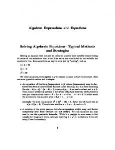
Solving Algebraic Equations– Typical Methods and Strategies. Solving an
equation that contains an unknown quantity (the variable) means finding all
values of ...
Oct 22, 2008 - (3) (a) Suppose that two irreducible modules M1,M2 of the same dimension are ..... found by solving some quadratic equation over K. Any other ...
SOLVING ALGEBRAIC EQUATIONS BY AN AUTOMATIC COMPUTER. 1. Iterate
the function 2y2 — 1, starting with the number y whose arc sin is required. 2.
Aug 19, 2014 - Mohsen Rostami-Malkhalifeh, and Gholam Reza Jahanshaloo. Department of ... Academic Editor: Mohammad Khodabakhshi. Copyright ...... [6] T. Allahviranloo, M. Ghanbari, A. A. Hosseinzadeh, E. Haghi, and R. Nuraei, âA ...
reveal the coordinates of the line perpendicular to its respective hyperplane, and so .... perpendicular lines placed from one point of the dihedron side on the.
Sep 30, 2013 - A numerical technique based on reproducing kernel methods for the exact solution of linear Volterra integral equations system of the second ...
Feb 1, 2008 - of C. Let spanâ¥. R (A) denote the orthogonal complement of spanR(A) in Rn and let G = (gij) be an r à n integer matrix of rank r whose rows g1 ...
Nov 30, 2018 - Annals of Mathematics 142 (3): 443â551. [2] Bourbaki, Nicolas (1994). Elements of the history of mathematics. Translated by Meldrum, John.
24 Nov 2009 ... Performance Objective(s): Given linear equations, students will solve the
equations using the appropriate .... linear equations. Self-Reflection:.
Solving simultaneous linear equations. 3.4. Introduction. Equations often arise in
which there is more than one unknown quantity. When this is the case there will ...
naive parallel versions of Gauss-Jordan method such as row block and row cyclic .... thread Tmy rank+1. 3) Perform the elimination step number k for all rows m,.
Chapter 1: Classification of differential equations. ... Solving simple boundary
value problems by integration . .... Section 4.4: Numerical methods for initial value
problems . ... Programming in MATLAB, part III . ..... PDF). If you are reading t
May 2, 2012 - geometric equations and make use of their symmetry properties to obtain ... details, as also to Ref [7] for construction of coherent states for the ...
May 2, 2012 - desired polynomials and functions and the space of monomials [2, 3]. In this method, ..... Using the above, one can write down the two particle Jack polynomial as,. Jλ({zi}) = â. â n=0 .... [5] F. M. Fernández, Phys. Lett. A 237 .
Which system of equations below will determine the number of adult tickets, a,
and the .... KEY: Linear system | elimination | word problem. MSC: Application.
[5] H. Anton, R.C. Busby, Contemporary Linear Algebra, John Wiley, 2003. [6] M. Friedman, M. Ming, A. Kandel, Fuzzy linear systems, Fuzzy Sets and. Systems ...
Any function y(t) â L2([0, 1]) can be expanded in Haar series y(t) = â. 8 i=1 aihi(t). where ai .... Exact solution of above system is y1 (t) = et, y2 (t) = sint, y3 (t) = et + cost. Suppose y. â² ... 3 H. (14). Now integrating equation (12) â
to solve general functional equation: y = f+N(y), where f is specified ... This method is better than numerical method as it is free from rounding off ..... â2t + 33e. ât. +. 56. 9 te. â3t. â16te. â2t â 30te. ât. +. 4. 3 t2e. â3t, y3,
MATLAB Tutorial VI Solving a System of Linear Algebraic Equations
Tutorial VI: Linear Algebraic Equations. Last updated 5/19/05 by G.G. Botte. 1.
Department of Chemical Engineering. ChE-101: Approaches to Chemical ...
Tutorial VI: Linear Algebraic Equations
Last updated 5/19/05 by G.G. Botte
Department of Chemical Engineering ChE-101: Approaches to Chemical Engineering Problem Solving MATLAB Tutorial VI Solving a System of Linear Algebraic Equations
(last updated 5/19/05 by GGB)
Objectives: These tutorials are designed to show the introductory elements for any of the topics discussed. In almost all cases there are other ways to accomplish the same objective, or higher level features that can be added to the commands below. Read Chapter 3 of the textbook to learn more about matrix operations Any text below appearing after the double prompt (>>) can be entered in the Command Window directly or in an m-file. ______________________________________________________________________________ The following topics are covered in this tutorial; Introduction Solving Using Matrix Algebra Commands Solved Problems (guided tour) Proposed Problems ______________________________________________________________________________ Introduction: There are a number of common situations in chemical engineering where systems of linear equations appear. Any system of 'n' linear equations in 'n' unknowns can be expressed in the general form: a11 x1 + a12 x2 + a21 x1 + a22 x2 +
an1 x1 + an2 x2 +
..... ..... : : .....
+ a1nxn + a2nxn
+ ann xn
= =
b1 b2
=
bn
where xj is the jth variable, aij is the constant coefficient on the jth variable in the ith equation, and bj is the constant term. There are at least three ways in Matlab of solving these systems; (1) using matrix algebra commands, (the preferred method) (2) using the symbolic algebra solve command, (3) using the numerical equation solver, ie. the fsolve command. Only the matrix algebra method will be demonstrated in this tutorial.
1
===================================================================== Method Using Matrix Algebra Commands The system of equations given above can be expressed in the following matrix form.
⎡ a11 a 12 ⎢a a 22 ⎢ 21 ⎢ ⎢ ⎢ ⎢⎣ a n1 a n 2
... ... a1n ⎤ ⎡ x1 ⎤ ⎡ b1 ⎤ ⎢b ⎥ ... ... a 2 n ⎥ ⎢ x 2 ⎥ ⎥⎢ ⎥ ⎢ 2⎥ ⎥⎢ :⎥ = ⎢ :⎥ : ⎥⎢ ⎥ ⎢ ⎥ : ⎥⎢ :⎥ ⎢ :⎥ ⎢⎣ b n ⎥⎦ ... ... a nn ⎥⎦ ⎢⎣ x n ⎥⎦
In short_hand notation this is listed as [ A ]{x} = {b} . Remember that the rules of matrix multiplication dictate that the '[A]' matrix be consistent with the '{x}' and '{b}' vectors. The first column of 'A' contains the coefficients for x1. The first row of 'A' and element of 'b' contain the coefficients for the first equation. To determine the variables contained in the column vector '{x}', complete the following steps. (a) Create the coefficient matrix '[A]'. Also remember to include zeroes where an equation doesn't contain a variable. (b) Calculate the determinant of the coefficient matrix to make sure that you have an independent set of equations. If the determinant is zero you have a singular matrix. The meaning of this is that your equations are not independent therefore; you will have to verify each of your equations. You will start learning how to formulate equations to understand different processes when you take ChE-200. The command used in Matlab to calculate the determinant of a matrix is det. See the example given below: ⎡3 1 1⎤ Calculate the determinant of the matrix A = ⎢⎢ 2 0 1 ⎥⎥ ⎢⎣ 2 3 4 ⎥⎦
Because the determinant is different to zero the inverse matrix of A exists.
2
Tutorial VI: Linear Algebraic Equations
(c) (d)
Last updated 5/19/05 by G.G. Botte
Create the right_hand_side column vector '{b}' containing the constant terms from the equation. This must be a column vector, not a row. Calculate the values in the '{x}' vector of unknowns by performing the following matrix −1 operation: {x} = [ A ] {b}
Where [A]-1 is the inverse matrix of the coefficient matrix A. The command used in Matlab to calculate the inverse of a matrix is inv. See the example given below:
This is the inverse matrix of A ⎡1⎤ Therefore, if the {b} vector is given by: {b} = ⎢⎢ 0 ⎥⎥ . The solution of the system of LAEs can be ⎢⎣ −1⎥⎦ calculated in Matlab as shown below:
3
This must be a column vector This is the operational symbol for the product of matrices (see Tutorial 3) Solution for the system of LAEs
The inv command will give you an error message if the matrix that you are trying to calculate the inverse to is singular. See the example given below:
Remember: This means that you don’t have a set of independent equations
4
Tutorial VI: Linear Algebraic Equations
Last updated 5/19/05 by G.G. Botte
SOLVED PROBLEMS 1. The following series of reversible reactions occurs;
A B A D B C B D C D Assume that the reactions are carried out in a batch reactor at constant temperature and pressure, and that the reactor initially contains only component A at a concentration of 1 mole/liter. Given the first order rate constants for each reaction, determine the equilibrium concentration of each component. Given an example set of rate constants, and applying a mass balance on three of the components and the constraint that the concentration of all four species must sum to one, results in the following system of linear equations. C A + C B + C C + C D = 1 _0.3C A + 0.02C B + 0.05C D = 0.1C A _ 0.82C B + 0.1C C + 0.1C 0.5C B _ 0.11C C + 0.1C D = 0
0 D
=
0
Write a program in Matlab to calculate the concentration of each of the components in the reactor. . Solution: 1. The first step is to express the system of linear algebraic equations in matrix form:
where N1 trough N5 represents the flowrates in moles/hr of ethane fed, chlorine fed, ethane remaining, dichloroethane produced, and hydrogen chloride produced respectively. Is the system of equations linear or nonlinear? Justify your answer. If linear express the system of equations in matrix form and develop a program in Matlab to obtain the solution for the flowrates.