Sep 30, 2008 - and W is the Gaussian noise with i.i.d. entries of zero mean and ...... [21] Weisstein, Eric W. âCircle-Circle Intersectionâ, from MathWorld-A ...
1
Algebraic reduction for space-time codes based on quaternion algebras
arXiv:0809.3365v2 [cs.IT] 30 Sep 2008
L. Luzzi
G. Rekaya-Ben Othman*
J.-C. Belfiore
Abstract In this paper we introduce a new right preprocessing method for the decoding of 2 × 2 algebraic STBCs, called algebraic reduction, which exploits the multiplicative structure of the code. The principle of the new reduction is to absorb part of the channel into the code, by approximating the channel matrix with an element of the maximal order of the algebra. We prove that algebraic reduction attains the receive diversity when followed by a simple ZF detection. Simulation results for the Golden Code show that using MMSE-GDFE left preprocessing, algebraic reduction with simple ZF detection has a loss of only 3 dB with respect to ML decoding. Index Terms: Algebraic reduction, right preprocessing, Golden Code EDICS category: MSP-DECD
I. I NTRODUCTION Space-time coding for multiple antenna systems is an efficient device to compensate the effects of fading in wireless channels through diversity techniques, and allows for increased data rates. A new generation of space-time code designs for MIMO channels, based on suitable subsets of division algebras, has been recently developed [17]. The algebraic constructions guarantee that these codes are full-rank, full-rate and information-lossless, and have the non-vanishing determinant property. Up to now, the decoding of algebraic space-time codes has been performed using their lattice point representation. In particular, maximum likelihood decoders such as the Sphere Decoder or the SchnorrEuchner algorithm are currently employed. However, the complexity of these decoders is prohibitive for Jean-Claude Belfiore, Ghaya Rekaya-Ben Othman and Laura Luzzi are with TELECOM ParisTech, 46 Rue Barrault, 75013 Paris, France. E-mail: {belfiore, rekaya, luzzi}@telecom − paristech.fr. Tel: +33 (0)145817705, +33 (0)145817633, +33 (0)145817636. Fax: +33 (0)145804036
September 30, 2008
DRAFT
2
practical implementation, especially for lattices of high dimension, arising from MIMO systems with a large number of transmit and receive antennas. On the other side, suboptimal decoders like ZF, DFE, MMSE have low complexity but their performance is poor; in particular they don’t preserve the diversity order of the system. The use of preprocessing before decoding improves the performance of suboptimal decoders, and reduces considerably the complexity of ML decoders [12]. Two types of preprocessing are possible: - Left preprocessing (MMSE-GDFE) to obtain a better conditioned channel matrix; - Right preprocessing (lattice reduction) in order to have a quasi-orthogonal lattice. The most widely used lattice reduction is the LLL reduction. We are interested here in the right preprocessing stage; we propose a new reduction method for 2 × 2 space-time codes based on quaternion algebras which directly exploits the multiplicative structure of the space-time code in addition to the lattice structure. Up to now, algebraic tools have been used exclusively for coding but never for decoding. Algebraic reduction consists in absorbing a part of the channel into the code. This is done by approximating the channel matrix with a unit of a maximal order of the quaternion algebra. The algebraic reduction has already been implemented by Rekaya et al. [16] for the fast fading channel, in the case of rotated constellations based on algebraic number fields. In this context, the units in the ring of integers of the field form an abelian multiplicative group whose generators are described by Dirichlet’s unit theorem [10]. The reduction algorithm then amounts to decoding in the logarithmic lattice of the unit group, which is fixed once and for all. In this case, one can show that the diversity of the channel is preserved. For quaternion skewfields, which are the object of this paper, the situation is more complicated because the unit group is not commutative. However, it is still possible to find a finite presentation of the group, that is a finite set of generators and relations. Supposing that a presentation is known, we describe an algorithm to find the best approximation of the channel matrix as a product of the generators. As an example, we consider the Golden Code, and find a set of generators for the unit group of its maximal order. Our simulation results for the Golden Code show that using MMSE-GDFE left preprocessing, the performance of algebraic reduction with ZF decoding is within 3 dB of the ML. The paper is organized as follows: in Section II we introduce the system model; in Section III we explain the general method of algebraic reduction. In Section IV we present the search algorithm to
September 30, 2008
DRAFT
3
approximate the channel matrix with a unit; in Section V we prove that our method yields diversity order equal to 2 when followed by a simple ZF decoder. We discuss its performance obtained through simulations in the case of the Golden Code, and compare algebraic reduction and LLL reduction using various decoders (ZF, ZF-DFE), with and without MMSE-GDFE preprocessing. Finally, in Section VI we describe a method to obtain the generators of the unit group for a maximal order in a quaternion algebra. The computations are carried out in detail for the case of the algebra of the Golden Code. II. S YSTEM
MODEL AND NOTATION
A. System model We consider a quasi-static 2 × 2 MIMO system employing a space-time block code. The received signal is given by X, H, Y, W ∈ M2 (C)
Y = HX + W,
(1)
The entries of H are i.i.d. complex Gaussian random variables with zero mean and variance per real dimension equal to 21 , and W is the Gaussian noise with i.i.d. entries of zero mean and variance N0 . X is the transmitted codeword. In this paper we are interested in STBCs that are subsets of a principal
ideal Oα of a maximal order O in a cyclic division algebra A of index 2 over Q(i) (a quaternion algebra). We refer to [17] for the necessary background about space-time codes from cyclic division algebras, and to [8] for a discussion of codes based on maximal orders. Example (The Golden Code). The Golden Code falls into this category (see [1] and [8]). It is based on the cyclic algebra A = (Q(i, θ)/Q(i), σ, i), where θ =
√ 5+1 2
and σ : x 7→ x ¯ is such that σ(θ) = θ¯ = 1−θ
and σ leaves the elements of Q(i) fixed. It has been shown in [8] that
x1 x2 , x1 , x2 ∈ Z[i, θ] O= i¯ x2 x ¯1
is a maximal order of A. O can be written as O = Z[i, θ] ⊕ Z[i, θ]j , where 0 1 j= i 0
(2)
(3)
Up to a scaling constant, the Golden Code is a subset of the two-sided ideal Oα = αO, with α = 1 + iθ¯ [11]. Every codeword of G has the form
αx1
αx2
1 X=√ 5 ¯ x1 α ¯ ix2 α September 30, 2008
DRAFT
4
with x1 = s1 + s2 θ , x2 = s3 + s4 θ . The symbols s1 , s2 , s3 , s4 belong to a QAM constellation. B. Notation In the following paragraphs we will often pass from the 2 × 2 matrix notation for the transmitted and received signals to their lattice point representation as complex vectors of length 4. To avoid confusion, 4 × 4 matrices and vectors of length 4 are written in boldface (using capital letters and small letters
respectively), while 2 × 2 matrices are not in bold. Notation (Vectorization of matrices). Let φ be the function M2 (C) → C4 that vectorizes matrices: a c 7→ (a, b, c, d)t φ: (4) b d
The left multiplication function Al : M2 (C) → M2 (C) that maps B to AB induces a linear mapping Al = φ ◦ Al ◦ φ−1 : C4 → C4 . That is,
φ(AB) = Al φ(B) ∀A, B ∈ M2 (C) Al is the block diagonal matrix
A 0 Al = 0 A
(5)
Notation (Lattice point representation). Let {w1 , w2 , w3 , w4 } be a basis of αO as a Z[i]-module. Every codeword X can be written as X=
4 X
si wi ,
i=1
s = (s1 , s2 , s3 , s4 )t ∈ Z[i]4
Let Φ be the matrix whose columns are φ(w1 ), φ(w2 ), φ(w3 ), φ(w4 )
(6)
Then the lattice point corresponding to X is x = φ(X) =
4 X
si φ(wi ) = Φs
i=1
We denote by Λ the Z[i]-lattice with generator matrix Φ. A complex matrix T is called unimodular if the elements of T belong to Z[i] and det(T) ∈ {1, −1, i, −i}.
Recall that two generator matrices Φ and Φ′ span the same Z[i]-lattice if Φ′ = ΦT with T unimodular. The following remark explains the relation between the units of the maximal order O of the code algebra
and unimodular transformations of the code lattice. This property is fundamental for algebraic reduction. September 30, 2008
DRAFT
5
Remark 1 (Units and unimodular transformations). Suppose that U ∈ O∗ is an invertible element: then {U w1 , U w2 , U w3 , U w4 } is still a basis of αO seen as a Z[i]-lattice. The codeword X can also be expressed in the new basis: X=
4 X
s′i (U wi ),
s′ = (s′1 , s′2 , s′3 , s′4 )t ∈ Z[i]4
i=1
The vectorized signal is Φs = φ(X) =
4 X
φ(U wi ) =
4 X
s′i Ul φ(wi ) = Ul
s′i φ(wi ) = Ul Φs′
i=1
i=1
i=1
4 X
Now consider the change of coordinates matrix TU = Φ−1Ul Φ ∈ M4 (C) from the basis {φ(wi )}i=1,...,4
to {φ(U wi )}i=1,...,4 . We have det(TU ) = det(Ul ) = det(U )2 = ±1, see equation (5). Moreover, we
have seen that ∀s ∈ Z[i]4 , s′ = TU s ∈ Z[i]4 . Then TU is unimodular, and the lattice generated by ΦTU is still Λ. III. A LGEBRAIC
REDUCTION
In this section we introduce the principle of algebraic reduction. First of all, we consider a normalization of the received signal. In the system model (1), the channel matrix H has nonzero determinant with probability 1, and so it can be rewritten as H=
Therefore the system is equivalent to
p
det(H)H1 ,
Y1 = p
Y det(H)
H1 ∈ SL2 (C)
= H 1 X + W1
Algebraic reduction consists in approximating the normalized channel matrix H1 with a unit U of norm 1 of the maximal order O of the algebra of the considered STBC, that is an element U of O such that det(U ) = 1.
A. Perfect approximation In order to simplify the exposition, we first consider the ideal case where we have a perfect approximation: H1 = U . Of course this is extremely unlikely in practice; the general case will be described in the next paragraph. The received signal can be written: Y1 = U X + W1
September 30, 2008
(7)
DRAFT
6
and U X is still a codeword. In fact, since U is invertible, {U X | X ∈ Oα} = Oα
Applying φ to both sides of equation (7), we find that the equivalent system in vectorized form is y1 = Ul Φs + w1
where Φ is the matrix defined in (6), s ∈ Z[i]4 , y1 = φ(Y1 ), w1 = φ(W1 ). We have seen in Remark 1 that since U is a unit, Ul Φ = ΦTU ,
with TU unimodular. So s1 ∈ Z[i]4
y1 = ΦTU s + w1 = Φs1 + w1 ,
In order to decode, we can simply consider ZF detection: # " � −1 � 1 Φ−1 w ˆ s1 = Φ y1 = s1 + p det(H)
where [ ] denotes the rounding of each vector component to the nearest (Gaussian) integer. If Φ is unitary, as in the case of the Golden Code, algebraic reduction followed by ZF detection gives optimal (ML) performance. B. General case In the general case, the approximation is not perfect with probability 1 and we must take into account the approximation error E . We write H1 = EU , and the vectorized received signal is y1 = El Ul Φs + w1 = El ΦTU s + w1 = El Φs1 + w1
The estimated signal after ZF detection is �
ˆ s1 = Φ
−1
E−1 l y1
�
"
= s1 + p
1 det(H)
Φ
−1
E−1 l w
#
= [s1 + n]
(8)
s1 . Finally, one can recover an estimate of the initial signal ˆ s = T−1 U ˆ
Thus, the system is equivalent to a non-fading system where the noise n is no longer white Gaussian.
September 30, 2008
DRAFT
7
C. Choice of U for the ZF decoder We suppose here for simplicity that the generator matrix Φ is unitary, but a similar criterion can be established in a more general case. We have seen that ideally the error term E should be unitary in order to have optimality for the ZF decoder, so we should choose the unit U in such a way that E = H1 U −1 is quasi-orthogonal. We require that the Frobenius norm kEk2F should be minimized1 :
2
U = argmin U H1−1 F
(9)
U ∈O, det(U )=1
This criterion corresponds to minimizing the trace of the covariance matrix of the new noise n in (8): ! � �H 1 1 −1 H −1 −1 Φ−1 = Cov(n) = Cov p Φ−1 E−1 l w = |det(H)| Φ El Cov(w) El det(H) �H �H N0 = Φ−1 E−1 Φ−1 E−1 l l |det(H)|
and
tr(Cov(n)) =
−1 −1 2
−1 2
N0 N0
Φ E =
E = 2N0 E −1 2 l l F F F |det(H)| |det(H)| |det(H)|
IV. T HE
(10)
APPROXIMATION ALGORITHM
In this section we describe an algorithm to find the nearest unit U to the normalized channel matrix H1 with respect to the criterion (9). To do this we need to understand the structure of the group of units
of the maximal order O. Notation. We denote elements of SL2 (C) with capital letters (for example H1 , U ) when considering their matrix representation, and with small letters (for example h1 , u) when we want to stress that they are group elements. Remark 2 (Units of norm 1). The set O1 = {u ∈ O∗ | det(u) = 1}
is a subgroup of O. In fact, if u is a unit of the Z[i]-order O, then NA/Q(i) (u) = det(u) is a unit in Z[i], that is, det(u) ∈
{1, −1, i, −i}. O1 is the kernel of the reduced norm mapping N = NA/Q(i) : O∗ → {1, −1, i, −i} which
is a group homomorphism, thus it is a subgroup of O. 1
‚ ‚2 Remark that since det(E) = 1, kEk2F = ‚E −1 ‚F .
September 30, 2008
DRAFT
8
Table I G ENERATORS OF O1 . 1 0 A = iθ, iθ¯ 1 i 1+i A = i + (1 + i)j =@ i−1 i 1 0 θ 1+i A = θ + (1 + i)j =@ i−1 θ¯ 1 0 θ −1 − i A = θ − (1 + i)j =@ −i + 1 θ¯ 1 0 1+i 1 + iθ¯ ¯ A = (1 + i) + (1 + iθ)j =@ i(1 + iθ) 1 + i 1 0 1+i 1 + iθ A = (1 + i) + (1 + iθ)j =@ ¯ i(1 + iθ) 1+i 1 0 1−i θ¯ + i A = (1 − i) + (θ¯ + i)j =@ i(θ + i) 1 − i 1 0 1−i θ+i A = (1 − i) + (θ + i)j =@ i(θ¯ + i) 1 − i
0 iθ u1 = @ 0 0 u2
u3
u4
u5
u6
u7
u8
u−1 1
0 iθ¯ =@ 0 0
0 iθ i
1
A = iθ¯ −1 − i
1
A = i − (1 + i)j @ u−1 2 = −i + 1 i 1 0 θ¯ −1 − i −1 A = θ¯ − (1 + i)j u3 = @ −i + 1 θ 1 0 θ¯ 1+i −1 A = θ¯ + (1 + i)j u4 = @ i−1 θ 1 0 1+i −1 − iθ¯ −1 ¯ A = (1 + i) + (1 + iθ)j u5 = @ −i(1 + iθ) 1+i 1 0 1+i −1 − iθ −1 A = (1 + i) − (1 + iθ)j u6 = @ ¯ −i(1 + iθ) 1+i 1 0 1−i −θ¯ − i −1 A = (1 − i) − (θ¯ + i)j u7 = @ −i(θ + i) 1−i 1 0 1−i −θ − i −1 A = (1 − i) − (θ + i)j u8 = @ −i(θ¯ + i) 1−i
Example (The Golden Code). In the case of the Golden Code, N is surjective since N(1) = 1, N(θ) = θ θ¯ = −1, N(j) = −j 2 = −i, N(jθ) = i. So {1, −1, i, −i} ∼ = O∗ /O1 , and O1 is a normal subgroup of
index 4 of O∗ . In order to obtain a set of generators, it is then sufficient to study the structure of O1 . Its cosets can be obtained by multiplying for one of the coset leaders {1, θ, j, θj}.
Our problem is then reduced to studying the subgroup O1 . In particular, we need to find a presentation of this group: a set of generators S and a set of relations R among these generators. In fact, one can show that O1 is finitely presentable, that is it admits a presentation with S and R finite [9]. Example (Generators and relations in the case of the Golden Code). The group O1 is generated by 8 units, that are displayed in Table I. The corresponding relations are shown in Table II.
The method for finding a presentation is based on the Swan algorithm [18]. As it is not well known and is rather complex, we have chosen to expose it in detail in Section VI.
September 30, 2008
DRAFT
9
Table II F UNDAMENTAL RELATIONS AMONG THE GENERATORS OF O1 .
u33 = −1
u34 = −1
(u2 u1 )3 = 1
3 (u2 u−1 1 ) = 1
u6 u3 u7 = −1
u6 u7 u−1 4 = −1 u8 u3 u5 = −1
u−1 4 u8 u5 = −1
−1 u1 u−1 3 u1 u4 = 1 −1 −1 u−1 5 u2 u5 u1 u8 u2 u8 u1 = 1
−1 −1 −1 −1 u6 u−1 2 u6 u1 u7 u2 u7 u1 = 1
A. Action of the group on the hyperbolic space H3 The search algorithm is based on the action of the group on a suitable space. We use the fact that O1 is a subgroup of the special linear group SL2 (C), and consider the action of SL2 (C) on the hyperbolic 3-space H3 (see for example [5] or [13] for a reference).
We refer to the upper half-space model of H3 : H3 = {(z, r) | z ∈ C, r ∈ R, r > 0}
(11)
H3 can also be seen as a subset of the Hamilton quaternions H: a point P can be written as (z, r) =
z + rj = x + iy + rj, where {1, i, j, k} is the standard basis of H. We endow H3 with the hyperbolic
distance ρ such that if P = z + rj, P ′ = z ′ + r ′ j,
cosh ρ(P, P ′ ) = 1 +
d(P, P ′ )2 , 2rr ′
where d(P, P ′ )2 = |z − z ′ |2 + (r − r ′ )2 is the squared Euclidean distance. The corresponding surface
and volume forms on H3 are ([13], pp. 48–49)
dx2 + dy 2 + dr 2 , r2 dxdydr dv = r3
ds =
September 30, 2008
(12) (13)
DRAFT
10
The geodesics with respect to this metric are the (Euclidean) half-circles perpendicular to the plane {r = 0} and with center on this plane, and the half-lines perpendicular to {r = 0}. Given a matrix a b ∈ SL2 (C), g= c d
its action on a point P = (z, r) is defined as follows: z∗ = ∗ ∗ g(z, r) = (z , r ), with r∗ =
¯ (az+b)(¯ cz¯+d)+a¯ cr 2 , |cz+d|2 +|c|2 r 2 r |cz+d|2 +|c|2 r 2
(14)
(Here we denote by z¯ the complex conjugate of z ).
The action of g and −g is the same, so there is an induced action of P SL2 (C) = SL2 (C)/{1, −1}.
P SL2 (C) can be identified with the group Isom+ (H3 ) of orientation-preserving isometries of H3 with
respect to the metric defined previously ([13], p. 48). All the information we will gain about the group O1 will thus be modulo the equivalence relation g ∼ −g;
we denote by P O1 its quotient with respect to this relation. Consider the action of P SL2 (C) on the special point J = (0, 1) = j
(15)
which has the following nice property ([5], Proposition 1.7): ∀g ∈ SL2 (C),
kgk2F = 2 cosh ρ(J, g(J))
(16)
Remark 3. If g ∈ U (2) is unitary, then g leaves every point of H3 fixed ([5], Proposition 1.1). Then by
considering for example the mapping P SL2 (C) → H3 that sends g to g(J), one can identify H3 with the quotient space P SL2 (C)/U (2). B. The algorithm We assume here the following fundamental properties, which will be proven in Section VI: 1) {u(J) | u ∈ O1 } is a discrete set in H3 . 2) Given a unit u ∈ O1 , the set
Pu = {P ∈ H3 | ρ(P, u(J)) ≤ ρ(P, u′ (J))
∀u′ 6= u}
is a compact hyperbolic polyhedron with finite volume and finitely many faces.
September 30, 2008
DRAFT
11
3) Two distinct polyhedra Pu , Pu′ can intersect at most in one face; all the polyhedra are isometric,
and they cover the whole space H3 , forming a tiling. Moreover, if P = P1 is the polyhedron containing J , Pu = u(P)
4) The polyhedra adjacent to P are given by −1 u1 (P), . . . , ur (P), u−1 1 (P), . . . , ur (P)
(17)
where {u1 , . . . , ur } is a minimal set of generators for O1 . As anticipated in Section III, given the normalized channel matrix h1 ∈ SL2 (C) we want to find
2
u ˆ = argmin uh−1 1 F
(18)
u∈O 1
But we know from equation (16) that
−1 2
uh = 2 cosh(ρ(J, uh−1 (J))) = 2 cosh(ρ(u−1 (J), h−1 (J))), 1 1 1 F
since u is an isometry. So the condition (18) is equivalent to
u ˆ = argmin ρ(u−1 (J), h−1 1 (J)) u∈O 1
The point h−1 ¯(P) = Pu¯ of the polyhedron P for some u ¯ ∈ O1 . It follows 1 (J) is contained in the image u
¯(J) than to any other u(J), u ∈ O1 . Since all the from the definition of Pu¯ that h−1 1 (J) is closer to u
polyhedra are isometric, ρ(¯ u(J), h−1 1 (J)) ≤ Rmax
where Rmax is the radius of the smallest (hyperbolic) sphere containing P . Therefore we have the following property:
−1 2
uh ≤ CO 1 F
(19)
We now go back to the problem of finding a unit u ¯ such that h−1 ¯(P), given a normalized 1 (J) ∈ u
channel matrix h1 ∈ SL2 (C). Let u1 , . . . , ur be the generators of O1 in (17) and ur+1 = u−1 1 , . . . , u2r = u−1 r their inverses. The neighboring polyhedra of P are all of the form ui (P), i = 1, . . . , 2r.
The idea is to begin the search from P and the neighboring polyhedra, corresponding to the generators
of the group and their inverses, and choose the Ui such that ui (J) is the closest to h−1 1 (J). Since ui is
and start again the search of the ui′ that gives the an isometry of H3 , at the next step we can apply u−1 i
September 30, 2008
DRAFT
12
h−1(J)
v −1h−1(J)
v(J) v(P) v −1
J
J P
P
v −1(J) v −1(P)
Figure 1.
A step of the algorithm. The polyhedra are represented as two-dimensional polygons for simplicity.
closest point to ui −1 h−1 1 (J). With this strategy we only need to update a single point and perform 2r comparisons at each step of the search. The algorithm is illustrated in Figure 1. Suppose that the matrix form of the ui has been stored in memory at the beginning of the program, together with the images u1 (J), . . . , u2r (J) of J , for example using the coordinates in the upper halfspace model (11). Let ui (J) = (xi , yi , ri ),
i = 1, . . . , 2r
INPUT: h1 ∈ SL2 (C). Initialization: let h = h1 ,u ¯ = 1,i0 = 0. REPEAT 1) Compute h−1 (J) = (x, y, r). 2) Compute the distances di = 2 cosh ρ(h−1 (J), ui (J)) = 1 +
(x − xi )2 + (y − yi )2 + (r − ri )2 , 2rri
i = 1, . . . , 2r,
d0 = 2 cosh ρ(h−1 (J), J)
3) Let i0 = argmini∈{0,1,...,2r} di . (If several indices i attain the minimum, choose the smallest.) 4) Update u ¯←u ¯ui0 , h ← hui0 . UNTIL i0 = 0. OUTPUT: u ˆ=u ¯−1 is the chosen unit. September 30, 2008
DRAFT
13
Remark 4 (Advantage of the algebraic reduction in the case of slow fading channels). If the channel varies slowly from one time block to the next, it is reasonable to expect that the polyhedron u ¯(P) containing h−1 1 (J) at the time t will be the same, or will be adjacent, to the polyhedron chosen at
the time t − 1. Thus, this method requires only a slight adjustment of the previous search at each step. On the contrary, the LLL reduction method requires a full lattice reduction at each time block. V. P ERFORMANCE
OF THE ALGEBRAIC REDUCTION
A. Diversity It has recently been proved [19] that MIMO decoding based on LLL reduction followed by zero-forcing achieves the receive diversity. The following Proposition shows that algebraic reduction is equivalent to LLL reduction in terms of diversity for the case of 2 transmit and 2 receive antennas: Proposition 1. The diversity order of the algebraic reduction method with ZF detection is 2. Proof: We suppose that the symbols si , i = 1, . . . , 4 belong to an M -QAM constellation, with M = 22m . Let Eav be the average energy per symbol, and γ =
Eav N0
the SNR.
For a fixed realization of the channel matrix H , equation (8) is equivalent to an additive channel without fading where the noise n is no longer white. We can compute the error probability using ZF detection conditioned to a certain value of H , and then average over the distribution of H : Pe (γ) =
Z
Pe (γ | H)dH
(20)
With symbol by symbol ZF detection, Pe (γ) is bounded by the error probability for each symbol: Pe (γ) ≤
4 X i=1
P ((ˆ s1 )i 6= (s1 )i ),
Using the classical expression of Pe in a Gaussian channel, for square QAM constellations ([15], §5.2.9), we obtain P ((ˆ s1 )i 6= (s1 )i ) ≤ 4 erfc
s
3Eav 2 σ (M − 1)
!
av − 2(M3E−1)σ 2
≤ 4e
i
where σi2 is the variance for complex dimension of the noise component ni . We have seen in (10) that the trace of the covariance matrix of the new noise n is bounded by
−1 2 −1 2 N0
Φ E , recalling that the Frobenius norm is submultiplicative. Thus |det(H)|
F
l
F
σi2 ≤ Cov(n) ≤
September 30, 2008
CN0 |det(H)|
DRAFT
14
2
2 because E −1 F = U H1−1 F ≤ CO , see equation (19).
2
= E−1 2 ≤ CO . Indeed if Φ is unitary, as in the case of the Golden Code, Φ−1 E−1 l l F F
Finally,
−
Pe (γ | H) ≤ 16e
“
3 2(M −1)C
” |det(H)| ENav 0
= 16e−c|det(H)|γ
In order to compute the error probability in equation (20), we need the distribution of |det(H)|. It is
known [7, 4] that if H is gaussian with i.i.d. N (0, 1) entries (variance per real dimension 12 ), the random variable 4 |det(H)|2 , corresponding to the determinant of the Wishart matrix 2HH H , is distributed as the product of two independent chi square random variables with 2 and 4 degrees of freedom respectively. Consider two random variables X ∼ χ2 (2),Y ∼ χ2 (4): their joint probability distribution function is y x 1 pX,Y (x, y) = ye− 2 − 2 8
x, y > 0
√ Then the cumulative distribution function of Z = 2 |det(H)| = XY is ZZ √ FZ (z) = P { XY ≤ z} = √ pX,Y (x, y)dxdy xy≤z
√
From the invertible change of variables u = y , v = xy with Jacobian v2 2v − u2 u = − 2v J = u 1 0 we obtain
FZ (z) =
Z
0
pZ (z) =
z
Z
∞
pX,Y
0
∂FZ (z) z = ∂z 4
�
Z
� � Z z �Z ∞ u v2 v v2 , u |J| dudv = e− 2u − 2 du dv, u 0 4 0
∞
0
z2
u
e− 2u − 2 du =
z2 K1 (z), 2
where K1 is the modified Bessel function of the second kind. Finally, Z i h ′ Pe (γ) ≤ E 16e−c γZ = 16 = 16
∞
z2 ′ K1 (z)e−c γz dz = 2 0 � � � �!! ∞ X 1 2 1 Γ(k + 52 ) 5 , + Ψ k+ − Ψ(k + 1) − 2 ln(c′ γ) (c′ γ)2 π(c′ γ)4 (c′ γ)2k Γ(k + 1) 2 k=0
where Ψ is the Digamma function. The series in the last expression being uniformly bounded for large γ , the leading term is of the order of
September 30, 2008
1 γ2 .
DRAFT
15
B. Some remarks about complexity The length of the algorithm described in Section IV-B is related to the initial distance
2
2
−1 2
h = kh1 k2 = √ H = kHkF 2 cosh ρ(h−1 (J), J) = 1 1 F
det H F |det(H)| F
In order to have more information about the distribution of this distance, one has to find the distribution of the random variable
kHk2F |det(H)| .
From [4], we learn that H is unitarily similar to X 0 1 e = , H 2 Y Z
where X 2 ∼ χ2 (4), Y 2 , Z 2 ∼ χ2 (2) and X, Y, Z are independent. Therefore
2
e 2
H kHkF X2 + Y 2 + Z2 F = = |det(H)| XZ e det(H)
We want to find the distribution of the random variable T = X, Y, Z : pX (x) =
x3 − x2 e 2, 2
y2
pY (y) = ye− 2 ,
X 2 +Y 2 +Z 2 XZ
knowing the distributions of
pZ (z) = ze−
z2 2
Their joint probability distribution is pX,Y,Z (x, y, z) =
1 1 3 2 2 2 x yze− 2 (x +y +z ) , 2
and the distribution of T is given by ∂ ∂ pT (t) = FT (t) = ∂t ∂t ∂ = ∂t
Z
0
∞Z
x(t+
x(t−
√
√ 2
t2 −4) 2
t2 −4)
ZZ Z
0
x2 +y2 +z 2 xz
√
pX,Y,Z (x, y, z)dxdydz = ≤t
txz−x2 −z 2
x3 yz − x2 +y2 +z2 2 e dydzdx 2
With the change of variables 2t = cosh(u), w = y 2 this integral becomes ! Z ∞ Z x(cosh(u)+sinh(u)) Z 2 cosh(u)xz−x2 −z 2 3 ∂ x z − x2 +z2 +w ∂u 2 e = dwdzdx ∂u 4 ∂t 0 x(cosh(u)−sinh(u)) 0 √ ∂ ∂u 12 t2 − 4 3 = tanh (u) = ∂u ∂t t4 The following example shows that the distance ρ(h−1 1 (J), J) is mostly concentrated near the origin: Example. In Section VI, we will see that the minimum of the distances between J and the vertices of P for the Golden Code is Rmin = arccosh(1.9069 · · · ) = 1, 2614 · · · . From the distribution of T , we find −1 that the probability that ρ(J, h−1 1 (J)) > Rmin is approximately 0.038: in most cases h1 (J) is already September 30, 2008
DRAFT
16
0
10
−1
10
−2
10
−3
FER
10
−4
10
−5
10
−6
10
ML MMSE−GDFE + AR + ZF−DFE MMSE−GDFE+AR+ZF AR+ZF ZF
−7
10
9
12
15
18
21
24
SNR
Figure 2.
Performance of algebraic reduction followed by ZF or ZF-DFE decoders using 4-QAM constellations.
contained in P or in one of the neighboring polyhedra, and the algorithm stops after one step! Moreover,
−10 , which is negligible since for practical the probability that ρ(J, h−1 1 (J)) > 5Rmin is of the order of 10
values of the SNR the probabilities of error for ML detection are typically of the order of 10−6 at best. C. Simulation results Figure 2 shows the performance of algebraic reduction followed by ZF and ZF-DFE decoding compared with ML decoding using 4-QAM constellations. One can verify that the slope of the probability of error in the case of algebraic reduction with ZF detection (without preprocessing) is very close to −2, confirming the result of Proposition 1 concerning the diversity order. One can add MMSE-GDFE left preprocessing to solve the shaping problem for finite constellations [12] in order to improve this performance. With MMSE-GDFE preprocessing, algebraic reduction is within 4.2 dB and 3.2 dB from the ML using ZF and ZF-DFE decoding, at the FER of 10−4 .
In the 16-QAM case, the loss is of 3.4 dB and 2.6 dB respectively for ZF and ZF-DFE decoding at the FER of 10−3 (Figure 3). In the same figure we compare algebraic reduction to LLL reduction using MMSE-GDFE preprocessing. The two performances are very close; with ZF-DFE decoding, algebraic reduction has a slight loss (0.3 dB). On the contrary, with ZF decoding, algebraic reduction is slightly better (0.4 dB gain), showing that the criterion (9) is indeed appropriate for this decoder. Numerical simulations also evidence that the average complexity of algebraic reduction is low. In Section IV-B we have seen that each step of the unit search algorithm requires only a few operations. Table III shows the actual distribution of the number of steps in the unit search algorithm. The data September 30, 2008
DRAFT
17
0
10
−1
FER
10
−2
10
ML MMSE−GDFE + LLL + ZF MMSE−GDFE + LLL + ZF−DFE MMSE−GDFE + AR + ZF MMSE−GDFE + AR + ZF−DFE
−3
10
−4
10
3
6
9
12
15
18
21
24
SNR
Figure 3.
Comparison of algebraic reduction and LLL reduction using MMSE-GDFE preprocessing combined with ZF or
ZF-DFE decoding with 16-QAM constellations.
Table III N UMBER OF STEPS OF average number of steps
1.923062
THE SEARCH ALGORITHM . distribution of the number of steps
1
2
3
4
5
6
7
8
9
10
> 11
38.2%
39.4%
16.0%
4.8%
1.2%
0.2%
3.7 · 10−2 %
7.6 · 10−3 %
2.6 · 10−3 %
10−4 %
0
refers to a computer simulation for the Golden Code using a ZF decoder, for 16-QAM constellations, for the transmission of 106 codewords. (Clearly this distribution does not depend on the SNR.) The average length of the algorithm is less than 2. VI. F INDING
THE GENERATORS
In this Section, we describe a method to find a presentation for the group O1 of units of norm 1, and the corresponding polyhedron P . The computations are carried out in detail for the Golden Code. A. Kleinian groups and Dirichlet polyhedra We introduce some terminology that will be useful later: Definition 1 (Kleinian groups). Let Γ be a subgroup of the projective special linear group P SL2 (C) acting on the hyperbolic space H3 . - If Γ is discrete, that is if the subspace topology on Γ is the discrete topology, Γ is called a Kleinian group. Remark that then Γ is countable. September 30, 2008
DRAFT
18
- The orbit of a point x0 ∈ H3 is the set {g(x0 ) | g ∈ Γ}.
- A fundamental set for the action of Γ is a subset of H3 containing exactly one point for every orbit. - A fundamental domain for Γ is a closed subset D of H3 such that S a) g∈Γ g(D) = H3 ,
b) If g ∈ Γ \ {1}, the interior of D is disjoint from the interior of g(D). c) The boundary of D has measure 0.
- Γ is called cocompact if it admits a compact fundamental domain; we say that Γ has finite covolume if it admits a fundamental domain with finite volume. - If Γ has finite covolume, and D1 and D2 are fundamental domains for Γ, then Vol(D1 ) = Vol(D2 ) < ∞ ([13], Lemma 1.2.9).
In the case of a Kleinian group Γ, one can obtain a fundamental domain that is a hyperbolic polyhedron [13, 2]. This polyhedron can be obtained as an intersection of hyperbolic half-spaces. For any pair of distinct points Q, Q′ ∈ H3 , the set of points equidistant to Q and Q′ with respect to ρ
is a hyperbolic plane, called the bisector between Q and Q′ , which divides H3 into two open convex
half-spaces, one containing Q and the other containing Q′ . Given g ∈ Γ, let Dg (Q) = {P ∈ H3 | ρ(Q, P ) ≤ ρ(g(Q), P )}
(21)
the closed half-space of the points that are closer to Q than to g(Q). If Q is not fixed by any nontrivial element of Γ, the Dirichlet fundamental polyhedron of Γ with center Q is defined as the intersection of all the bisectors corresponding to nontrivial elements: PΓ =
\
Dg (Q)
(22)
g∈Γ, g6=1
The definition (22) cannot be used directly to compute the polyhedron, since we ought to intersect an infinite number of bisectors. Let B(Q, R) denote the closed ball with center Q and radius R, and let DR (Q) =
\ {Dg (Q) | g 6= 1, g(Q) ∈ B(Q, R)}
(23)
If PΓ is compact, it has finite diameter, so there exists R > 0 such that PΓ = DR (Q). B. Poincar´e’s theorem From the Dirichlet polyhedron of a Kleinian group one can obtain a complete description of the latter, including generators and relations. In fact, a famous theorem due to Poincar´e establishes a correspondence
September 30, 2008
DRAFT
19
between a set of generators of the group and the isometries which map a face of the polyhedron into another face, called side-pairings. The sequences of side-pairings which send an edge into itself correspond to a complete set of relations among the generators. A complete exposition of Poincar´e’s theorem in the general case can be found in [6]. We only need a rather weak version of the theorem that we state as follows: Theorem 2 (Poincar´e’s polyhedron theorem). Let P be a hyperbolic polyhedron in H3 with finitely many faces. Let F denote the set of faces of P , and suppose that: a) [Metric condition] For every pair of disjoint faces of P , the corresponding geodesic planes have no common point at infinity. b) [Side-pairings] There exist two maps R : F → F , U : F → Isom(H3 ) such that: - ∀F ∈ F , R2 (F ) = F
- If R(F ) = F ′ , U(F ) = uF maps F ′ onto F , sending distinct vertices into distinct vertices, and distinct faces into distinct faces, and maps the interior of P outside of P . Moreover uF ′ = (uF )−1
R is called a side-pairing for P .
c) [Cycles] For each edge E1 of P , there is a cycle starting with E1 , that is a sequence of the form [E1 , . . . , En+1 ], where Ei , i = 1, . . . , n + 1 are edges of P , and ∀i ∈ {1, . . . , n} there exists a
generator u(i) ∈ U(F) such that u(i) (Ei ) = Ei+1 , and En+1 = E1 . Moreover, we suppose that u = u(n) ◦ · · · ◦ u(1) is a rotation through an angle
2π m,
m ∈ Z+ , and that its restriction to E1 is
the identity. Consider the group Γ generated by U(F). Then P is a fundamental domain for the action of Γ on H3 . The proof of this theorem is a special case of the proof of Theorem 4.14 in [6]. C. The structure of O1 We now have all the necessary background to find a fundamental domain, and thus a set of generators, for P O1 = O1 /{1, −1}. The following theorem shows that P O1 is a Kleinian group, and describes its Dirichlet polyhedron (see [5] or [20]): Theorem 3. Let A be a quaternion algebra over a number field K such that a) K has exactly one pair of complex embeddings b) A is ramified at all the real places, that is A ⊗Q Kν is a division ring for every real place ν of K . September 30, 2008
DRAFT
20
Let O be an order of A. Then: - P O1 is a Kleinian group.
- P O1 has finite covolume and its Dirichlet polyhedron has finitely many faces.
- P O1 is cocompact if and only if A is a division ring.
Remark that conditions (a) and (b) of the theorem are verified since K = Q(i) is an imaginary quadratic number field and thus has a pair of complex embeddings and no real embeddings. Thus P O1 admits a compact fundamental polyhedron PO1 of the form (22), with finitely many faces and finite volume. This volume is known a priori and only depends on the choice of the algebra A (see [13], p.336): Theorem 4 (Tamagawa Volume Formula). Let A be a quaternion algebra over K such that A ⊗Q R ∼ = M2 (C). Let O be a maximal order of A. Then the hyperbolic volume Vol(PO1 ) =
3 Y 1 2 (Np − 1) ζ (2) |D | K K 4π 2
p|δO
In the previous formula, ζK denotes the Dedekind zeta function2 relative to the field K , DK is the discriminant of K , δO is the discriminant of O, p varies among the primes of OK , and Np = [OK : pOK ], where OK is the ring of integers of K . Example (The Golden Code). In the case of the Golden Code algebra, DQ(i) = −4, and δ(O) = 5Z[i]. The only primes that divide the discriminant of the maximal order are (2 + i) and (2 − i), both with algebraic norm 5. In conclusion, Vol(PO1 ) =
8ζQ(i) (2)16 32ζQ(i) (2) = = 4, 885149838 · · · 2 4π π2
(24)
since ζQ(i) (2) = 1.50670301 · · · . Remark 5. We have seen in section IV-B that a smaller polyhedron P results in a better average distance
between u ˆ(J) and h−1 (J) and a better approximation. So the algebraic codes such that Vol(P) is small are better suited for the method of algebraic reduction. 2
The Dedekind zeta function is defined as ζK (s) =
P ([OK : I])−s , where I varies among the proper ideals of OK . I
September 30, 2008
DRAFT
21
D. Computing the Dirichlet polyhedron for O1 We suppose here that we already have an estimate of the volume of PO1 , given by Theorem 4. For this reason our strategy to find the Dirichlet polyhedron differs slightly from that described in [2]. The idea is to compute the sequence DR (Q) defined by (23) for an increasing sequence of values of R, until we find R such that DR (Q) is compact. If the hypotheses of Poincar´e’s Theorem are verified for a set of side-pairings belonging to O1 , DR (Q) is a Dirichlet polyhedron for some subgroup of O1 . To check
whether this subgroup coincides with O1 it is sufficient to estimate of the volume of DR (Q).
Following [2], we take as our base point Q the point J defined in (15). One needs to check that J is not fixed by any nontrivial element of P O1 . Remark 6. As pointed out in [2], if on the contrary J is fixed by some nontrivial element, one needs first to compute a fundamental domain for the stabilizer ΓJ of J (the subgroup of elements that fix J ), T and then intersect it with g∈Γ\ΓJ Dg (J).
Because of the property (16), in order to find DR (J) we only need to intersect the bisectors corre-
sponding to elements of O1 with square Frobenius norm less or equal to 2 cosh(R). Since O can be
identified with a discrete lattice in C4 using the map φ defined in (4), and the Frobenius norm corresponds
to the Euclidean norm in C4 , clearly there is only a finite number of these elements. Since cosh is increasing on the positive half-line, in order to find the Dg (J) one can solve half-space a b , the inequality cosh(ρ(Q, J)) ≤ cosh(ρ(Q, g(J))). For a general g = c d � ¯ � bd + a¯ c 1 g(J) = , 2 2, 2 |d| + |c| |d| + |c|2
and the corresponding half-space has equation
A2 + B 2 + 1 − 1 ≥ 0, C � � ¯ c),B = ℑ(bd+a¯ ¯ c), C = |d|2 +|c|2 . Its boundary is a sphere of center A , B , 0 where A = ℜ(bd+a¯ C−1 C−1 � 2 2 � 1 A +B and square radius C (C−1)2 + 1 . Remark that if we change the sign of the pair a, d or b, c, the radius (C − 1)x2 + (C − 1)y 2 + (C − 1)r 2 − 2Ax − 2By +
doesn’t change, while the center is reflected with respect to the origin.
If a ball or complementary of a ball (according to the sign of C − 1) in the list (23) is already contained in the intersection, we can discard the corresponding element of the group. Since all the spheres have center on the plane {r = 0}, in order to determine whether a sphere is contained in another we only need to consider their intersections with this plane. September 30, 2008
DRAFT
22
Figure 4.
The projection of the bisectors on the plane
{r = 0}.
Figure 5. The intersection of the spheres (the picture shows only half of the space for better understanding).
E. Computing the generators for the Golden Code We now apply the method described in the previous Section to the maximal order O of the algebra of
the Golden Code. One can easily verify that in this case J is not fixed by any nontrivial element of O1 .
Considering the elements g ∈ O1 such that kgk2F ≤ 9 by computer search, we find that P = DR (J) is � compact with R = arccosh 92 , since it doesn’t intersect the plane “at infinity” {r = 0}. Table I lists
the elements {ui , u−1 i }, i = 1, . . . , 8 of the group that are necessary to obtain P . The equations of the corresponding spheres, the bisectors S(ui ) = Dui (J),
(J), S(u−1 i ) = Du−1 i
i = 1, . . . , 8
(see definition (21)) can be found in Table IV. The vertices of P are the intersections of all the triples of spheres S(ui ): Vi , Vi′ = π ′ (Vi ), Vi′′ = π ′′ (Vi ), Vi′′′ = π ′′′ (Vi ),
i = 1 . . . 6,
Here π ′ ,π ′′ and π ′′′ denote the reflections with respect to the plane {y = x}, the plane {y = −x} and the line {x = 0, y = 0} respectively. ! √ √ q √ 5 5+9 3 5−1 1 V1 = , , 33 + 11 5 = S(u1 ) ∩ S(u4 ) ∩ S(u6 ), 16 16 8 � � 1+θ 1 θ ,− , = S(u1 ) ∩ S(u2 ) ∩ S(u6 ), V2 = 2 2 2 September 30, 2008
DRAFT
23
Table IV B ISECTORS unit
center
radius
int/ext
u1
(0, 0, 0) (0, 0, 0)
θ θ¯
I
u−1 1
E
(1, 1, 0)
1
E
u−1 2
(−1, −1, 0)
1
E
u3
(−θ, −θ, 0) ¯ θ, ¯ 0) (θ,
θ
E
−θ¯
E
θ
E
u2
u−1 3 u4 u−1 4
(θ, θ, 0) ¯ −θ, ¯ 0) (−θ,
” √ √ −9 5+19 −9−5 5 , 22 , 0 22 ” “ √ √ 9 5−19 9+5 5 , 22 , 0 22 ” “ √ √ 9 5+19 −9+5 5 , 22 , 0 22 ” “ √ √ −9 5−19 9−5 5 , 22 , 0 22 “ ” √ √ −9−5 5 −9 5+19 , , 0 22 “ 22 √ ” √ 9+5 5 9 5−19 , ,0 22 22 “ ” √ √ −9+5 5 9 5+19 , 22 , 0 22 “ ” √ √ 9−5 5 −9 5−19 , ,0 22 22 “
u5 u−1 5 u6 u−1 6 u7 u−1 7 u8 u−1 8
−θ¯
√ 7 (7 22 √ 7 (7 22 √ 7 (7 22 √ 7 (7 22 √ 7 (7 22 √ 7 (7 22 √ 7 (7 22 √ 7 (7 22
E
√
5)
E
√
5)
E
+
√
5)
E
+
√
5)
E
√
5)
E
√
5)
E
+
√
5)
E
+
√
5)
E
− −
− −
0.8 0.6 0.4 –1
–1 –0.5
–0.5 0
0 0.5
0.5 1
Figure 6.
1
A schematic representation of the polyhedron
P (in the picture, the edges have been replaced by straight
Figure 7. The projection of the polyhedron P on the plane {r = 0}.
lines).
September 30, 2008
DRAFT
24
V3 V4 V5 V6
�
� θ θ¯ 1 ,− , = = S(u4 ) ∩ S(u6 ) ∩ S(u−1 7 ), 2 2 2 r ! √ √ 3 5 1 3 5 1 1 11 = = S(u2 ) ∩ S(u6 ) ∩ S(u−1 + , − , 7 ) 20 2 20 2 2 10 ! √ √ q √ 1+3 5 5 5−9 1 −1 −1 33 − 11 5 = S(u−1 , , = 1 ) ∩ S(u4 ) ∩ S(u7 ), 16 16 8 � � 1 θ¯2 θ¯ −1 = ,− , = S(u−1 1 ) ∩ S(u2 ) ∩ S(u7 ) 2 2 2
The faces of P correspond to portions F (u) of the spheres S(u), with u one of the units in Table I. The projection of the faces of P on the plane {r = 0} is shown in Figure VI-E.
As explained in Section VI-D, in order to prove that P is a Dirichlet polyhedron for O1 , we will first
show that it is a fundamental domain for some subgroup Γ of O1 using Poincar´e’s Theorem. Comparing
the volume of P with the value (24), we will find that Γ = O1 .
The metric condition in Poincar´e’s Theorem can be verified given the equations of the spheres (see also Figure 4). Define a side-pairing as follows: U(F (u)) = u, R(F (u)) = F (u−1 ) for every u in Table I. The action of the generators on the faces and vertices is summarized in Table VI, and it is not hard to see that it satisfies all the conditions in the theorem. In fact every face F (u) = P ∩ u(P) ⊂ S(u). Remark that an isometry between polygons with the same number of vertices, sending distinct vertices in distinct vertices, must be onto. In order to check that the cycle condition of Theorem 2 holds, we need to compute the minimal relations or “cycles” between the generators, by finding the sequences of edges of P of the form [E1 , . . . , En+1 ],
such that u(i) (Ei ) = Ei+1 , and En+1 = E1 . As F ((u(i) )−1 ) must contain Ei , there are only two possible choices for u(i) , corresponding to the two faces containing the edge Ei . Given such a sequence, u(1) · · · u(n) is an element of finite order in O1 , that is (u(1) · · · u(n) )k = 1 for some k. (Remark that every cyclic permutation of the sequence [E1 , . . . , En+1 ] gives rise to a new cycle.) Actually it is necessary to “lift” the relation from P SL2 (C) to SL2 (C). We also require our sequences to be irreducible, that is u(i+1) 6= (u(i) )−1 for all i. In this way we obtain a decomposition of the set of edges of P into cycles. The action of the generators on the faces is summarized in Table VI; the cycles are described in Table V. A complete set of relations is listed in Table II. Except for the first four, the products correspond to the identity in P SL2 (C) (thus, a trivial rotation). By computing the eigenvalues of u3 , u4 , u2 u1 and u2 u−1 1 , September 30, 2008
DRAFT
25
Table V C YCLES FOR THE EDGES OF P .
u
3 V3′′ V3′′′ −→ V3′′ V3′′′
u
4 V3 V3′ −→ V3 V3′
u
u
1 2 V6 V6′′ −→ V2′′′ V2′ −→ V6 V6′′
u−1
u
2 V2 V2′′ − −1− → V6′′′ V6′ −→ V2 V2′′
u−1
u−1
u−1
−6− → V3′′′ V1 − −3−→ V3′′′ V5′′′ − V3 V4 − −7− → V3 V4 u−1
u−1
u
4 −6− → V4′′′ V3′′′ − V1 V3 − −7−→ V5 V3 −→ V1 V3
u
u
u
u
u−1
u−1
u−1
u
u−1
u
u
5 3 8 V3′ V4′ −→ V3′′ V5′′ −→ V3′′ V1′′ −→ V3′ V4′
4 V5′ V3′ −→ V1′ V3′ − −8−→ V4′′ V3′′ − −5−→ V5′ V3′
u
1 1 V1 V1′ − −4− → V5 V5′ −→ V1′′′ V1′′ − −3−→ V5′′′ V5′′ −→ V1 V1′
u
u−1
u
1 8 2 8 V5′ V6′ −→ V1′′ V2′′ −→ V4′ V2′ −→ V4′′ V2′′ −→ V1′ V2′ − −1−→ · · ·
u−1
u−1
u
2 · · · V5′′ V6′′ − −5−→ V4′ V6′ −→ V4′′ V6′′ − −5−→ V5′ V6′
u−1
u−1
u−1
u−1
u−1
u
−1− → V5′′′ V6′′′ − −2−→ V4′′′ V6′′′ − V1 V2 − −7−→ V4 V6 − −7−→ · · · u
u
1 6 6 · · · V1′′′ V2′′′ −→ −2− → V4′′′ V2′′′ −→ V5 V6 −→ V4 V2 − V1 V2
Table VI ACTION OF
u1 (S(u−1 1 )) = S(u1 )
THE GENERATORS ON THE VERTICES OF
P.
u1 (V5 ) = V1′′′ , u1 (V5′ ) = V1′′ , u1 (V5′′ ) = V1′ , u1 (V5′′′ ) = V1 , u1 (V6 ) = V2′′′ , u1 (V6′ ) = V2′′ , u1 (V6′′ ) = V2′ , u1 (V6′′′ ) = V1
u2 (S(u−1 2 )) = S(u2 )
u2 (V6′ ) = V2′′ ), u2 (V4′ ) = V4′′ ), u2 (V2′ ) = V6′′ , u2 (V6′′′ ) = V2 , u2 (V4′′′ ) = V4 , u2 (V2′′′ ) = V6
September 30, 2008
u3 (S(u−1 3 )) = S(u3 )
u3 (V3′′ ) = V3′′ , u3 (V3′′′ ) = V3′′′ , u3 (V5′′ ) = V1′′ , u3 (V5′′′ ) = V1′′′
u4 (S(u−1 4 )) = S(u4 )
u4 (V3 ) = V3 , u4 (V3′ ) = V3′ , u4 (V5′ ) = V1′ , u4 (V5 ) = V1
u5 (S(u−1 5 )) = S(u5 )
u5 (V3′ ) = V3′′ , u5 (V6′ ) = V6′′ , u5 (V5′ ) = V4′′ , u5 (V4′ ) = V5′′
u6 (S(u−1 6 )) = S(u6 )
u6 (V3′′′ ) = V3 , u6 (V4′′′ ) = V1 , u6 (V1′′′ ) = V4 , u6 (V2′′′ ) = V2
u7 (S(u−1 7 )) = S(u7 )
u7 (V3 ) = V3′′′ , u7 (V5 ) = V4′′′ , u7 (V6 ) = V6′′′ , u7 (V4 ) = V5′′′
u8 (S(u−1 8 ))
u8 (V4′′ ) = V1′ , u8 (V2′′ ) = V2′ , u8 (V3′′ ) = V3′ , u8 (V1′′ ) = V4′′
= S(u8 )
DRAFT
26
we find that they are indeed conjugated to rotations of an angle
2π 3
around the axis {x = 0, y = 0}.3
We have thus shown that P is a Dirichlet polyhedron for some subgroup Γ of O1 . But if Γ were a proper subgroup, the volume of P would be a multiple of the volume of the fundamental polyhedron for O1 that we computed in (24), that is it should be at least 2 · 4.88514 · · · = 9.77029 · · · .
So the last step of the proof that P is a fundamental polyhedron for O1 is the following: Lemma 5. Vol(P) < 9.77029 · · · . The proof of this fact is rather tedious and is reported in the Appendix. Remark 7. From the coordinates of the vertices of P , one finds that the radius of the smallest hyperbolic sphere containing P is Rmax = arccosh(2.2360 · · · ) = 1.4436 · · · ,
while the minimum of the distances between J and the vertices of P is Rmin = arccosh(1.9069 · · · ) = 1.2614 · · ·
VII. C ONCLUSIONS In this paper we have introduced a right preprocessing method for the decoding of space-time block codes based on quaternion algebras, which allows to improve the performance of suboptimal decoders and reduces the complexity of ML decoders. The new method exploits the algebraic structure of the code, by approximating the channel matrix with a unit in the maximal order of the quaternion algebra. Our simulations show that algebraic reduction and LLL reduction have similar performance. However in the case of slow fading, unlike LLL reduction, algebraic reduction requires only a slight adjustment of the previous approximation at each time block, without needing to perform a full reduction. In future work we will deal with the generalization of algebraic reduction to higher-dimensional space time codes based on cyclic division algebras. 3
g ∈ SL2 (C) is called elliptic, and is a rotation around a fixed geodesic, if and only if tr(g) ∈ R and |tr(g)| < 2, see [5],
Prop. 1.4. If its eigenvalues are eiβ , e−iβ , then the angle of rotation is 2β.
September 30, 2008
DRAFT
27
A PPENDIX A. Proof of Lemma 5 In order to prove that the volume of P is smaller than the required constant, we can compute the ¯
volume of the hyperbolic polyhedron Q enclosed by S(u1 ), the plane {r = − θ2 }, and the spheres −1 −1 −1 S(u2 ),S(u−1 2 ),S(u1 ),S(u4 ),S(u3 ),S(u4 ),S(u3 ). Clearly Q ⊃ P . Recalling the definition of the o n ¯ hyperbolic volume in (13), the volume of the spherical sector T enclosed by S(u1 ) and r = − 2θ
is
Z
θ ¯
− θ2
� ¯�� � θ 1 π(θ 2 − r 2 ) 4 dr = π − − ln(θ) + 2θ + ln − = 36.2937 · · · r3 2 2
To this volume we must subtract the volume of the intersection of T with the chosen spheres. From the expression for the area of the intersection of two circles of radii R1 and R2 whose centers have distance d [21] �
� � 2 � d2 + R12 − R22 d + R22 − R12 2 A(R1 , R2 , d) = + R2 arccos + 2dR1 2dR2 p 1p (−d + R1 − R2 ) (d + R1 − R2 )(d − R1 + R2 )(d + R1 + R2 ), + 2 √ √ we obtain the area of the horizontal sections of T ∩ S(u2 ). Since R1 = θ 2 − r¯2 , R2 = 1 − r¯2 R12 arccos
are the radii of S(u1 ) ∩ {r = r¯}, S(u2 ) ∩ {r = r¯} respectively, and the distance between the centers is √ d = 2, we find ! √ 2 θ−2 2 2 √ + A(R1 , R2 , d) = π(1 − r¯ ) + (¯ r − 1) arccos 4 1 − r¯2 ! √ 2 1 + θ2 1p 2 2 √ + (θ − r¯ ) arccos −1 + 6θ 2 − θ 4 − 8v 2 , − 4 θ 2 − r¯2 2 √ √ 5 . In conclusion, which is defined for r¯ ≤ 9+3 4 Vol(T ∩ S(u2 )) = Vol(T ∩ S(u−1 2 )) =
Z
√
¯ − θ2
√ 9+3 5 4
A(R1 , R2 , d) dr = 5.96793 · · · r3
Proceeding in the same way, one can compute Vol(T ∩ S(u4 )) = Vol(T ∩ S(u3 )) = 5.34536 · · · , � −1 −1 Vol (T ∩ S(u−1 1 )) \ (S(u1 ) ∩ (S(u2 ) ∪ S(u2 )) = 2.49982 · · · , � −1 −1 Vol (T ∩ S(u−1 3 )) \ (S(u3 ) ∩ (S(u3 ) ∪ S(u1 )) = 0.70490 · · ·
September 30, 2008
DRAFT
28
Therefore the volume of Q is less than 36.29366 − 2 · 5.96793 − 2 · 5.34536 − 2.49982 − 2 · 0.70490 = 9.75746 < 9.77029,
which completes our proof. R EFERENCES [1] J-C. Belfiore, G. Rekaya, E. Viterbo, “The Golden Code: a 2 × 2 full-rate Space-Time Code with non-vanishing determinants”, IEEE Trans. Inform. Theory, vol 51 n.4, 2005 [2] C. Corrales, E. Jespers, G. Leal, A. del Rio, “Presentations of the unit group of an order in a non-split quaternion algebra”, Advances in Mathematics, 186 n. 2 (2004) 498–524 [3] M. O. Damen, H. El Gamal, G. Caire, “MMSE-GDFE lattice decoding for solving under-determined linear systems with integer unknowns”, Proceedings of ISIT 2004, Chicago, USA [4] A. Edelman, “Eigenvalues and condition numbers of random matrices”, Ph.D. Thesis, MIT 1989 [5] J. Elstrodt, F. Grunewald, J. Mennicke, “Groups acting on Hyperbolic Space”, Springer Monographs in Mathematics, 1998 [6] D. Epstein, C. Petronio, “An exposition of Poincar´e’s Polyhedron Theorem”, L’Enseignement Math´ematique, 40 (1994), 113–170 [7] N. R. Goodman, “The distribution of the determinant of a complex Wishart distributed matrix”, Ann. Math. Statist., 34, 178-180 [8] C. Hollanti, J. Lahtonen, K. Ranto, R. Vehkalahti, On the densest MIMO lattices from cyclic division algebras, submitted to IEEE Trans. Inform. Theory [9] E. Kleinert, “Units of classical orders: a survey”, L’Enseignement Math´ematique, 40 (1994), 205– 248 [10] S. Lang, “Algebraic number theory”, Springer-Verlag 2000 [11] L. Luzzi, G. Rekaya Ben-Othman, J.-C. Belfiore, E. Viterbo, Golden Space-Time Block Coded Modulation, submitted to IEEE Trans. Inform. Theory [12] A. D. Murugan, H. El Gamal, M. O. Damen, G. Caire, “A unified framework for tree search decoding: rediscovering the sequential decoder”, IEEE Trans. Inform. Theory, vol 52 n. 3, 2006 [13] C. Maclachlan, A. W. Reid, “The arithmetic of hyperbolic 3-manifolds”, Graduate texts in Mathematics, Springer, 2003
September 30, 2008
DRAFT
29
[14] F. Oggier, G. Rekaya, J.-C. Belfiore, E. Viterbo, “Perfect Space-Time Block Codes”, IEEE Trans. Inform. Theory, vol. 52 n.9, 2006 [15] J. Proakis, “Digital communications”, McGraw-Hill 2001 [16] G. Rekaya, J-C. Belfiore, E. Viterbo, “A very efficient lattice reduction tool on fast fading channels”, Proceedings of ISITA 2004, Parma, Italy [17] B. A. Sethuraman, B. Sundar Rajan, V. Shashidar, “Full-diversity, high-rate space-time block codes from division algebras”, IEEE Trans. Inform. Theory, vol 49 n. 10, 2003, pp. 2596–2616 [18] R. G. Swan, “Generators and relations for certain special linear groups”, Adv. Math. 6, 1–77 [19] M. Taherzadeh, A. Mobasher, A. K. Khandani, “LLL reduction achieves the receive diversity in MIMO decoding”, IEEE Trans. Inform. Theory, vol 53 n. 12, 2007, pp 4801–4805 [20] M-F. Vign´eras, “Arithm´etique des Alg`ebres de Quaternions”, Lecture Notes in Mathematics, Springer Verlag 1980 [21] Weisstein, Eric W. “Circle-Circle Intersection”, from MathWorld-A Wolfram Web Resource. http://mathworld.wolfram.com/Circle-CircleIntersection.html
September 30, 2008
DRAFT