RMSE (root mean squared prediction error), MAE ... MAE, and OR should be low. ... [6] Li Tan, Zhengguo Li, Yih Han Tan, Rahardja, S.âRelevant MSE-Based.
(IJACSA) International Journal of Advanced Computer Science and Applications, Vol. 5, No. 4, 2014
Image Sharpness Metric Based on Algebraic MultiGrid Method Qian Ying , Ren Xue-mei, Huang Ying, Meng Li Laboratory of Graphics Image and Multimedia, Chongqing University of Posts and Telecommunications Chongqing, China
Abstract—In order to improve Mean Square Error of its reliance on reference images when evaluating image sharpness, the no-reference metric based on algebraic multi-grid is proposed. The proposed metric first reconstructs the original image by Algebraic Multi-grid (AMG), then compute the Mean Square Error between original image and reconstructed image, the result represents image sharpness. Experiments show that the proposed sharpness metric has better practicability and monotonicity, correlates well with the perceived sharpness. The algorithm has superiority in image sharpness metric. Keywords—image sharpness mean square error; algebraic multigrid method; sharpness metric; image reconstruction
I. INTRODUCTION There has been an increasing need to develop quality measurement techniques that can predict perceived image/video quality automatically. These methods are useful in various image/video processing applications [1-5], such as compression, communication, printing, display, analysis, registration, restoration and enhance [6]. Subjective quality metrics are considered to give the most reliable results since, for many applications, it is the end user who is judging the quality of the output. Subjective quality metrics are costly, time-consuming and impractical for real-time implementation and system integration. On the other hand, objective metrics can be divided into three categories: full-reference, reducedreference, and no-reference, which is the most convenient. The traditional sharpness metrics are gradient function, such as Sum Modulus Difference (SMD), Variance are gray scale function, and entropy function. In recent years, Marziliano[7] and Ong et al. measure the image based on smoothing effects of edge blur. Ferzli[8] put forward perceptual sharpness metric based on measured just-noticeable blurs (JNBs), but unable to keep balance between stability and sensitivity. Narvekar and Karam[9] estimate the sharpness of an image as the cumulative probability of detecting blur at an edge (CPBD). Mean square error (MSE) is a full-reference evaluation methods commonly used, which requires a reference to calculate sharpness of distortion image. In this paper, we propose an improved MSE together with reconstruction image use algebraic multi-grid. The proposed metric scans for the whole image. The clearer the image is, the smaller the similarity between pixels and the smaller of MSE between image reconstructed by algebraic multi-grid and Original Image. So the metric proposed could used to measure image sharpness.
II.
PROPOSED NO-REFERENCE OBJECTIVE SHARPNESS METRIC
A. Algebraic multi-grid is an iterative method used for solving the matrix equation automatic and established on geometric multi-grid [10]. Algebraic multi-grid is mainly used for solving large-scale scientific project computation, especially partial differential equations (group). AMG is allowed to solve the non-structure mesh, and therefore it is more easily extended to image processing [11-12]. AMG is mainly applied in image reconstruction, binary, recovery and denoising [13-14]. When applied Algebraic multi-grid in image reconstruction, first, we should convert the image into graph, then, create relationship affinity (affinity) matrix on similarity between pixels gray value of image. The similarity between pixels can be calculated by weight function, the commonly function used is: Wij exp(
|| Fi Fj ||22
2 l
Fi
|| xi x j ||22 ) if || xi x j ||2 r exp( )* x2 0 otherwise
(1)
Fj
Where, and are pixels' gray values of point i and j in x image, i is pixel’s value of coordinates in space, l is
standard deviations of Gaussian function, x is standard deviations of space coordinates function, r is striking distance between two nodes. From the weight function we know that the closer two points’ distance and gray values are to each other, the greater the similarity of two points. Secondly, extract coarsening sequence of image and define the original coefficient matrix as finest mesh, the original definition of the coefficient matrix of the finest mesh 0 . In order to derive a coarse level system, we first need a splitting of
m
into two disjoint subsets
m F m +C m
, with
C m representing those variables which are to be contained in m the coarse level (C-variables) and F being the complementary set (F-variables). According to the above description, we regard the set of coarse-level variables as a subset of fine-level ones. The coarse grid is a subset of its finer grid. m m Generally, C and F are selected as follows
175 | P a g e www.ijacsa.thesai.org
(IJACSA) International Journal of Advanced Computer Science and Applications, Vol. 5, No. 4, 2014
1)
), we know that C
i F m and j Sim (strongly connected to i
For any
j Cm
or j is strongly connected to point in
m
. m 2) C is the largest point set formed by strong connection point. Where the strong connection point is defined as follows: aij 0 maxk i(aik ),0 0 1
(2) This definition is actually for M-matrix, which is symmetric positive definite matrix and non-diagonal elements are no positive.
0
is usually taken 0.25.
The M-matrix is: a 0 i (1) i ,i ; a
0 i j
(2) i , j ; 1 A 0 (3) Finally, we could get reconstructed images through interpolating image coarsening sequence. The interpolating algorithms most commonly used are nearest neighbor interpolation, bilinear interpolation and bicubic interpolation. The nearest-neighbor interpolation algorithm selects the value of the nearest point and does not consider the values of neighboring points at all, yielding a piecewise-constant interpolation. Bilinear interpolation an extension of linear interpolation for interpolating functions of two variables on a regular 2D grid. Bicubic interpolation is an extension of cubic interpolation for interpolating data points on a two dimensional regular grid. The algorithm not only considers the influence of 4 directly adjacent pixel gray value the surrounding pixel gray scale value of four, but the variance rate of gray level. B. No-reference image sharpness metric based on AMG MSE is a traditional full-reference objective image quality evaluation. The method is easy to calculate, but it just a pure mathematical statistic of pixels error without consideration for correlation between pixels. The no-reference image sharpness metric based on AMG is an improvement to MSE. The improved algorithm is no-reference, without non-distorted image and more real-time. Firstly, we process the target image to achieve the first layer coarsening sequence by AMG. Then the reconstructed image could get by interpolation method. The MSE of the original image the reconstructed image is used to measure the sharpness of image.
III.
RESULTS AND ANALYSIS
A practical evaluation must meet the following criteria: 1) Prediction Monotonicity: Image sharpness metric scores should show a corresponding increase and decrease monotonically as the image sharpness increases and decreases. 2) Prediction Consistency: A metric must perform well regardless of the Content of image it is given. A good indicator should always perform well with different image content. 3) Prediction Accuracy: This refers to the ability to correctly evaluate image quality, can generally be determined by the index of the MOS value for comparison. A. Prediction Monotonicity Test set: There are 6 512 × 512 house images, include one original picture and five blurred images using a lowpass7 × 7Gaussian mask with standard deviation equal to 0.4, 0.8, 1.2, 1.6 and 2.0, respectively, as shown in Fig. 2。From the results shown in Figure 2, we know that the more blur image becomes, the smaller the sharpness metric value. The algorithm meets monotonicity principles.
Fig. 1. 6 different ambiguity houses
MSE is defined as follows:
M
1 MN
M 1 N 1
( f i 0 j 0
' ij
fij )2 Fig. 2. Different sharpness value of 6 houses
(3)
f Where, i and j are pixel coordinates, ij is the original f f' image, ij is the distortion image of ij .
B. Prediction Consistency First, we cut the lena image into 4 same area of four dimensions and adopt gauss filter to process the 4 images. For the 4 sub-pictures, we do as follows:
176 | P a g e www.ijacsa.thesai.org
(IJACSA) International Journal of Advanced Computer Science and Applications, Vol. 5, No. 4, 2014
The 4 sub-pictures are blurred using a lowpass7 × 7Gaussian mask with standard deviation equal to 1, 2.5, 4, and 5.5, respectively, as shown in Fig. 3。The result is shown in Table below. From it we know that the algorithm performs well regardless of the Content of image it is given. The result is consistent with its blurring. TABLE I. image name (a)
STANDARD DEVIATION 1、2.5、4、5.5 std_dev
Proposed Metric
1
34.99856
(b)
2.5
9.674969
(c)
4
5.505095
(d)
5.5
2.263391
Secondly, we metric the 4 images sharpness by the proposed algorithm, Tab.2 shows the result. And Tab.3 shows the metric result of images, which we give a Gaussian filtering conflict to result of Tab.2 with a lowpass7 × 7Gaussian mask of standard deviation equal to 5.5, 2.5, 4 and 1. TABLE II.
STANDARD DEVIATION 5.5、2.5、4、1
image name
std_dev
Proposed Metric
(a)
5.5
1.61791
(b)
2.5
9.67496
(c)
4
5.50509
(d)
1
36.3086
C. Prediction Accuracy To test the performance of the metric, all of Gaussianblurred images from the LIVE[15]. Each image was rated by about 20–29 subjects. The subjects were asked to rate the images on a continuous linear scale which was divided into five different regions namely, “Bad,” “Poor,” “Fair,” “Good,” and “Excellent.” The raw
scores for each subject were converted to difference scores and then z-scores. The scores were then scaled and shifted to a range of 1 to 100. Then the difference mean opinion score (DMOS) and mean opinion score (MOS) for each image was calculated. We use 6 kinds of algorithms to process on the 84 images from LIVE. To measure how well the proposed metric, the authors followed the suggestions of the VQEG report where several evaluation metrics are proposed. The predicted MOS values are then used in calculating the performance measures including PCC (Pearson correlation coefficient, indicates the prediction accuracy), SROCC (Spearman rank-order correlation coefficient, indicates the prediction monotonicity), RMSE (root mean squared prediction error), MAE (mean absolute prediction error) and OR (outlier ratio, indicates consistency) and Spearman correlation coefficients should be high and the values of RMSE, MAE, and OR should be low. The result is given below. TABLE III.
PERFORMANCE COMPARISON OF 6 ALGORITHMS
Metrics
Pearson
Spearman
RMSE
MAE
OR
CPBD
0.908
0.930
0.095
7.518
5.766
JNBM
0.829
0.808
0.191
10.052
7.691
SMD
0.721
0.792
0.298
12.456
9.391
entropy
0.218
0.214
0.512
17.539
14.867
Variance
0.106
0.239
0.5
17.869
15.204
Proposed Metric
0.918
0.949
0.107
7.129
5.705
It can be seen from tab.3, in the above 5 indicators, the proposed metric algorithm is better than JNBM and SMD. But for the CPBD, the proposed metric is bad in the RMSE index, mainly because of the large variation range of metric values in proposed metric. Monotonicity and accuracy of proposed Metric is higher than that of CPBD.
177 | P a g e www.ijacsa.thesai.org
(IJACSA) International Journal of Advanced Computer Science and Applications, Vol. 5, No. 4, 2014
CPBC
JNBM
SMD
Entropy
Variance
Proposed Metric
Fig. 3. Comparation of 6 algorithms and the MOS values
Fig.3 gives the fitting curve of 6 algorithms and the MOS values. From fig.2, we know that the proposed metric is good fitting to the MOS values. Where, the red line with symbol ‘*’indicates MOS values. IV. CONCLUSION After the text edit has been completed, the paper is ready for the template. Duplicate the template file by using the Save As command, and use the naming convention prescribed by your conference for the name of your paper. In this newly created file, highlight all of the contents and import your prepared text file. You are now ready to style your paper.
[1]
[2]
[3]
[4]
[5]
REFERENCES Wee C Y, ‘’Paramesran R. ‘’Image sharpness measure using eigenvalues[C]’’, 9th International Conference on Signal Processing, 2008: 840-843. Zhu and P. Milanfar, “A no-reference sharpness metric sensitive to blur and noise,” in 1st International Workshop on Quality of Multimedia Experience (QoMEX), 2009. Crete F, Dolmiere T, Ladret P, et al. ‘’The blur effect: perception and estimation with a new no-reference perceptual blur metric[C]’’. International Society for Optics and Photonics, 2007: 64920I-64920I-11. Shaked D, Tastl I. ‘’Sharpness measure: Towards automatic image enhancement[C]’’, IEEE International Conference on Image Processing. IEEE, 2005, 1: I-937-40. Hassen R, Wang Z, Salama M. ‘’No-reference image sharpness assessment based on local phase coherence measurement’’ C, 2010
178 | P a g e www.ijacsa.thesai.org
(IJACSA) International Journal of Advanced Computer Science and Applications, Vol. 5, No. 4, 2014 IEEE International Conference on Acoustics Speech and Signal Processing (ICASSP), 2010: 2434-2437. [6] Li Tan, Zhengguo Li, Yih Han Tan, Rahardja, S.”Relevant MSE-Based Image Quality Metric,”J. IEEE Transactions on Image Processing. vol.22 , no. 11, pp. 447-4459, 2012 [7] Feichtenhofer, C. ; Fassold, H. ; Schallauer, P. “A Perceptual Image Sharpness Metric Based on Local Edge Gradient Analysis,” J.Signal Processing Letters, IEEE, VOL.20,NO.4,PP.379 - 382,2013. [8] R. Ferzli, L. J. Karam. “A no-reference objective image sharpenss metric based on the notion of just noticeable blur (jnb),” J, IEEE Transactions on Image Processing, vol.18, pp.717–728, 2009 [9] N. D. Narvekar, L. J. Karam. “ ,” J, IEEE Transactions on Image Processing, vol.20, no.9, pp. 2678–2683, 2011 [10] R. D. Falgout. “An Introduction to Algebraic Multigrid,” J, Computing
in Science & Engineering,”vol.8, no.6, pp.24-33, 2006. [11] Kimmel R, Yavneh I. “An algebraic multigrid approach for image analysis, ” J,SIAM, vol. 24, no.4, pp. 1218-1231, 2003. [12] Vaněk P, Mandel J, Brezina M. ‘’Algebraic multigrid by smoothed aggregation for second and fourth order elliptic problems’’J. Computing, 1996, 56(3): 179-196. [13] Chan T F, Saad Y. ‘’Multigrid algorithms on the hypercube multiprocessor’’J. Computers, IEEE Transactions on, 1986, 100(11): 969[14] Xu Qiubin. “Numericals for total variation-based reconstruction of motion blurred images,” J, Applied Mathematics-a Journal of Chinese University, vol.25, no.3, pp. 367-373,2010. [15] Yiping Xu, Hanlin Chen, Kelong Zheng. “A Combination Algorithm for Image Denoising and Deblurring,” J, Wireless Communications Networking and Mobile Computing(WiCOM), 2010, pp.1-4.
179 | P a g e www.ijacsa.thesai.org