Algorithm selection of off-policy reinforcement learning algorithms

Algorithm selection of off-policy reinforcement learning algorithms

Romain Laroche Mostly done at: Orange Labs, 44 Avenue de la République, Châtillon, France Now at: Maluuba, 2000 Peel Street, Montréal, Canada

ROMAIN . LAROCHE @ MALUUBA . COM

arXiv:1701.08810v1 [stat.ML] 30 Jan 2017

Raphaël Féraud Orange Labs, 2 Avenue Pierre Marzin, Lannion, France

Abstract Dialogue systems rely on a careful reinforcement learning design: the learning algorithm and its state space representation. In lack of more rigorous knowledge, the designer resorts to its practical experience to choose the best option. In order to automate and to improve the performance of the aforementioned process, this article formalises the problem of online off-policy reinforcement learning algorithm selection. A meta-algorithm is given for input a portfolio constituted of several off-policy reinforcement learning algorithms. It then determines at the beginning of each new trajectory, which algorithm in the portfolio is in control of the behaviour during the full next trajectory, in order to maximise the return. The article presents a novel meta-algorithm, called Epochal Stochastic Bandit Algorithm Selection (ESBAS). Its principle is to freeze the policy updates at each epoch, and to leave a rebooted stochastic bandit in charge of the algorithm selection. Under some assumptions, a thorough theoretical analysis demonstrates its near-optimality considering the structural sampling budget limitations. Then, ESBAS is put to the test in a set of experiments with various portfolios, on a negotiation dialogue game. The results show the practical benefits of the algorithm selection for dialogue systems, in most cases even outperforming the best algorithm in the portfolio, even when the aforementioned assumptions are transgressed.

Shorter version under review by the International Conference on Machine Learning (ICML).

RAPHAEL . FERAUD @ ORANGE . COM

1. Introduction Reinforcement Learning (RL) (Sutton & Barto, 1998) is a machine learning framework intending to optimise the behaviour of an agent interacting with an unknown environment. For the most practical problems, trajectory collection is costly and sample efficiency is the main key performance indicator. This is for instance the case for dialogue systems (Singh et al., 1999) and robotics (Brys et al., 2015). As a consequence, when applying RL to a new problem, one must carefully choose in advance a model, an optimisation technique, and their parameters in order to learn an adequate behaviour given the limited sample set at hand. In particular, for 20 years, research has developed and applied RL algorithms for Spoken Dialogue Systems, involving a large range of dialogue models and algorithms to optimise them. Just to cite a few algorithms: Monte Carlo (Levin & Pieraccini, 1997), Q-Learning (Walker et al., 1998), SARSA (Frampton & Lemon, 2006), MVDP algorithms (Laroche et al., 2009), Kalman Temporal Difference (Pietquin et al., 2011), Fitted-Q Iteration (Genevay & Laroche, 2016), Gaussian Process RL (Gaši´c et al., 2010), and more recently Deep RL (Fatemi et al., 2016). Additionally, most of them require the setting of hyper parameters and a state space representation. When applying these research results to a new problem, these choices may dramatically affect the speed of convergence and therefore, the dialogue system performance. Facing the complexity of choice, RL and dialogue expertise is not sufficient. Confronted to the cost of data, the popular trial and error approach shows its limits. Algorithm selection (Rice, 1976; Smith-Miles, 2009; Kotthoff, 2012) is a framework for comparing several algorithms on a given problem instance. The algorithms are tested on several problem instances, and hopefully, the algorithm selection learns from those experiences which algorithm should be the most efficient given a new problem instance. In our setting, only one problem instance is considered, but several experiments are led to determine the fittest


algorithm to deal with it. Thus, we developed an online learning version (Gagliolo & Schmidhuber, 2006; 2010) of algorithm selection. It consists in testing several algorithms on the task and in selecting the best one at a given time. Indeed, it is important to notice that, as new data is collected, the algorithms improve their performance and that an algorithm might be the worst at a short-term horizon, but the best at a longer-term horizon. In order to avoid confusion, throughout the whole article, the algorithm selector is called a meta-algorithm, and the set of algorithms available to the meta-algorithm is called a portfolio. Defined as an online learning problem, our algorithm selection task has for objective to minimise the expected regret. At each online algorithm selection, only the selected algorithm is experienced. Since the algorithms learn from their experience, it implies a requirement for a fair budget allocation between the algorithms, so that they can be equitably evaluated and compared. Budget fairness is in direct contradiction with the expected regret minimisation objective. In order to circumvent this, the reinforcement algorithms in the portfolio are assumed to be off-policy, meaning that they can learn from experiences generated from an arbitrary non-stationary behavioural policy. Section 2 provides a unifying view of reinforcement learning algorithms, that allows information sharing between all algorithms of the portfolio, whatever their decision processes, their state representations, and their optimisation techniques. Then, Section 3 formalises the problem of online selection of off-policy reinforcement learning algorithms. It introduces three definitions of pseudo-regret and states three assumptions related to experience sharing and budget fairness among algorithms. Beyond the sample efficiency issues, the online algorithm selection approach addresses furthermore four distinct practical problems for spoken dialogue systems and online RL-based systems more generally. First, it enables a systematic benchmark of models and algorithms for a better understanding of their strengths and weaknesses. Second, it improves robustness against implementation bugs: if an algorithm fails to terminate, or converges to an aberrant policy, it will be dismissed and others will be selected instead. Third, convergence guarantees and empirical efficiency may be united by covering the empirically efficient algorithms with slower algorithms that have convergence guarantees. Fourth and last, it enables staggered learning: shallow models converge the fastest and consequently control the policy in the early stages, while deep models discover the best solution later and control the policy in late stages. Afterwards, Section 4 presents the Epochal Stochastic Bandit Algorithm Selection (ESBAS), a novel meta-algorithm addressing the online off-policy reinforcement learning al-

gorithm selection problem. Its principle is to divide the time-scale into epochs of exponential length inside which the algorithms are not allowed to update their policies. During each epoch, the algorithms have therefore a constant policy and a stochastic multi-armed bandit can be in charge of the algorithm selection with strong pseudo-regret theoretical guaranties. A thorough theoretical analysis provides for ESBAS upper bounds of the pseudo-regrets defined in Section 3 under the assumptions stated in the same section. Next, Section 5 experiments ESBAS on a simulated dialogue task, and presents the experimental results, which demonstrate the practical benefits of ESBAS: in most cases outperforming the best algorithm in the portfolio, even though its primary goal was just to be almost as good as it. Finally, Sections 6 and 7 conclude the article with respectively related works and prospective ideas of improvement.

2. Unifying view of reinforcement learning algorithms The goal of this section is to enable information sharing between algorithms, even though they are considered as black boxes. We propose to share their trajectories expressed in a universal format: the interaction process. Reinforcement Learning (RL) consists in learning through trial and error to control an agent behaviour in a stochastic environment. More formally, at each time step t ∈ N, the agent performs an action a(t) ∈ A, and then perceives from its environment a signal o(t) ∈ Ω called observation, and receives a reward R(t) ∈ R. Figure 1 illustrates the RL framework. This interaction process is not Markovian: the agent may have an internal memory. In this article, the reward function is assumed to be bounded between Rmin and Rmax , and we define the RL problem as episodic. Let us introduce two time scales with different notations. First, let us define meta-time as the time scale for algorithm selection: at one meta-time τ corresponds a meta-algorithm decision, i.e. the choice of an algorithm and

Agent o(t + 1)

R(t + 1)

a(t) Stochastic environment

Figure 1. Reinforcement Learning framework: after performing action a(t), the agent perceives observation o(t + 1) and receives reward R(t + 1) from the environment.


the generation of a full episode controlled with the policy determined by the chosen algorithm. Its realisation is called a trajectory. Second, RL-time is defined as the time scale inside a trajectory, at one RL-time t corresponds one triplet composed of an observation, an action, and a reward. Let E denote the space of trajectories. A trajectory ετ ∈ E collected at meta-time τ is formalised as a sequence of (observation, action, reward) triplets: ετ = hoτ (t), aτ (t), Rτ (t)it∈J1,|ετ |K ∈ E,

(2.1)

where |ετ | is the length of trajectory ετ . The objective is, given a discount factor 0 ≤ γ < 1, to generate trajectories with high discounted cumulative reward, also called return, and noted µ(ετ ): µ(ετ ) =

|ετ | X

γ t−1 Rτ (t).

(2.2)

t=1

Since γ < 1 and Rmin ≤ R ≤ Rmax , the return is bounded: Rmin Rmax ≤ µ(ετ ) ≤ . (2.3) 1−γ 1−γ

The state representation may be built dynamically as the trajectories are collected. Many algorithms doing so can be found in the literature, for instance (Legenstein et al., 2010; Böhmer et al., 2015; El Asri et al., 2016; Williams α et al., 2016). Then, α may learn its policy πD from the T trajectories projected on its state space representation and saved as a transition set: a transition is defined as a quadruα plet hsτ (t), aτ (t), Rτ (t), sτ (t + 1)i, with state sτ (t) ∈ SD , action aτ (t) ∈ A, reward Rτ (t) ∈ R, and next state α sτ (t+1) ∈ SD . Off-policy reinforcement learning optimisation techniques compatible with this approach are numerous in the literature (Maei et al., 2010): Q-Learning (Watkins, 1989), Fitted-Q Iteration (Ernst et al., 2005), Kalman Temporal Difference (Geist & Pietquin, 2010), etc. Another option would be to perform end-to-end reinforcement learning (Riedmiller, 2005; Mnih et al., 2013; Silver et al., 2016). As well, any post-treatment of the state set, any alternative decision process model, such as POMDPs (Lovejoy, 1991; Azizzadenesheli et al., 2016), and any off-policy technique for control optimisation may be used. The algorithms are defined here as black boxes and the considered meta-algorithms will be indifferent to how the algorithms compute their policies, granted they satisfy the assumptions made in the following section.

The trajectory set at meta-time T is denoted by: DT = {ετ }τ ∈J1,T K ∈ E T .

(2.4)

3.1. Batch algorithm selection

A sub-trajectory of ετ until RL-time t is called the history at RL-time t and written ετ (t) with t ≤ |ετ |. The history records what happened in episode ετ until RL-time t: ετ (t) = hoτ (t0 ), aτ (t0 ), Rτ (t0 )it0 ∈J1,tK ∈ E.

(2.5)

The goal of each reinforcement learning algorithm α is to find a policy π ∗ : E → A which yields optimal expected returns. Such an algorithm α is viewed as a black box that takes as an input a trajectory set D ∈ E + , where E + is the ensemble of trajectory sets of undetermined size: E + = S T α T ∈N E , and that outputs a policy πD . Consequently, a reinforcement learning algorithm is formalised as follows: α : E + → (E → A).

3. Algorithm selection model

(2.6)

Such a high level definition of the RL algorithms allows to share trajectories between algorithms: a trajectory as a sequence of observations, actions, and rewards can be interpreted by any algorithm in its own decision process and state representation. For instance, RL algorithms classically rely on an MDP α defined on a state space representation SD thanks to a proα jection ΦD : α Φα (2.7) D : E → SD .

Algorithm selection (Rice, 1976) for combinatorial search (Kotthoff, 2012) consists in deciding which experiments should be carried out, given a problem instance and a fixed amount of computational resources: generally speaking computer-time, memory resources, time and/or money. Algorithms are considered efficient if they consume little resource. This approach, often compared and applied to a scheduling problem (Gomes & Selman, 2001), experienced a lot of success for instance in the SAT competition (Xu et al., 2008). Algorithm selection applied to machine learning, also called meta-learning, is mostly dedicated to error minimisation given a corpus of limited size. Indeed, these algorithms do not deliver in fine the same answer. In practice, algorithm selection can be applied to arbitrary performance metrics and modelled in the same framework. In the classical batch setting, the notations of the machine learning algorithm selection problem are described in (Smith-Miles, 2009) as follows: • I is the space of problem instances; • P is the portfolio, i.e. the collection of available algorithms;


• µ : I × P → R is the objective function, i.e. a performance metrics enabling to rate an algorithm on a given instance; • Ψ : I → Rk are the features characterising the properties of problem instances. The principle consists in collecting problem instances and in solving them with the algorithms in the portfolio P. The measures µ provide evaluations of the algorithms on those instances. Then, the aggregation of their features Ψ with the measures µ constitutes a training set. Finally, any supervised learning techniques can be used to learn an optimised mapping between the instances and the algorithms.

Pseudo-code 1 Online algorithm selection setting Data: P ← {αk }k∈J1,KK : algorithm portfolio Data: D0 ← ∅: trajectory set for τ ← 1 to ∞ do Select σ (Dτ −1 ) = σ(τ ) ∈ P; σ(τ ) Generate trajectory ετ with policy πDτ −1 ; Get return µ(ετ ); Dτ ← Dτ −1 ∪ {ετ }; end

The final goal is to optimise the cumulative expected return. It is the expectation of the sum of rewards obtained after a run of T trajectories:

3.2. Online algorithm selection " Nevertheless, in our case, I is not large enough to learn an efficient model, it might even be a singleton. Consequently, it is not possible to regress a general knowledge from a parametrisation Ψ. This is the reason why the online learning approach is tackled in this article: different algorithms are experienced and evaluated during the data collection. Since it boils down to a classical exploration/exploitation trade-off, multi-armed bandit (Bubeck & Cesa-Bianchi, 2012) have been used for combinatorial search algorithm selection (Gagliolo & Schmidhuber, 2006; 2010) and evolutionary algorithm meta-learning (Fialho et al., 2010). In the online setting, the algorithm selection problem for off-policy reinforcement learning is new and we define it as follows: • D ∈ E + is the trajectory set; • P = {αk }k∈J1,KK is the portfolio; • µ : E → R is the objective function defined in Equation 2.2. Pseudo-code 1 formalises the online algorithm selection setting. A meta-algorithm is defined as a function from a trajectory set to the selection of an algorithm: σ : E + → P.

(3.1)

The meta-algorithm is queried at each meta-time τ = |Dτ −1 |+1, with input Dτ −1 , and it ouputs algorithm σ(τ ) σ (Dτ −1 ) = σ(τ ) ∈ P controlling with its policy πDτ −1

Eσ

# T T X X X σ(τ ) σ(τ ) µ ετ = P(D|σ)EµD , τ =1

τ =1 D∈E τ −1

(3.3a) " Eσ

# T T h i X X σ(τ ) σ(τ ) µ ετ = Eσ EµDσ , τ −1

τ =1

" Eσ

# " T # T X X σ(τ ) ) µ εσ(τ = Eσ EµDσ . τ τ −1

τ =1

(3.3b)

τ =1

(3.3c)

τ =1

Equations 3.3a, 3.3b and 3.3c transform the cumulative expected return into two nested expectations. The outside expectation Eσ assumes the algorithm selection fixed and averages over the trajectory set stochastic collection and the corresponding algorithms policies, which may also rely on a stochastic process. The inside expectation Eµ assumes the policy fixed and averages the evaluation over its possible trajectories in the stochastic environment. Equation 3.3a transforms the expectation into its probabilistic equivalent, P(D|σ) denoting the probability density of generating trajectory set D conditionally to the meta-algorithm σ. Equation 3.3b transforms back the probability into a local expectation, and finally Equation 3.3c simply applies the commutativity between the sum and the expectation. Nota bene: there are three levels of decision: meta-algorithm σ selects an algorithm α that computes a policy π that in turn controls the actions. We focus in this paper on the meta-algorithm level.

σ(τ )

the generation of the trajectory ετ in the stochastic environment. Let Eµα D be a condensed notation for the expected α return of policy πD that was learnt from trajectory set D by algorithm α: α [µ (ε)] . Eµα (3.2) D = EπD

3.3. Meta-algorithm evaluation In order to evaluate the meta-algorithms, let us formulate two additional notations. First, the optimal expected return Eµ∗∞ is defined as the highest expected return achievable


by a policy of an algorithm in portfolio P:    ∀D ∈ E + , ∀α ∈ P, Eµα ≤ Eµ∗∞ , D   ∀ > 0, ∃D ∈ E + , ∃α ∈ P,

Eµ∗∞ − Eµα D < . (3.4)

Second, for every algorithm α in the portfolio, let us define σ α as its canonical meta-algorithm, i.e. the meta-algorithm that always selects algorithm α: ∀τ , σ α (τ ) = α. The absolute pseudo-regret ρσabs (T ) defines the regret as the loss for not having controlled the trajectory with an optimal policy. Definition 1 (Absolute pseudo-regret). The absolute pseudo-regret ρσabs (T ) compares the meta-algorithm’s expected return with the optimal expected return: " T # X σ(τ ) σ ∗ ρabs (T ) = T Eµ∞ − Eσ EµDσ . (3.5) τ −1

τ =1

The absolute pseudo-regret ρσabs (T ) is a well-founded pseudo-regret definition. However, it is worth noting that an optimal meta-algorithm will not yield a null regret because a large part of the absolute pseudo-regret is caused by the sub-optimality of the algorithm policies when the trajectory set is still of limited size. Indeed, the absolute pseudo-regret considers the regret for not selecting an optimal policy: it takes into account both the pseudo-regret of not selecting the best algorithm and the pseudo-regret of the algorithms for not finding an optimal policy. Since the meta-algorithm does not interfere with the training of policies, it cannot account for the pseudo-regret related to the latter. In order to have a pseudo-regret that is relative to the learning ability of the best algorithm and that better accounts for the efficiency of the algorithm selection task, we introduce the notion of relative pseudo-regret. Definition 2 (Relative pseudo-regret). The relative pseudoregret ρσrel (T ) compares the σ meta-algorithm’s expected return with the expected return of the best canonical metaalgorithm: " T # " T # X X σ(τ ) σ α ρrel (T ) = max Eσα EµDσα − Eσ EµDσ . α∈P

τ −1

τ −1

τ =1

τ =1

may achieve a negative relative pseudo-regret, which is ill-defined as a pseudo-regret definition. Still, the relative pseudo-regret ρσrel (T ) is useful as an empirical evaluation metric. A large relative pseudo-regret shows that the metaalgorithm failed to consistently select the best algorithm(s) in the portfolio. A small, null, or even negative relative pseudo-regret demonstrates that using a meta-algorithm is a guarantee for selecting the algorithm that is the most adapted to the problem. 3.4. Assumptions The theoretical analysis is hindered by the fact that algorithm selection, not only directly influences the return distribution, but also the trajectory set distribution and therefore the policies learnt by algorithms for next trajectories, which will indirectly affect the future expected returns. In order to allow policy comparison, based on relation on trajectory sets they are derived from, our analysis relies on three assumptions whose legitimacy is discussed in this section and further developed under the practical aspects in Section 5.7. Assumption 1 (More data is better data). The algorithms produce better policies with a larger trajectory set on average, whatever the algorithm that controlled the additional trajectory: α ∀D ∈ E + , ∀α, α0 ∈ P, Eµα D ≤ Eα0 EµD∪εα0 . (3.8)

Assumption 1 states that algorithms are off-policy learners and that additional data cannot lead to performance degradation on average. An algorithm that is not off-policy could be biased by a specific behavioural policy and would therefore transgress this assumption. Assumption 2 (Order compatibility). If an algorithm produces a better policy with one trajectory set than with another, then it remains the same, on average, after collecting an additional trajectory from any algorithm: ∀D, D0 ∈ E + , ∀α, α0 ∈ P, h i h i α α α 0 Eµ 0 Eµ Eµα < Eµ ⇒ E ≤ E . 0 0 0 α α α 0 α D D D∪ε D ∪ε (3.9)

(3.6) It is direct from Equations 3.5 and 3.6 that the relative pseudo-regret can be expressed in function of absolute pseudo-regrets of the meta-algorithm σ and the canonical meta-algorithms σ α : α

ρσrel (T ) = ρσabs (T ) − max ρσabs (T ). α∈P

(3.7)

Since one shallow algorithm might be faster in early stages and a deeper one more effective later, a good meta-algorithm

Assumption 2 states that a performance relation between two policies learnt by a given algorithm from two trajectory sets is preserved on average after adding another trajectory, whatever the behavioural policy used to generate it. From these two assumptions, Theorem 1 provides an upper bound in order of magnitude in function of the worst algorithm in the portfolio. It is verified for any algorithm selection σ:


Theorem 1 (Not worse than the worst). The absolute pseudo-regret is bounded by the worst algorithm absolute pseudo-regret in order of magnitude: σ σα ∀σ, ρabs (T ) ∈ O max ρabs (T ) . (3.10)

Assumption 3 (Learning is fair). If one trajectory set is better than another for one given algorithm, it is the same for other algorithms. ∀α, α0 ∈ P, ∀D, D0 ∈ E + , (3.11)

α∈P

0

0

α α α Eµα D < EµD 0 ⇒ EµD ≤ EµD 0 .

Proof. See the appendix. Contrarily to what the name of Theorem 1 suggests, a metaalgorithm might be worse than the worst algorithm (similarly, it can be better than the best algorithm), but not in order of magnitude. Its proof is rather complex for such an intuitive and loose result because, in order to control all the possible outcomes, one needs to translate the selections of algorithm α with meta-algorithm σ into the canonical meta-algorithm σ α ’s view, in order to be comparable with it. This translation is not obvious when the meta-algorithm σ and the algorithms it selects act tricky. See the proof for an example. The fairness of budget distribution has been formalised in (Cauwet et al., 2015). It is the property stating that every algorithm in the portfolio has as much resources as the others, in terms of computational time and data. It is an issue in most online algorithm selection problems, since the algorithm that has been the most selected has the most data, and therefore must be the most advanced one. A way to circumvent this issue is to select them equally, but, in an online setting, the goal of algorithm selection is precisely to select the best algorithm as often as possible. In short, exploration and evaluation require to be fair and exploitation implies to be unfair. Our answer is to require that all algorithms in the portfolio are learning off-policy, i.e. without bias induced by the behavioural policy used in the learning dataset. By assuming that all algorithms learn off-policy, we allow information sharing (Cauwet et al., 2015) between algorithms. They share the trajectories they generate. As a consequence, we can assume that every algorithm, the least or the most selected ones, will learn from the same trajectory set. Therefore, the control unbalance does not directly lead to unfairness in algorithms performances: all algorithms learn equally from all trajectories. However, unbalance might still remain in the exploration strategy if, for instance, an algorithm takes more benefit from the exploration it has chosen than the one chosen by another algorithm. In this article, we speculate that this chosen-exploration effect is negligible. More formally, in this article, for analysis purposes, the algorithm selection is assumed to be absolutely fair regardless the exploration unfairness we just discussed about. This is expressed by Assumption 3.

In practical problems, Assumptions 2 and 3 are defeated, but empirical results in Section 5 demonstrate that the ESBAS algorithm presented in Section 4 is robust to the assumption transgressions.

4. Epochal stochastic bandit algorithm selection An intuitive way to solve the algorithm selection problem is to consider algorithms as arms in a multi-armed bandit setting. The bandit meta-algorithm selects the algorithm controlling the next trajectory ε and the trajectory return µ(ε) constitutes the reward of the bandit. However, a stochastic bandit cannot be directly used because the algorithms performances vary and improve with time (Garivier & Moulines, 2008). Adversarial multi-arm bandits are designed for nonstationary environments (Auer et al., 2002b; Allesiardo & Féraud, 2015), but the exploitation the structure of our algorithm selection problem makes it possible to√obtain pseudoregrets of order of magnitude lower than Ω( T ). Alternatively, one might consider using policy search methods (Ng & Jordan, 2000), but they rely on a state space representation in order to apply the policy gradient. And in our case, neither policies do share any, nor the meta-algorithm does have at disposal any other than the intractable histories ετ (t) defined in Equation 2.5. 4.1. ESBAS description To solve the off-policy RL algorithm selection problem, we propose a novel meta-algorithm called Epochal Stochastic Bandit Algorithm Selection (ESBAS). Because of the nonstationarity induced by the algorithm learning, the stochastic bandit cannot directly select algorithms. Instead, the stochastic bandit can choose fixed policies. To comply to this constraint, the meta-time scale is divided into epochs inside which the algorithms policies cannot be updated: the algorithms optimise their policies only when epochs start, in such a way that the policies are constant inside each epoch. As a consequence and since the returns are bounded in Equation 2.3, at each new epoch, the problem can be cast into an independent stochastic K-armed bandit Ξ, with K = |P|. The ESBAS meta-algorithm is formally sketched in Pseudocode 2 embedding UCB1 (Auer et al., 2002a) as the stochastic K-armed bandit Ξ. The meta-algorithm takes as an input


Pseudo-code 2 ESBAS with UCB1 Data: P ← {αk }k∈J1,KK ; Data: D0 ← ∅ ; for β ← 0 to ∞ ; do for αk ∈ P ; do k πD : policy learnt by αk on D2β −1 ; β 2 −1

end n ← 0, ∀αk ∈ P, nk ← 0, and xk ← 0 ; for τ ← 2β to 2β+1 − 1; do   s αkmax = argmax xk + ξ αk ∈P

log(n) ; nk

// Portfolio: the set of algorithms. // Trajectory set: initiated to ∅. // For each epoch β, // For each algorithm α, k // Update the current policy πD

2β −1

.

// Initialise a new UCB1 k-armed bandit. // For each meta-time step τ ,

// UCB1 bandit selects the policy.

kmax Generate trajectory ετ with policy πD ; // This policy controls the next trajectory. β 2 −1

Get return µ(ετ ), Dτ ← Dτ −1 ∪ {ετ }; nkmax xkmax + µ(ετ ) xkmax ← ; nkmax + 1 kmax kmax n ←n + 1 and n ← n + 1; end end

// The return is observed as the UCB1 reward. // Update the empirical mean of selected arm. // Update the number of arm selections.

the set of algorithms in the portfolio. Meta-time scale is fragmented into epochs of exponential size. The β th epoch lasts 2β meta-time steps, so that, at meta-time τ = 2β , epoch β starts. At the beginning of each epoch, the ESBAS metaalgorithm asks each algorithm in the portfolio to update their current policy. Inside an epoch, the policy is never updated anymore. At the beginning of each epoch, a new Ξ instance is reset and run. During the whole epoch, Ξ decides at each meta-time step which algorithm is in control of the next trajectory.

algorithm might be optimal at meta-time τ but yield no new information, implying the same situation at meta-time τ + 1, and so on. Thus, a meta-algorithm that exclusively selects the deterministic algorithm would achieve a short-sighted pseudo-regret equal to 0, but selecting other algorithms are, in the long run, more efficient. Theorem 2 expresses in order of magnitude an upper bound for the short-sighted pseudo-regret of ESBAS. But first, let define the gaps:

4.2. ESBAS short-sighted pseudo-regret analysis

It is the difference of expected return between the best algorithm during epoch β and algorithm α. The smallest non null gap at epoch β is noted:

It has to be noted that ESBAS simply intends to minimise the regret for not choosing the best algorithm at a given meta-time τ . It is somehow short-sighted: it does not intend to optimise its algorithms learning. The following shortsighted pseudo-regret definition captures the function ESBAS intends to minimise. Definition 3 (Short-sighted pseudo-regret). The shortsighted pseudo-regret ρσss (T ) is the difference between the immediate best expected return algorithm and the one selected: " T # X σ(τ ) σ α ρss (T ) = Eσ max EµDτσ−1 − EµDσ . (4.1) τ =1

α∈P

τ −1

The short-sighted pseudo-regret optimality depends on the meta-algorithm itself. For instance, a poor deterministic

0

α ∆α Eµα ESBAS . ESBAS − Eµ β = max Dσ Dσ 0 α ∈P

∆†β =

2β −1

min

α∈P,∆α β >0

(4.2)

2β −1

∆α β.

(4.3)

If ∆†β does not exist, i.e. if there is no non-null gap, the problem is trivial and the regret is null. Upper bounds on short-sighted and absolute pseudo-regrets are derived. Theorem 2 (ESBAS short-sighted pseudo-regret). If the stochastic multi-armed bandit Ξ guarantees a regret of order of magnitude O(log(T )/∆†β ), then:   blog(T )c X β ESBAS . ρσss (T ) ∈ O  (4.4) † β=0 ∆β


∆†β Θ (1/T ) †

Θ(T −c ), c† ≥ 0.5 †

Θ(T −c ), c† < 0.5 Θ (1)

ESBAS

ρσss

ρσabs (T ) in function of ρσabs (T )

∆†β

∗

†

O(T 1−c )

†

Θ(T −c ),

O(T c log(T ))

∗

ρσabs (T ) ∈ O(T 1−c )

O (log(T ))

Θ (1/T )

†

∗

ρσabs (T ) ∈ O(log(T ))

O (log(T ))

O log2 (T )/∆†∞

∗

ESBAS

(T )

†

†

O(T 1−c )

c† ≥ 0.5

O(T 1−c ) ∗

O(T 1−c ), Table 1. Bounds on ρss (T ) obtained with Theorem 2 for the ESBAS meta-algorithm with a two-fold portfolio.

†

Θ(T −c ),

if c† < 1 − c∗

†

O(T c log(T ))

c† < 0.5

†

O(T c log(T )), if c† ≥ 1 − c∗

Proof. See the appendix. Θ (1) Several upper bounds in order of magnitude on ρss (T ) can directly be deduced from Theorem 2, depending on an order of magnitude of ∆†β . Table 1 reports some of them for a two-fold portfolio. It must be read by line. According to the first column: the order of magnitude of ∆†β , the ESBAS short-sighted pseudo-regret bounds are displayed in the second column. One should notice that the first two bounds are obtained by summing the gaps. This means that ESBAS is unable to recognise the better algorithm, but the pseudo-regrets may still be small. On the contrary, the two last bounds are deduced from Theorem 2. In this case, the algorithm selection is useful. The worse algorithm α† is, the easier algorithm selection gets, and the lower the upper bounds are. About ESBAS ability to select the best algorithm: if ∆†β ∈ √ O(1/ T ), then the meta-algorithm will not be able to distinguish the two best algorithms. Still, √ we have the guarantee that pseudo-regret ρss (T ) ∈ O( T ). The impossibility to determine which is the better algorithm is interpreted in (Cauwet et al., 2014) as a budget issue. The meta-time necessary to distinguish arms that are ∆†β apart with an arbitrary confidence interval takes Θ(1/∆†2 ) meta√β † time steps. As a consequence, if ∆β ∈ O(1/ T ), then 1/∆†2 β ∈ Ω(T ). However, the budget, i.e. the length of epoch β starting at meta-time T = 2β , equals T . In fact, even more straightforwardly, the stochastic bandit problem is known to be Θ(min(∆T, log(1 + ∆2 T )/∆)) (Perchet & Rigollet, 2013), which highlights the limit of distinguishability at ∆2 T ∈ Θ(1). Spare the log(T ) factor in Table 1 bounds, which comes from the fact the meta-algorithm starts over a novel bandit problem at each new epoch, ESBAS faces the same hard limit. 4.3. ESBAS absolute pseudo-regret analysis As Equation 3.7 recalls, the absolute pseudo-regret can be decomposed between the absolute pseudo-regret of the

O log2 (T )/∆†∞

∗

O(T 1−c )

Table 2. Bounds on ρabs (T ) given various configurations of settings, for a two-fold portfolio algorithm selection with ESBAS.

canonical meta-algorithm of the best algorithm and the relative pseudo-regret, which is the regret for not running the best algorithm alone. The relative pseudo regret can in turn be upper bounded by a decomposition of the selection regret: the regret for not always selecting the best algorithm, and potentially not learning as fast, and the short-sighted regret: the regret for not gaining the returns granted by the best algorithm. These two successive decomposition lead to Theorem 3 that provides an upper bound of the absolute pseudo-regret in function of the canonical meta-algorithm of the best algorithm, and the short-sighted pseudo-regret, which order magnitude is known to be bounded thanks to Theorem 2. Theorem 3 (ESBAS absolute pseudo-regret upper bound). If the stochastic multi-armed bandit Ξ guarantees that the best arm has been selected in the T first episodes at least T /K times, with high probability δT ∈ O(1/T ), then: ∃κ > 0, ∀T ≥ 9K 2 , ∗

ESBAS

ρσabs (T ) ≤ (3K + 1)ρσabs ESBAS

+ρσss

T 3K

(4.5)

(T ) + κ log(T ).

where algorithm selection σ ∗ selects exclusively algorithm α α∗ = argminα∈P ρσabs (T ). Proof. See the appendix. Table 2 reports an overview of the absolute pseudo-regret bounds in order of magnitude of a two-fold portfolio in function of the asymptotic behaviour of the gap ∆†β and the absolute pseudo-regret of the meta-algorithm of the the

Algorithm selection of off-policy reinforcement learning algorithms ∗

best algorithm ρσabs (T ), obtained with Theorems 1, 2 and 3. Table 1 is interpreted by line. According the order of magnitude of ∆†β in the first column, the second and third columns display the ESBAS absolute pseudo-regret bounds cross ∗ depending on the order of magnitude of ρσabs (T ). Several remarks on Table 2 can be made. Firstly, like in Table 1, Theorem 1 is applied when ESBAS is unable to distinguish the better algorithm, and Theorem 2 are applied when ESBAS algorithm selection is useful: the worse algorithm α† is, the easier algorithm selection ∗ gets, and the lower the upper bounds. Secondly, ρσabs (T ) ∈ ESBAS ESBAS O(log(T )) implies that ρσabs (T ) ∈ O(ρσss (T )). Thirdly and lastly, in practice, the second best algorithm absolute † pseudo-regret ρσabs (T ) is of the same order of magnitude P T † † σ† than the sum of ∆β : ρabs (T ) ∈ O τ =1 ∆β . For this reason, in the last column, the first bound is greyed out, and c† ≤ c∗ is assumed in the other bounds. It is worth noting that upper bounds expressed in order of magnitude are all √ inferior to O( T ), the upper bounds of the adversarial multiarm bandit. Nota bene: the theoretical results presented in Table 2 are verified if the stochastic multi-armed bandit Ξ satisfies both conditions stated in Theorems 2 and 3. Successive and Median Elimination (Even-Dar et al., 2002) and Upper Confidence Bound (Auer et al., 2002a) under some conditions (Audibert & Bubeck, 2010) are examples of appropriate Ξ.

5. Experiments 5.1. Negotiation dialogue game ESBAS algorithm for off-policy reinforcement learning algorithm selection can be and was meant to be applied to reinforcement learning in dialogue systems. Thus, its practical efficiency is illustrated on a dialogue negotiation game (Laroche & Genevay, 2016; Genevay & Laroche, 2016) that involves two players: the system ps and a user pu . Their goal is to reach an agreement. 4 options are considered, and at each new dialogue, for each option η, players have a private uniformly drawn cost νηp ∼ U[0, 1] to agree on it. Each player is considered fully empathetic to the other one. As a result, if the players come to an agreement, the system’s immediate reward at the end of the dialogue is: Rps (sf ) = 2 − νηps − νηpu ,

(5.1)

where sf is the last state reached by player ps at the end of the dialogue, and η is the agreed option; if the players fail to agree, the final immediate reward is: Rps (sf ) = 0;

(5.2)

and finally, if one player misunderstands and agrees on a wrong option, the system gets the cost of selecting option η

without the reward of successfully reaching an agreement: Rps (sf ) = −νηps − νηp0u .

(5.3)

Players act each one in turn, starting randomly by one or the other. They have four possible actions: • R EF P ROP(η): the player makes a proposition: option η. If there was any option previously proposed by the other player, the player refuses it. • A SK R EPEAT: the player asks the other player to repeat its proposition. • ACCEPT(η): the player accepts option η that was understood to be proposed by the other player. This act ends the dialogue either way: whether the understood proposition was the right one (Equation 5.1) or not (Equation 5.3). • E ND D IAL: the player does not want to negotiate anymore and ends the dialogue with a null reward (Equation 5.2). 5.2. Communication channel Understanding through speech recognition of system ps is assumed to be noisy: with a sentence error rate of probability SERsu = 0.3, an error is made, and the system understands a random option instead of the one that was actually pronounced. In order to reflect human-machine dialogue asymmetry, the simulated user always understands what the system says: SERus = 0. We adopt the way (Khouzaimi et al., 2015) generates speech recognition confidence scores: scoreasr =

1 where X ∼ N (x, 0.2). 1 + e−X

(5.4)

If the player understood the right option x = 1, otherwise x = 0. The system, and therefore the portfolio algorithms, have their action set restrained to these five non parametric actions: R EF I NSIST ⇔ R EF P ROP(ηt−1 ), ηt−1 being the option lastly proposed by the system; R EF N EW P ROP ⇔ R EF P ROP(η), η being the preferred one after ηt−1 , A SK R EPEAT, ACCEPT⇔ ACCEPT(η), η being the last understood option proposition and E ND D IAL. 5.3. Learning algorithms All learning algorithms are using Fitted-Q Iteration (Ernst et al., 2005), with a linear parametrisation and an β -greedy exploration : β = 0.6β , β being the epoch number. Six algorithms differing by their state space representation Φα are considered:


• simple: state space representation of four features: the constant feature φ0 = 1, the last recognition score feature φasr , the difference between the cost of the proposed option and the next best option φdif , 0.1t and finally an RL-time feature φt = 0.1t+1 . Φα = {φ0 , φasr , φdif , φt }. • fast: Φα = {φ0 , φasr , φdif }. • simple-2: state space representation of ten second order polynomials of simple features. Φα = {φ0 , φasr , φdif , φt , φ2asr , φ2dif , φ2t , φasr φdif , φasr φt , φt φdif }. • fast-2: state space representation of six second order polynomials of fast features. Φα = {φ0 , φasr , φdif , φ2asr , φ2dif , φasr φdif }. • n-ζ-{simple/fast/simple-2/fast-2}: Versions of previous algorithms with ζ additional features of noise, randomly drawn from the uniform distribution in [0, 1]. • constant-µ: the algorithm follows a deterministic policy of average performance µ without exploration nor learning. Those constant policies are generated with simple-2 learning from a predefined batch of limited size. 5.4. Results In all our experiments, ESBAS has been run with UCB parameter ξ = 1/4. We consider 12 epochs. The first and second epochs last 20 meta-time steps, then their lengths double at each new epoch, for a total of 40,920 meta-time steps and as many trajectories. γ is set to 0.9. The algorithms and ESBAS are playing with a stationary user simulator built through Imitation Learning from real-human data. All the results are averaged over 1000 runs. The performance figures plot the curves of algorithms individual performance σ α against the ESBAS portfolio control σ ESBAS in function of the epoch (the scale is therefore logarithmic in meta-time). The performance is the average return of the reinforcement learning problem defined in Equation 2.2: it equals γ || Rps (sf ) in the negotiation game, with Rps (sf ) value defined by Equations 5.1, 5.2, and 5.3. The ratio figures plot the average algorithm selection proportions of ESBAS at each epoch. Sampled relative pseudoregrets are also provided in Table 3, as well as the gain for not having chosen the worst algorithm in the portfolio. Relative pseudo-regrets have a 95% confidence interval about ±6, which is equivalent to ±1.5 × 10−4 per trajectory. Three experience results are presented in this subsection. Figures 2a and 2b plot the typical curves obtained with ESBAS selecting from a portfolio of two learning algorithms. On Figure 2a, the ESBAS curve tends to reach more or less the best algorithm in each point as expected. Surprisingly,

Portfolio w. best simple-2 + fast-2 35 simple + n-1-simple-2 -73 simple + n-1-simple 3 simple-2 + n-1-simple-2 -12 all-4 + constant-1.10 21 all-4 + constant-1.11 -21 all-4 + constant-1.13 -10 all-4 -28 all-2-simple + constant-1.08 -41 all-2-simple + constant-1.11 -40 all-2-simple + constant-1.13 -123 all-2-simple -90 fast + simple-2 -39 simple-2 + constant-1.01 169 simple-2 + constant-1.11 53 simple-2 + constant-1.11 57 simple + constant-1.08 54 simple + constant-1.10 88 simple + constant-1.14 -6 all-4 + all-4-n-1 + constant-1.09 25 all-4 + all-4-n-1 + constant-1.11 20 all-4 + all-4-n-1 + constant-1.14 -16 all-4 + all-4-n-1 -10 all-2-simple + all-2-n-1-simple -80 4*n-2-simple -20 4*n-3-simple -13 8*n-1-simple-2 -22 simple-2 + constant-0.97 (no reset) 113 simple-2 + constant-1.05 (no reset) 23 simple-2 + constant-1.09 (no reset) -19 simple-2 + constant-1.13 (no reset) -16 simple-2 + constant-1.14 (no reset) -125

w. worst -181 -131 -2 -38 -2032 -1414 -561 -275 -2734 -2013 -799 -121 -256 -5361 -1380 -1288 -2622 -1565 -297 -2308 -1324 -348 -142 -181 -20 -13 -22 -7131 -3756 -2170 -703 -319

Table 3. ESBAS pseudo-regret after 12 epochs (i.e. 40,920 trajectories) compared with the best and the worst algorithms in the portfolio, in function of the algorithms in the portfolio (described in the first column). The ’+’ character is used to separate the algorithms. all-4 means all the four learning algorithms described in Section 5.1: simple + fast + simple-2 + fast-2. all-4-n-1 means the same four algorithms with one additional feature of noise. Finally, all-2-simple means simple + simple-2 and all-2-n-1-simple means n-1-simple + n-1-simple-2. On the second column, the redder the colour, the worse ESBAS is achieving in comparison with the best algorithm. Inversely, the greener the colour of the number, the better ESBAS is achieving in comparison with the best algorithm. If the number is neither red nor green, it means that the difference between the portfolio and the best algorithm is insignificant and that they are performing as good. This is already an achievement for ESBAS to be as good as the best. On the third column, the bluer the cell, the weaker is the worst algorithm in the portfolio. One can notice that positive regrets are always triggered by a very weak worst algorithm in the portfolio. In these cases, ESBAS did not allow to outperform the best algorithm in the portfolio, but it can still be credited with the fact it dismissed efficiently the very weak algorithms in the portfolio.


(2a) simple vs simple-2: performance

(2b) simple vs simple-2: ratios

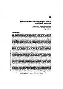
(2c) simple-2 vs constant-1.009: performance

(2d) simple-2 vs constant-1.009: ratios

(2e) 8 learners: performance

(2f) 8 learners: ratios

Figure 2. The figures on the left plot the performance over time. The learning curves display the average performance of each algorithm/portoflio over the epochs. The figures on the right show the ESBAS selection ratios over the epochs. Figures 2b and 2d also show the selection ratio standard deviation from one run to another. Nota bene: since the abscissæ are in epochs, all figure are actually logarithmic in meta-time. As a consequence, Epoch 12 is 1024 times larger than Epoch 2, and this explains for instance that simple-2 has actually a higher cumulative returns over the 12 epochs than simple.


Figure 2b reveals that the algorithm selection ratios are not very strong in favour of one or another at any time. Indeed, the variance in trajectory set collection makes simple better on some runs until the end. ESBAS proves to be efficient at selecting the best algorithm for each run and unexpectedly1 obtains a negative relative pseudo-regret of -90. More generally, Table 3 reveals that most of such two-fold portfolios with learning algorithms actually induced a strongly negative relative pseudo-regret. Figures 2c and 2d plot the typical curves obtained with ESBAS selecting from a portfolio constituted of a learning algorithm and an algorithm with a deterministic and stationary policy. ESBAS succeeds in remaining close to the best algorithm at each epoch. One can also observe a nice property: ESBAS even dominates both algorithm curves at some point, because the constant algorithm helps the learning algorithm to explore close to a reasonable policy. However, when the deterministic strategy is not so good, the reset of the stochastic bandits is harmful. As a result, learnerconstant portfolios may yield quite strong relative pseudoregrets: +169 in Figure 2c. However, when the constant algorithm expected return is over 1.13, slightly negative relative pseudo-regrets may still be obtained. Subsection 5.6 offers a straightforward improvement of ESBAS when one or several algorithm are known to be constant. ESBAS also performs well on larger portfolios of 8 learners (see Figure 2e) with negative relative pseudo-regrets: −10 (and −280 against the worst algorithm), even if the algorithms are, on average, almost selected uniformly as Figure 2f reveals. ESBAS offers some staggered learning, but more importantly, early bad policy accidents in learners are avoided. The same kind of results are obtained with 4-learner portfolios. If we add a constant algorithm to these larger portfolios, ESBAS behaviour is generally better than with the constant vs learner two-fold portfolios. 5.5. Reasons of ESBAS’s empirical success We interpret ESBAS’s success at reliably outperforming the best algorithm in the portfolio as the result of the four following potential added values: • Calibrated learning: ESBAS selects the algorithm that is the most fitted with the data size. This property allows for instance to use shallow algorithms when having only a few data and deep algorithms once collected a lot. • Diversified policies: ESBAS computes and experiments several policies. Those diversified policies generate trajectories that are less redundant, and therefore 1

It is unexpected because the ESBAS meta-algorithm does not intend to do better than the best algorithm in the portfolio: it simply tries to select it as much as possible.

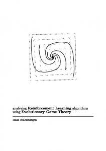
Figure 3. simple-2 vs constant-1.14 with no arm reset: performance

more informational. As a result, the policies trained on these trajectories should be more efficient. • Robustness: if one algorithm learns a terrible policy, it will soon be left apart until the next policy update. This property prevents the agent from repeating again and again the same blatant mistakes. • Run adaptation: obviously, there has to be an algorithm that is the best on average for one given task at one given meta-time. But depending on the variance in the trajectory collection, it is not necessarily the best one for each run. The ESBAS meta-algorithm tries and selects the algorithm that is the best at each run. All these properties are inherited by algorithm selection similarity with ensemble learning (Dietterich, 2002). Simply, instead of a vote amongst the algorithms to decide the control of the next transition (Wiering & Van Hasselt, 2008), ESBAS selects the best performing algorithm. In order to look deeper into the variance control effect of algorithm selection, in a similar fashion to ensemble learning, we tested two portfolios: four times the same algorithm n-2-simple, and four times the same algorithm n-3-simple. The results show that they both outperform the simple algorithm baseline, but only slightly (respectively −20 and −13). Our interpretation is that, in order to control variance, adding randomness is not as good as changing hypotheses, i.e. state space representations. 5.6. No arm reset for constant algorithms ESBAS’s worst results concern small portfolios of algorithms with constant policies. These ones do not improve over time and the full reset of the K-multi armed bandit urges ESBAS to explore again and again the same underachieving algorithm. One easy way to circumvent this drawback is to use the knowledge that these constant algorithms do not change and prevent their arm from resetting. By operating this way, when the learning algorithm(s) start(s)


outperforming the constant one, ESBAS simply neither exploits nor explores the constant algorithm anymore. Figure 3 displays the learning curve in the no-arm-reset configuration for the constant algorithm. One can notice that ESBAS’s learning curve follows perfectly the learning algorithm’s learning curve when this one outperforms the constant algorithm and achieves a strong negative relative pseudo-regret of -125. Still, when the constant algorithm does not perform as well as in Figure 3, another harmful phenomenon happens: the constant algorithm overrides the natural exploration of the learning algorithm in the early stages, and when the learning algorithm finally outperforms the constant algorithm, its exploration parameter is already low. This can be observed in experiments with constant algorithm of expected return inferior to 1, as reported in Table 3. 5.7. Assumptions transgressions Several results show that, in practice, the assumptions are transgressed. Firstly, Assumption 2, which states that more initial samples would necessarily help further learning convergence, is violated when the -greedy exploration parameter decreases with meta-time and not with the number of times this algorithm has been selected. Indeed, this is the main reason of the remaining mitigated results obtained in Subsection 5.6: instead of exploring in early stages, the agent selects the constant algorithm which results in generating over and over similar fair but non optimal trajectories. Finally, the learning algorithm might learn slower because of being decayed without having explored. Secondly, we also observe that Assumption 3 is transgressed. Indeed, it states that if a trajectory set is better than another for a given algorithm, then it’s the same for the other algorithms. This assumption does not prevent calibrated learning, but it prevents the run adaptation property introduced in Subsection 5.5 that states that an algorithm might be the best on some run and another one on other runs. Still, this assumption infringement does not seem to harm the experimental results. It even seems to help in general. Thirdly, off-policy reinforcement learning algorithms exist, but in practice, we use state space representations that distort their off-policy property (Munos et al., 2016). However, experiments do not reveal any obvious bias related to the off/on-policiness of the trajectory set the algorithms train on. And finally, let us recall here the unfairness of the exploration chosen by algorithms that has already been noticed in Subsection 3.4 and that also transgresses Assumption 3. Nevertheless, experiments did not raise any particular bias on this matter.

6. Related work Related to algorithm selection for RL, (Schweighofer & Doya, 2003) consists in using meta-learning to tune a fixed reinforcement algorithm in order to fit observed animal behaviour, which is a very different problem to ours. In (Cauwet et al., 2014; Liu & Teytaud, 2014), the reinforcement learning algorithm selection problem is solved with a portfolio composed of online RL algorithms. In those articles, the core problem is to balance the budget allocated to the sampling of old policies through a lag function, and budget allocated to the exploitation of the up-to-date algorithms. Their solution to the problem is thus independent from the reinforcement learning structure and has indeed been applied to a noisy optimisation solver selection (Cauwet et al., 2015). The main limitation from these works relies on the fact that on-policy algorithms were used, which prevents them from sharing trajectories among algorithms. Meta-learning specifically for the eligibility trace parameter has also been studied in (White & White, 2016). A recent work (Wang et al., 2016) studies the learning process of reinforcement learning algorithms and selects the best one for learning faster on a new task. This approach assumes several problem instances and is more related to the batch algorithm selection (see Section 3.1). AS for RL can also be related to ensemble RL. (Wiering & Van Hasselt, 2008) uses combinations of a set of RL algorithms to build its online control such as policy voting or value function averaging. This approach shows good results when all the algorithms are efficient, but not when some of them are underachieving. Hence, no convergence bound has been proven with this family of meta-algorithms. HORDE (Sutton et al., 2011) and multi-objective ensemble RL (Brys et al., 2014; van Seijen et al., 2016) are algorithms for hierarchical RL and do not directly compare with AS. Regarding policy selection, ESBAS advantageously compares √ with the RL with Policy Advice’s regret bounds of O( T log(T )) on static policies (Azar et al., 2013).

7. Conclusion In this article, we tackle the problem of selecting online offpolicy Reinforcement Learning algorithms. The problem is formalised as follows: from a fixed portfolio of algorithms, a meta-algorithm learns which one performs the best on the task at hand. Fairness of algorithm evaluation is granted by the fact that the RL algorithms learn off-policy. ESBAS, a novel meta-algorithm, is proposed. Its principle is to divide the meta-time scale into epochs. Algorithms are allowed to update their policies only at the start each epoch. As the policies are constant inside each epoch, the problem can be cast into a stochastic multi-armed bandit. An implementation with UCB1 is detailed and a theoretical analysis leads


to upper bounds on the short-sighted regret. The negotiation dialogue experiments show strong results: not only ESBAS succeeds in consistently selecting the best algorithm, but it also demonstrates its ability to perform staggered learning and to take advantage of the ensemble structure. The only mitigated results are obtained with algorithms that do not learn over time. A straightforward improvement of the ESBAS meta-algorithm is then proposed and its gain is observed on the task. As for next steps, we plan to work on an algorithm inspired by the lag principle introduced in (Cauwet et al., 2014), and apply it to our off-policy RL setting.


References Allesiardo, Robin and Féraud, Raphaël. Exp3 with drift detection for the switching bandit problem. In Proceedings of the 2nd IEEE International Conference on the Data Science and Advanced Analytics (DSAA), pp. 1–7. IEEE, 2015. Audibert, Jean-Yves and Bubeck, Sébastien. Best Arm Identification in Multi-Armed Bandits. In Proceedings of the 23th Conference on Learning Theory (COLT), Haifa, Israel, June 2010. Auer, Peter, Cesa-Bianchi, Nicolò, and Fischer, Paul. Finite-time analysis of the multiarmed bandit problem. Machine Learning, 2002a. doi: 10.1023/A:1013689704352. Auer, Peter, Cesa-Bianchi, Nicolo, Freund, Yoav, and Schapire, Robert E. The nonstochastic multiarmed bandit problem. SIAM Journal on Computing, 32(1):48–77, 2002b. Azar, Mohammad Gheshlaghi, Lazaric, Alessandro, and Brunskill, Emma. Regret bounds for reinforcement learning with policy advice. In Proceedings of the 23rd Joint European Conference on Machine Learning and Knowledge Discovery in Databases (ECML-PKDD), pp. 97–112. Springer, 2013. Azizzadenesheli, Kamyar, Lazaric, Alessandro, and Anandkumar, Animashree. Reinforcement learning of pomdps using spectral methods. In Proceedings of the 29th Annual Conference on Learning Theory (COLT), pp. 193–256, 2016. Böhmer, Wendelin, Springenberg, Jost Tobias, Boedecker, Joschka, Riedmiller, Martin, and Obermayer, Klaus. Autonomous learning of state representations for control: An emerging field aims to autonomously learn state representations for reinforcement learning agents from their real-world sensor observations. KIKünstliche Intelligenz, 2015. Brys, Tim, Taylor, Matthew E, and Nowé, Ann. Using ensemble techniques and multi-objectivization to solve reinforcement learning problems. In Proceedings of the 21st European Conference on Artificial Intelligence (ECAI), pp. 981–982. IOS Press, 2014. Brys, Tim, Harutyunyan, Anna, Suay, Halit Bener, Chernova, Sonia, Taylor, Matthew E, and Nowé, Ann. Reinforcement learning from demonstration through shaping. In Proceedings of the 24th International Joint Conference on Artificial Intelligence (IJCAI), 2015. Bubeck, Sébastien and Cesa-Bianchi, Nicolò. Regret analysis of stochastic and nonstochastic multi-armed bandit problems. Foundations and Trends in Machine Learning, 2012. doi: 10. 1561/2200000024. Cauwet, Marie-Liesse, Liu, Jialin, and Teytaud, Olivier. Algorithm portfolios for noisy optimization: Compare solvers early. In Learning and Intelligent Optimization. Springer, 2014. Cauwet, Marie-Liesse, Liu, Jialin, Rozière, Baptiste, and Teytaud, Olivier. Algorithm Portfolios for Noisy Optimization. ArXiv e-prints, November 2015. Dietterich, Thomas G. Ensemble learning. The handbook of brain theory and neural networks, 2:110–125, 2002.

El Asri, Layla, Laroche, Romain, and Pietquin, Olivier. Compact and interpretable dialogue state representation with genetic sparse distributed memory. In Proceedings of the 7th International Workshop on Spoken Dialogue Systems (IWSDS), Finland, January 2016. Ernst, Damien, Geurts, Pierre, and Wehenkel, Louis. Tree-based batch mode reinforcement learning. Journal of Machine Learning Research, 2005. Even-Dar, Eyal, Mannor, Shie, and Mansour, Yishay. Pac bounds for multi-armed bandit and markov decision processes. In Computational Learning Theory. Springer, 2002. Fatemi, Mehdi, El Asri, Layla, Schulz, Hannes, He, Jing, and Suleman, Kaheer. Policy networks with two-stage training for dialogue systems. arXiv preprint arXiv:1606.03152, 2016. Fialho, Álvaro, Da Costa, Luis, Schoenauer, Marc, and Sebag, Michele. Analyzing bandit-based adaptive operator selection mechanisms. Annals of Mathematics and Artificial Intelligence, 2010. Frampton, Matthew and Lemon, Oliver. Learning more effective dialogue strategies using limited dialogue move features. In Proceedings of the 21st International Conference on Computational Linguistics and the 44th annual meeting of the Association for Computational Linguistics (ACL), pp. 185–192. Association for Computational Linguistics, 2006. Gagliolo, Matteo and Schmidhuber, Jürgen. Learning dynamic algorithm portfolios. Annals of Mathematics and Artificial Intelligence, 2006. Gagliolo, Matteo and Schmidhuber, Jürgen. Algorithm selection as a bandit problem with unbounded losses. In Learning and Intelligent Optimization. Springer, 2010. Garivier, A. and Moulines, E. On Upper-Confidence Bound Policies for Non-Stationary Bandit Problems. ArXiv e-prints, May 2008. Gaši´c, M, Jurˇcíˇcek, F, Keizer, Simon, Mairesse, François, Thomson, Blaise, Yu, Kai, and Young, Steve. Gaussian processes for fast policy optimisation of pomdp-based dialogue managers. In Proceedings of the 11th Annual Meeting of the Special Interest Group on Discourse and Dialogue (Sigdial), pp. 201–204. Association for Computational Linguistics, 2010. Geist, Matthieu and Pietquin, Olivier. Kalman temporal differences. Journal of Artificial Intelligence Research, 2010. Genevay, Aude and Laroche, Romain. Transfer learning for user adaptation in spoken dialogue systems. In Proceedings of the 15th International Conference on Autonomous Agents and Multi-Agent Systems (AAMAS). International Foundation for Autonomous Agents and Multiagent Systems, 2016. Gomes, Carla P. and Selman, Bart. Algorithm portfolios. Artificial Intelligence, 2001. ISSN 0004-3702. doi: http://dx.doi.org/ 10.1016/S0004-3702(00)00081-3. Tradeoffs under Bounded Resources. Khouzaimi, Hatim, Laroche, Romain, and Lefevre, Fabrice. Optimising turn-taking strategies with reinforcement learning. In Proceedings of the 16th Annual Meeting of the Special Interest Group on Discourse and Dialogue (Sigdial), 2015.

Algorithm selection of off-policy reinforcement learning algorithms Kotthoff, Lars. Algorithm selection for combinatorial search problems: A survey. arXiv preprint arXiv:1210.7959, 2012. Laroche, Romain and Genevay, Aude. A negotiation dialogue game. In Proceedings of the 7th International Workshop on Spoken Dialogue Systems (IWSDS), Finland, 2016. Laroche, Romain, Putois, Ghislain, Bretier, Philippe, and BouchonMeunier, Bernadette. Hybridisation of expertise and reinforcement learning in dialogue systems. In Proceedings of the 9th Annual Conference of the International Speech Communication Association (Interspeech), 2009. Legenstein, Robert, Wilbert, Niko, and Wiskott, Laurenz. Reinforcement learning on slow features of high-dimensional input streams. PLoS Computational Biology, 2010. Levin, Esther and Pieraccini, Roberto. A stochastic model of computer-human interaction for learning dialogue strategies. In Proceedings of the 5th European Conference on Speech Communication and Technology (Eurospeech), 1997. Liu, Jialin and Teytaud, Olivier. Meta online learning: experiments on a unit commitment problem. In Proceedings of the 22nd European Symposium on Artificial Neural Networks, Computational Intelligence and Machine Learning (ESANN), 2014. Lovejoy, William S. Computationally feasible bounds for partially observed markov decision processes. Operational Research, 1991. Maei, Hamid R, Szepesvári, Csaba, Bhatnagar, Shalabh, and Sutton, Richard S. Toward off-policy learning control with function approximation. In Proceedings of the 27th International Conference on Machine Learning (ICML-10), pp. 719–726, 2010. Mnih, Volodymyr, Kavukcuoglu, Koray, Silver, David, Graves, Alex, Antonoglou, Ioannis, Wierstra, Daan, and Riedmiller, Martin. Playing atari with deep reinforcement learning. arXiv preprint arXiv:1312.5602, 2013. Munos, Rémi, Stepleton, Tom, Harutyunyan, Anna, and Bellemare, Marc G. Safe and efficient off-policy reinforcement learning. CoRR, abs/1606.02647, 2016. Ng, Andrew Y and Jordan, Michael. Pegasus: A policy search method for large mdps and pomdps. In Proceedings of the Sixteenth conference on Uncertainty in artificial intelligence, pp. 406–415. Morgan Kaufmann Publishers Inc., 2000. Perchet, Vianney and Rigollet, Philippe. The multi-armed bandit problem with covariates. The Annals of Statistics, 2013. Pietquin, Olivier, Geist, Matthieu, and Chandramohan, Senthilkumar. Sample efficient on-line learning of optimal dialogue policies with kalman temporal differences. In Proceedings of the 22nd International Joint Conference on Artificial Intelligence (IJCAI), 2011.

Silver, David, Huang, Aja, Maddison, Chris J., Guez, Arthur, Sifre, Laurent, van den Driessche, George, Schrittwieser, Julian, Antonoglou, Ioannis, Panneershelvam, Veda, Lanctot, Marc, et al. Mastering the game of go with deep neural networks and tree search. Nature, 2016. Singh, Satinder P., Kearns, Michael J., Litman, Diane J., and Walker, Marilyn A. Reinforcement learning for spoken dialogue systems. In Proceedings of the 13th Annual Conference on Neural Information Processing Systems (NIPS), 1999. Smith-Miles, Kate A. Cross-disciplinary perspectives on metalearning for algorithm selection. ACM Computational Survey, 2009. Sutton, Richard S. and Barto, Andrew G. Reinforcement Learning: An Introduction (Adaptive Computation and Machine Learning). The MIT Press, March 1998. ISBN 0262193981. Sutton, Richard S, Modayil, Joseph, Delp, Michael, Degris, Thomas, Pilarski, Patrick M, White, Adam, and Precup, Doina. Horde: A scalable real-time architecture for learning knowledge from unsupervised sensorimotor interaction. In Proceedings of the 10th International Conference on Autonomous Agents and Multi-Agent Systems (AAMAS), pp. 761–768. International Foundation for Autonomous Agents and Multiagent Systems, 2011. van Seijen, Harm, Fatemi, Mehdi, and Romoff, Joshua. Improving scalability of reinforcement learning by separation of concerns. arXiv preprint arXiv:1612.05159, 2016. Walker, Marilyn A, Fromer, Jeanne C, and Narayanan, Shrikanth. Learning optimal dialogue strategies: A case study of a spoken dialogue agent for email. In Proceedings of the 36th Annual Meeting of the Association for Computational Linguistics and 17th International Conference on Computational LinguisticsVolume 2, pp. 1345–1351. Association for Computational Linguistics, 1998. Wang, Jane X., Kurth-Nelson, Zeb, Tirumala, Dhruva, Soyer, Hubert, Leibo, Joel Z., Munos, Rémi, Blundell, Charles, Kumaran, Dharshan, and Botvinick, Matt. Learning to reinforcement learn. CoRR, abs/1611.05763, 2016. Watkins, C.J.C.H. Learning from Delayed Rewards. PhD thesis, Cambridge University, Cambridge (England), May 1989. White, Martha and White, Adam. Adapting the trace parameter in reinforcement learning. In Proceedings of the 15th International Conference on Autonomous Agents and Multi-Agent Systems (AAMAS). International Foundation for Autonomous Agents and Multiagent Systems, 2016. Wiering, Marco A and Van Hasselt, Hado. Ensemble algorithms in reinforcement learning. IEEE Transactions on Systems, Man, and Cybernetics, Part B (Cybernetics), 38(4):930–936, 2008.

Rice, John R. The algorithm selection problem. Advances in Computers, 1976.

Williams, Jason, Raux, Antoine, and Henderson, Matthew. The dialog state tracking challenge series: A review. Dialogue & Discourse, 7(3):4–33, 2016.

Riedmiller, Martin. Neural Fitted-Q Iteration – first experiences with a data efficient neural reinforcement learning method. In Machine Learning: ECML 2005. Springer, 2005.

Xu, Lin, Hutter, Frank, Hoos, Holger H, and Leyton-Brown, Kevin. Satzilla: portfolio-based algorithm selection for sat. Journal of Artificial Intelligence Research, 2008.

Schweighofer, Nicolas and Doya, Kenji. Meta-learning in reinforcement learning. Neural Networks, 2003.


A. Glossary Symbol t τ, T a(t) o(t) R(t) A Ω Rmin Rmax ετ |X| Ja, bK E γ µ(ετ ) DT ετ (t) π π∗ α E+ α SD Φα D α πD I P Ψ K σ σ(τ ) Ex0 [f (x0 )] Eµα D P(x|y) Eµ∗∞ σα ρσabs (T ) ρσrel (T ) O(f (x)) κ Ξ β ξ ρσss (T ) ∆ † ∆†β bxc σ ESBAS Θ(f (x)) σ∗

Designation Reinforcement learning time aka RL-time Meta-algorithm time aka meta-time Action taken at RL-time t Observation made at RL-time t Reward received at RL-time t Action set Observation set Lower bound of values taken by R(t) Upper bound of values taken by R(t) Trajectory collected at meta-time τ Size of finite set/list/collection X Ensemble of integers comprised between a and b Space of trajectories Discount factor of the decision process Return of trajectory ετ aka objective function Trajectory set collected until meta-time T History of ετ until RL-time t Policy Optimal policy Algorithm Ensemble of trajectory sets State space of algorithm α from trajectory set D State space projection of algorithm α from trajectory set D Policy learnt by algorithm α from trajectory set D Problem instance set Algorithm set aka portfolio Features characterising problem instances Size of the portfolio Meta-algorithm Algorithm selected by meta-algorithm σ at meta-time τ Expected value of f (x) conditionally to x = x0 α Expected return of trajectories controlled by policy πD Probability that X = x conditionally to Y = y Optimal expected return Canonical meta-algorithm exclusively selecting algorithm α Absolute pseudo-regret Relative pseudo-regret Set of functions that get asymptotically dominated by κf (x) Constant number Stochastic K-armed bandit algorithm Epoch index Parameter of the UCB algorithm Short-sighted pseudo-regret Gap between the best arm and another arm Index of the second best algorithm Gap of the second best arm at epoch β Rounding of x at the closest integer below The ESBAS meta-algorithm Set of functions asymptotically dominating κf (x) and dominated by κ0 f (x) Best meta-algorithm among the canonical ones

First use Section 2 Section 2 Figure 1 Figure 1 Figure 1 Section 2 Section 2 Section 2 Section 2 Equation 2.1 Equation 2.1 Equation 2.1 Equation 2.1 Equation 2.2 Equation 2.2 Equation 2.4 Equation 2.5 Section 2 Section 2 Equation 2.6 Equation 2.6 Equation 2.7 Equation 2.7 Section 2 Section 3.1 Section 3.1 Section 3.1 Section 3.2 Equation 3.1 Section 3.2 Equation 3.2 Equation 3.2 Equation 3.3a Equation 3.4 Section 3.3 Definition 1 Definition 2 Section 4 Theorem 3 Section 4.1 Section 4.1 Pseudo-code 2 Definition 3 Theorem 2 Theorem 2 Theorem 2 Theorem 2 Theorem 2 Table 1 Theorem 3


Symbol p, ps , pu η νηp U[a, b] sf Rps (sf ) R EF P ROP(η) A SK R EPEAT ACCEPT(η) E ND D IAL SERsu scoreasr N (x, v) R EF I NSIST R EF N EW P ROP ACCEPT β Φα φ0 φasr φdif φt φnoise simple fast simple-2 fast-2 n-1-simple n-1-fast n-1-simple-2 n-1-fast-2 constant-µ ζ

Designation Player, system player, and (simulated) user player Option to agree or disagree on Cost of booking/selecting option ν for player p Uniform distribution between a and b Final state reached in a trajectory Immediate reward received by the system player at the end of the dialogue Dialogue act consisting in proposing option η Dialogue act consisting in asking the other player to repeat what he said Dialogue act consisting in accepting proposition η Dialogue act consisting in ending the dialogue Sentence error rate of system ps listening to user pu Speech recognition score Normal distribution of centre x and variance v 2 R EF P ROP(η), with η being the last proposed option R EF P ROP(η), with η being the best option that has not been proposed yet ACCEPT(η), with η being the last understood option proposition -greedy exploration in function of epoch β Set of features of algorithm α Constant feature: always equal to 1 α ASR feature: equal to the last recognition score Cost feature: equal to the difference of cost of proposed and targeted options RL-time feature Noise feature FQI with Φ = {φ0 , φasr , φdif , φt } FQI with Φ = {φ0 , φasr , φdif } FQI with Φ = {φ0 , φasr , φdif , φt , φasr φdif , φt φasr , φdif φt , φ2asr , φ2dif , φ2t } FQI with Φ = {φ0 , φasr , φdif , φasr φdif , φ2asr , φ2dif } FQI with Φ = {φ0 , φasr , φdif , φt , φnoise } FQI with Φ = {φ0 , φasr , φdif , φnoise } FQI with Φ = {φ0 , φasr , φdif , φt , φnoise , φasr φdif , φt φnoise , φasr φt , φdif φnoise , φasr φnoise , φdif φt , φ2asr , φ2dif , φ2t , φ2noise } FQI with Φ = {φ0 , φasr , φdif , φt } Non-learning algorithm with average performance µ Number of noisy features added to the feature set

First use Section 5.1 Section 5.1 Section 5.1 Section 5.1 Equation 5.1 Equation 5.1 Section 5.1 Section 5.1 Section 5.1 Section 5.1 Section 5.2 Equation 5.4 Equation 5.4 Section 5.2 Section 5.2 Section 5.2 Section 5.3 Section 5.3 Section 5.3 Section 5.3 Section 5.3 Section 5.3 Section 5.3 Section 5.3 Section 5.3 Section 5.3 Section 5.3 Section 5.3 Section 5.3 Section 5.3 Section 5.3 Section 5.3 Section 5.3


B. Recall of definitions and assumptions B.1. Defitions Definition 1 (Absolute pseudo-regret). The absolute pseudo-regret ρσabs (T ) compares the meta-algorithm’s expected return with the optimal expected return: " T # X σ(τ ) σ ∗ ρabs (T ) = T Eµ∞ − Eσ EµDσ . (3.5) τ −1

τ =1

Definition 2 (Relative pseudo-regret). The relative pseudo-regret ρσrel (T ) compares the σ meta-algorithm’s expected return with the expected return of the best canonical meta-algorithm: " ρσrel (T )

= max Eσα α∈P

T X τ =1

# Eµα σα Dτ −1

" − Eσ

T X

# σ(τ ) EµDσ τ −1

.

(3.6)

τ =1

Definition 3 (Short-sighted pseudo-regret). The short-sighted pseudo-regret ρσss (T ) is the difference between the immediate best expected return algorithm and the one selected: " ρσss (T )

= Eσ

T X

τ =1

σ max Eµα Dτ −1 α∈P

−

σ(τ ) EµDσ τ −1

# .

(4.1)

B.2. Assumptions Assumption 1 (More data is better data). The algorithms produce better policies with a larger trajectory set on average, whatever the algorithm that controlled the additional trajectory: α ∀D ∈ E + , ∀α, α0 ∈ P, Eµα (3.8) D ≤ Eα0 EµD∪εα0 . Assumption 2 (Order compatibility). If an algorithm produces a better policy with one trajectory set than with another, then it remains the same, on average, after collecting an additional trajectory from any algorithm: ∀D, D0 ∈ E + , ∀α, α0 ∈ P, α α α Eµα D < EµD 0 ⇒ Eα0 EµD∪εα0 ≤ Eα0 EµD 0 ∪εα0 .

(3.9)

Assumption 3 (Learning is fair). If one trajectory set is better than another for one given algorithm, it is the same for other algorithms. ∀α, α0 ∈ P, ∀D, D0 ∈ E + , 0

0

α α α Eµα D < EµD 0 ⇒ EµD ≤ EµD 0 .

(3.11)


C. Not worse than the worst Theorem 1 (Not worse than the worst). The absolute pseudo-regret is bounded by the worst algorithm absolute pseudo-regret in order of magnitude: α

ρσabs (T ) ∈ O max ρσabs (T ) .

∀σ,

(3.10)

α∈P

Proof. From Definition 1:

" ρσabs (T )

=

T Eµ∗∞

− Eσ

T X

# σ(τ ) EµDσ τ −1

,

(C.1a)

τ =1

 ρσabs (T )

=

T Eµ∗∞

X

−

σ |subα (DT )|

X

Eσ 

σ |subα (DT )|

 =

X

(C.1b)

i

i=1

α∈P

ρσabs (T )

 , σ Eµα Dτ α −1

Eσ |sub

α

(DTσ )|Eµ∗∞

−

X

 , σ Eµα Dτ α −1

(C.1c)

i

i=1

α∈P

where subα (D) is the subset of D with all the trajectories generated with algorithm α, where τiα is the index of the ith trajectory generated with algorithm α, and where |S| is the cardinality of finite set S. By convention, let us state that Eµα = Eµ∗∞ if |subα (DTσ )|< i. D σα τ −1 i

Then: ρσabs (T ) =

T XX

Eσ Eµ∗∞ − Eµα D σα

τ −1 i

α∈P i=1

.

(C.2)

To conclude, let us prove by mathematical induction the following inequality: Eσ Eµα D σα

τ −1 i

h i α ≥ Eσα Eµα Dσ i−1

is true by vacuity for i = 0: both left and right terms equal Eµα ∅ . Now let us assume the property true for i and prove it for i + 1: Eσ

σ Eµα Dτ α

i+1

Eσ

σ Eµα Dτ α

i+1

α

= Eσ

−1

#

"

Eµ σ σ Dτ α −1 ∪εα ∪ Dτ α i

Eσ

σ Eµα Dτ α

i+1

−1

σ \Dτ α

,

,

α −1 Sτi+1 σ σ(τ ) α Dτ α −1 ∪ε ∪ τ =τ α +1 ε

(C.3b)

i

" = Eσ Eµ

(C.3a)

i

# i

−1

" = Eσ Eµ

−1

i+1

# α −τ α −1 Sτi+1 σ(τ α +τ ) i σ α i ε Dτ α −1 ∪ε ∪ τ =1

.

(C.3c)

i

If |subα (DTσ )|≥ i + 1, by applying mathematical induction assumption, then by applying Assumption 2 and finally by applying Assumption 1 recursively, we infer that: h i α α σ Eσ EµD α ≥ Eσα Eµα , (C.4a) Dσ τ

i

−1

i−1

Eσ Eµα D σα

∪εα τ −1 i

Eσ Eµα D σα τ

i

α i−1 ∪ε

−1

∪εα

h α ≥ Eσα Eµα Dσ

h i α , ≥ Eσα Eµα Dσ i

i

,

(C.4b) (C.4c)

Algorithm selection of off-policy reinforcement learning algorithms " # h i α −τ α −1 α . Eσ Eµ σ ≥ Eσα Eµα Sτi+1 Dσ σ(τ α +τ ) i Dτ α −1 ∪εα ∪ τ =1

ε

i

i

(C.4d)

i

If |subα (DTσ )|< i + 1, the same inequality is straightforwardly obtained, since, by convention EµkD

τk i+1

= Eµ∗∞ , and since, by definition

∀D ∈ E + , ∀α ∈ P, Eµ∗∞ ≥ Eµα D. The mathematical induction proof is complete. This result leads to the following inequalities:

ρσabs (T ) ≤

T XX

i h α , Eσα Eµ∗∞ − Eµα σ D i−1

α∈P i=1

ρσabs (T ) ≤

X

α

ρσabs (T ) ,

(C.5a)

(C.5b)

α∈P

α

ρσabs (T ) ≤ K max ρσabs (T ) , α∈P

(C.5c)

which leads directly to the result: ∀σ,

ρσabs (T ) ∈ O

k max ρσabs (T ) .

αk ∈P

(C.6)

This proof may seem to the reader rather complex for such an intuitive and loose result but algorithm selection σ and the algorithms it selects may act tricky. For instance selecting algorithm α only when the collected trajectory sets contains misleading examples (i.e. with worse expected return than with an empty trajectory set) implies that the following unintuitive inequality is always true: α σ α . In order to control all the possible outcomes, one needs to translate the selections of algorithm α into σ ’s view. Eµα ≤ Eµα Dτ Dσ −1 τ −1


D. ESBAS short-sighted pseudo-regret upper order of magnitude Theorem 2 (ESBAS short-sighted pseudo-regret). If the stochastic multi-armed bandit Ξ guarantees a regret of order of magnitude O(log(T )/∆†β ), then:   blog(T )c X ESBAS β . ρσss (T ) ∈ O  (4.4) ∆†β β=0 α Proof. By simplification of notation, Eµα Dβ = EµD σ ESBAS . From Definition 3: 2β −1

" ESBAS

ρσss

(T ) = Eσ ESBAS

# T X σ ESBAS (τ ) ESBAS max Eµα − Eµ , σ ESBAS Dσ α∈P

τ =1

" ESBAS ρσss (T )

= Eσ ESBAS

(D.1a)

Dτ −1

τ −1

# T X σ ESBAS (τ ) α , max Eµβτ − Eµβτ

(D.1b)

α∈P

τ =1

 ESBAS ρσss (T )

ESBAS

ρσss

blog2 (T )c 2β+1 −1

≤ Eσ ESBAS 

blog2 (T )c

(T ) ≤

X

X

X

β=0

τ =2β

ESBAS

ρσss

max Eµα β α∈P

−

σ ESBAS (τ ) Eµβ

 ,

(D.1c)

(β),

(D.1d)

β=0

ESBAS

where βτ is the epoch of meta-time τ . A bound on short-sighted pseudo-regret ρσss stochastic bandit Ξ regret bounds in O (log(T )/∆):

(β) for each epoch β can then be obtained by the

 ESBAS ρσss (β)

2β+1 X−1

= Eσ ESBAS 

τ =2β

ESBAS ρσss (β)

ESBAS ρσss (β)

⇔ ∃κ1 > 0,

ESBAS

ρσss

where

and where

(β) ≤

−

σ ESBAS (τ ) Eµβ

 ,

(D.2a)

! log(2β ) , ∆β

∈O

∈O

max Eµα β α∈P

β ∆β

(D.2b)

,

(D.2c)

κ1 β , ∆β

(D.2d)

X 1 1 = ∆β α∈P ∆α β

∆α β =

(D.2e)

   +∞

α if Eµα β = maxα0 ∈P Eµβ ,

0  α  maxα0 ∈P Eµα β − Eµβ

otherwise.

0

Since we are interested in the order of magnitude, we can once again only consider the upper bound of [ 1 ∈ O ∆β α∈P

1 ∆α β

1 ∆β

(D.2f)

:

! ,

(D.3a)

Algorithm selection of off-policy reinforcement learning algorithms ! 1 1 ∈ O max α , α∈P ∆ ∆β β 1 κ2 ≤ †, ∆β ∆β

⇔ ∃κ2 > 0,

(D.3b)

(D.3c)

where the second best algorithm at epoch β such that ∆†β > 0 is noted αβ† . Injected in Equation D.1d, it becomes: ESBAS

ρσss

blog2 (T )c

(T ) ≤ κ1 κ2

X

β

β=0

∆†β

,

(D.4)

which proves the result.

D.1. Corollaries of Theorem 2 Corollary 1. If

∆†β

∈ Θ (1), then

ESBAS ρσss (T )

log2 (T )

∈O

∆†∞

! , where ∆†∞ = µ∗∞ − µ†∞ > 0.

Proof. ∆†β ∈ Ω (1) means that only one algorithm α∗ converges to the optimal asymptotic performance µ∗∞ and that ∃∆†∞ = µ∗∞ −µ†∞ > 0 such that ∀2 > 0, ∃β1 ∈ N, such that ∀β ≥ β1 , ∆†β > ∆†∞ − . In this case, the following bound can be deduced from equation D.4: blog(T )c ESBAS

ρσss

X

(T ) ≤ κ4 +

β=β1

ESBAS

ρσss

κ1 κ2 ∆†∞ −

κ1 κ2 log2 (T )

(T ) ≤ κ4 +

2(∆†∞ − )

β,

,

(D.5a)

(D.5b)

where κ4 is a constant equal to the short-sighted pseudo-regret before epoch β1 : ESBAS

κ4 = ρσss

2β1 −1

(D.6)

Equation D.5b directly leads to the corollary. † ESBAS † Corollary 2. If ∆†β ∈ Θ β −m , then ρσss (T ) ∈ O logm +2 (T ) . Proof. If ∆†β decreases slower than polynomially in epochs, which implies decreasing polylogarithmically in meta-time, i.e. ∃κ5 > †

0, ∃m† > 0, ∃β2 ∈ N, such that ∀β ≥ β2 , ∆†β > κ5 β −m , then, from Equation D.4: blog(T )c ESBAS

ρσss

X

(T ) ≤ κ6 +

β=β2 blog(T )c ESBAS

ρσss

X

(T ) ≤ κ6 +

β=β2

ESBAS

ρσss

(T ) ≤

κ1 κ2 β, κ5 β −m†

(D.7a)

κ1 κ2 m† +1 β , κ5

(D.7b)

† κ1 κ2 logm +2 (T ), κ5

(D.7c)


κ6 = ρσss Equation D.7c directly leads to the corollary.

2β2 −1 .

(D.8)

Algorithm selection of off-policy reinforcement learning algorithms † † ESBAS Corollary 3. If ∆†β ∈ Θ T −c , then ρσss (T ) ∈ O T c log(T ) .

Proof. If ∆†β decreases slower than a fractional power of meta-time T , then ∃κ7 > 0, 0 < c† < 1, ∃β3 ∈ N, such that ∀β ≥ β3 , †

∆†β > κ7 T −c , and therefore, from Equation D.4: blog(T )c ESBAS

ρσss

X

(T ) ≤ κ8 +

β=β3

blog(T )c ESBAS

ρσss

X

(T ) ≤ κ8 +

blog(T )c ESBAS

(D.9a)

κ1 κ2 †

β=β3

ρσss

κ1 κ2 β, κ7 τ −c†

(T ) ≤ κ8 +

X β=β3

κ7 (2β )−c

β,

κ1 κ2 c† β , β 2 κ7

(D.9b)

(D.9c)


κ8 = ρσss

2β3 −1 .

(D.10)

The sum in Equation D.9c is solved as follows: n X i =i0 n X

ixi−1 ,

ixi = x

n X d xi , dx i=i

ixi = x

d

P n

i=i0

d i

i =i0

,

xn+1 − xi0 x−1

ix = x

ixi =

xi

dx

dx

i =i0 n X

(D.11b)

0

i =i0

n X

(D.11a)

i=i0

i =i0

n X

n X

ixi = x

(D.11c)

! ,

(D.11d)

x (x − 1)nxn − xn − (x − 1)i0 xi0 −1 + xi0 . 2 (x − 1)

(D.11e)

This result, injected in Equation D.9c, induces that ∀3 > 0, ∃T1 ∈ N, ∀T ≥ T1 : †

ESBAS ρσss (T )

† κ1 κ2 (1 + 0 )2c ≤ κ8 + log(T )2c log(T ) , κ7 (2c† − 1)

(D.12a)

†

ESBAS

ρσss

which proves the corollary.

(T ) ≤ κ8 +

κ1 κ2 (1 + 0 )2c c† T log(T ), κ7 (2c† − 1)

(D.12b)


E. ESBAS abolute pseudo-regret bound Theorem 3 (ESBAS absolute pseudo-regret upper bound). If the stochastic multi-armed bandit Ξ guarantees that the best arm has been selected in the T first episodes at least T /K times, with high probability δT ∈ O(1/T ), then: ∃κ > 0, ∀T ≥ 9K 2 , ∗

ESBAS

ρσabs (T ) ≤ (3K + 1)ρσabs ESBAS

+ρσss

T 3K

(4.5)

(T ) + κ log(T ). α

where algorithm selection σ ∗ selects exclusively algorithm α∗ = argminα∈P ρσabs (T ). ESBAS

Proof. The ESBAS absolute pseudo-regret is written with the following notation simplifications : Dτ −1 = Dτσ−1 and kτ = σ ESBAS (τ ): " ESBAS ρσabs (T )

=

T Eµ∗∞

− Eσ ESBAS

T X

# Eµ

τ =1

" ESBAS ρσabs (T )

=

T Eµ∗∞

− Eσ ESBAS

T X

σ ESBAS (τ ) ESBAS

σ Dτ −1

,

(E.1a)

# EµkDττ −1

.

(E.1b)

τ =1

Let σ ∗ denote the algorithm selection selecting exclusively α∗ , and α∗ be the algorithm minimising the algorithm absolute pseudo-regret: k

α∗ = argmin ρσabs (T ).

(E.2)

αk ∈P

Note that σ ∗ is the optimal constant algorithm selection at horizon T , but it is not necessarily the optimal algorithm selection: there might exist, and there probably exists a non constant algorithm selection yielding a smaller pseudo-regret. ESBAS

The ESBAS absolute pseudo-regret ρσabs (T ) can be decomposed into the pseudo-regret for not having followed the optimal constant algorithm selection σ ∗ and the pseudo-regret for not having selected the algorithm with the highest return, i.e. between the pseudo-regret on the trajectory and the pseudo-regret on the immediate optimal return: " ESBAS ρσabs (T )

=

T Eµ∗∞

− Eσ ESBAS

T X

# Eµ∗sub∗ (Dτ −1 )

" + Eσ ESBAS

τ =1

T X

# Eµ∗sub∗ (Dτ −1 )

" − Eσ ESBAS

τ =1

T X

# EµkDττ −1

,

(E.3)

τ =1

where Eµ∗sub∗ (D

∗ ∗ ∗ ) is the expected return of policy πsub∗ (Dτ −1 ) , learnt by algorithm α on trajectory set sub (Dτ −1 ), which is the trajectory subset of Dτ −1 obtained by removing all trajectories that were not generated with algorithm α∗ . τ −1

First line of Equation E.3 can be rewritten as follows: " T Eµ∗∞

− Eσ ESBAS

T X

# Eµ∗sub∗ (Dτ −1 )

=

τ =1

T X

h i Eµ∗∞ − Eσ ESBAS Eµ∗sub∗ (Dτ −1 ) .

(E.4)

τ =1

The key point in Equation E.4 is to evaluate the size of sub∗ (Dτ −1 ). On the one side, Assumption 3 of fairness states that one algorithm learns as fast as any another over any history. The asymptotically optimal algorithm(s) when τ → ∞ is(are) therefore the same one(s) whatever the the algorithm selection is. On the other side, let 1 − δτ denote the probability, that at time τ , the following inequality is true: |sub∗ (Dτ −1 ) |≥

τ −1 . 3K

(E.5)

With probability δτ , inequality E.5 is not guaranteed and nothing can be inferred about Eµ∗sub∗ (D Rmin /(1 − γ). Let follows:

τ −1 E3K

be the subset of E

τ −1

such that ∀D ∈ δτ =

τ −1 E3K , |sub∗ (D)|≥

X τ −1 D∈E τ −1 \E3K

P(D|σ ESBAS ).

) , except it is bounded under by b(τ − 1)/3Kc. Then, δτ can be expressed as τ −1

(E.6)

Algorithm selection of off-policy reinforcement learning algorithms With these new notations: i h Eµ∗∞ − Eσ ESBAS Eµ∗sub∗ (Dτ −1 ) ≤ Eµ∗∞ −

X

Rmin , 1−γ

P(D|σ ESBAS )Eµ∗sub∗ (D) − δτ

τ −1 D∈E3K

i h Eµ∗∞ − Eσ ESBAS Eµ∗sub∗ (Dτ −1 ) ≤ (1 − δτ )Eµ∗∞ −

X

P(D|σ ESBAS )Eµ∗sub∗ (D) + δτ

(E.7a)

Eµ∗∞ −

τ −1 D∈E3K

Rmin . 1−γ

(E.7b)

Let consider E ∗ (α, N ) the set of all sets D such that |subα (D)|= N and such that last trajectory in D was generated by α. Since ESBAS, with Ξ, a stochastic bandit with regret in O(log(T )/∆), guarantees that all algorithms will eventually be selected an infinity of times, we know that : X ∀α ∈ P, ∀N ∈ N, P(D|σ ESBAS ) = 1. (E.8) D ∈E + (α,N )

By applying recursively Assumption 2, one demonstrates that: X

P(D|σ ESBAS )Eµα subα (D) ≥

D ∈E + (α,N )

X

X

P(D|σ α )Eµα D,

(E.9a)

D∈E N

h i α P(D|σ ESBAS )Eµα subα (D) ≥ Eσ α EµD σα .

(E.9b)

N

D ∈E + (α,N )

One also notices the following piece-wisely domination from applying recursively Assumption 1: X

(1 − δτ )Eµ∗∞ −

τ −1 D ∈E3K

X

(1 − δτ )Eµ∗∞ −

X

P(D|σ ESBAS )Eµ∗sub∗ (D) ≤

X

P(D|σ ESBAS ) Eµ∗∞ − Eµ∗sub∗ (D) , (E.10b)

X

P(D|σ ESBAS )Eµ∗sub∗ (D) ≤

X

(E.10a)

−1 c)&|D|≤τ −1 D∈E + (α∗ ,b τ3K

τ −1 D ∈E3K

(1 − δτ )Eµ∗∞ −

P(D|σ ESBAS ) Eµ∗∞ − Eµ∗sub∗ (D) ,

τ −1 D∈E3K

τ −1 D ∈E3K

(1 − δτ )Eµ∗∞ −

X

P(D|σ ESBAS )Eµ∗sub∗ (D) =

P(D|σ ESBAS ) Eµ∗∞ − Eµ∗sub∗ (D) ,

(E.10c)

−1 c) D∈E + (α∗ ,b τ3K

X

P(D|σ ESBAS )Eµ∗sub∗ (D) ≤ Eµ∗∞ −

τ −1 D ∈E3K

P(D|σ ESBAS )Eµ∗sub∗ (D) .

(E.10d)

−1 D∈E + (α∗ ,b τ3K c)

Then, by applying results from Equations E.9b and E.10d into Equation E.7b, one obtains:  Eµ∗∞

− Eσ ESBAS

h

Eµ∗sub∗ (Dτ −1 )

i

≤

Eµ∗∞

−



Eσ∗ Eµα σ∗ D

τ −1 3K

 + δτ

Eµ∗∞ −

Rmin . 1−γ

(E.11)

Next, the terms in the first line of Equation E.3 are bounded as follows: " T Eµ∗∞

− Eσ ESBAS

T X



# Eµ∗sub∗ (Dτ −1 )

≤

T Eµ∗∞

− Eσ ∗ 

τ =1

" T Eµ∗∞

− Eσ ESBAS

T X

τ =1

T X

τ =1

# Eµ∗sub∗ (Dτ −1 )

≤

T

∗ ρσabs T b 3K c

j

 Eµα σ∗ D

τ −1 3K

+

T X

δτ

Eµ∗∞ −

τ =1

T Rmin X T k + Eµ∗∞ − δτ . 3K 1 − γ τ =1

Rmin , 1−γ

(E.12a)

(E.12b)

Algorithm selection of off-policy reinforcement learning algorithms Again, for T ≥ 9K 2 : " T Eµ∗∞

− Eσ ESBAS

T X

# Eµ∗sub∗ (Dτ −1 )

∗

≤ (3K + 1)ρσabs

τ =1

T 3K

T Rmin X + Eµ∗∞ − δτ . 1 − γ τ =1

(E.13)

Regarding the first term in the second line of Equation E.3, from applying recursively Assumption 2: Eσ ESBAS Eµ∗sub∗ (Dτ ) ≤ Eσ ESBAS [Eµ∗Dτ ] ,

(E.14a)

Eσ ESBAS Eµ∗sub∗ (Dτ ) ≤ Eσ ESBAS max Eµα Dτ .

(E.14b)

α∈P

From this observation, one directly concludes the following inequality: " Eσ ESBAS

T X

# Eµ∗sub∗ (Dτ )

" − Eσ ESBAS

τ =1

" Eσ ESBAS

T X

T X

# EµkDττ

" ≤ Eσ ESBAS

τ =1

# Eµ∗sub∗ (Dτ )

" − Eσ ESBAS

τ =1

T X

T X

τ =1

max Eµα Dτ α∈P

−

T X

# EµkDττ

,

(E.15a)

τ =1

# ESBAS

≤ ρσss

EµkDττ

(T ).

(E.15b)

τ =1

Injecting results from Equations E.13 and E.15b into Equation E.3 provides the result:

ESBAS

∗

ρσabs (T ) ≤ (3K + 1)ρσabs

T 3K

ESBAS

+ ρσss

T Rmin X (T ) + Eµ∗∞ − δτ . 1 − γ τ =1

(E.16)

We recall here that the stochastic bandit algorithm Ξ was assumed to guarantee to try the best algorithm α∗ at least N/K times with high probability 1 − δN and δN ∈ O(N −1 ). Now, we show that at any time, the longest stochastic bandit run (i.e. the epoch that experienced the biggest number of pulls) lasts at least N = τ3 : at epoch βτ , the meta-time spent on epochs before βτ − 2 is equal to Pβτ −2 β βτ −1 ; the meta-time spent on epoch βτ − 1 is equal to 2βτ −1 ; the meta-time spent on epoch β is either below 2βτ −1 , in β=0 2 = 2 which case, the meta-time spent on epoch βτ − 1 is higher than τ3 , or the meta-time spent on epoch β is over 2βτ −1 and therefore higher than τ3 . Thus, ESBAS is guaranteed to try the best algorithm α∗ at least τ /3K times with high probability 1 − δτ and δτ ∈ O(τ −1 ). As a result: T ESBAS ∗ ESBAS Rmin X κ3 T ∃κ3 > 0, ρσabs (T ) ≤ (3K + 1)ρσabs + ρσss (T ) + Eµ∗∞ − , (E.17a) 3K 1 − γ τ =1 τ ESBAS ∗ ESBAS T ∃κ > 0, ρσabs (T ) ≤ (3K + 1)ρσabs + ρσss (T ) + κ log(T ), (E.17b) 3K which proves the theorem.