Axiom GS2 gives the denotation of the initial descriptor â all feasible solutions are contained in the initial space. Axiom GS3 gives the denotation of an arbitrary.
Science of Computer Programming, 14(2-3), 1990, pp 305-321.
Algorithm Theories and Design Tactics Douglas R. Smith and Michael R. Lowry Kestrel Institute 3260 Hillview Avenue Palo Alto, California 94304-1216 USA
Abstract Algorithm theories represent the structure common to a class of algorithms, such as divide-and-conquer or backtrack. An algorithm theory for a class A provides the basis for design tactics – specialized methods for designing A-algorithms from formal problem specifications. We illustrate this approach with recent work on the theory of global search algorithms and briefly mention several others. Several design tactics have been implemented in the KIDS/CYPRESS system and have been used to semiautomatically derive many algorithms.
1.
Introduction
We describe an approach to the formal derivation of algorithms that is based on the notion of an algorithm theory which represents the structure common to a class of algorithms, such as divide-and-conquer or backtrack. Algorithm theories are abstract in several senses, the most important being problem-independence. They also abstract away implementation concerns about control strategy, target programming language, and, to some extent, the target architecture. By factoring out what is common to a class we hope to make it easier to apply the abstraction to particular problems. We have developed specialized construction methods, called design tactics, for various algorithm theories. We illustrate this approach with recent work on the theory of global search algorithms [18] and briefly mention theories of divide-and-conquer [16], local search [8, 9], and other classes of algorithms. We have implemented several of these design methods in the KIDS/CYPRESS system [19] and used them to semiautomatically derive many algorithms. There are several advantages to representing the structure of a class of algorithms as a theory. Firstly, it abstracts away concerns about programming language and style (e.g. functional vs. logical vs. imperative, recursive vs. iterative), control strategy (e.g. top-down vs. bottomup, depth-first vs. breadth-first vs. best-first), and, to some extent, target architecture (e.g. sequential vs. parallel). These concerns can be factored in as later decisions in the design 1
process. Secondly, once and for all we can derive abstract programs (schemes) as theorems in the abstract theory and then apply them to concrete problems. This allows us to reduce the problem of constructing a correct concrete algorithm to constructing an algorithm theory for a given problem. Thirdly, we can develop generic and thus highly-reusable design tactics on the basis of the abstract theory. Those design steps that are common to all instances of the class can be done just once in the abstract theory. The tactics that we have developed to date are sound, well-motivated, and mostly automatic in their implemented form. Fourth, our approach has much in common with current approaches to abstract data types and algebraic specifications which provides opportunities for fruitful interactions in the future. For example, the concept of global search underlies a number of well-known data structures such as binary search trees, quad-trees, and B-trees. In the expanded setting of data structure design, the global search concept provides a way to structure and access a dictionary (a set plus access operation). Finally, algorithmic theories can be combined to allow the inference of hybrid algorithms. Several well-known program derivation methodologies, e.g. [3, 10], are based on inference rules for various programming language constructs - rules for inferring statement sequences, conditionals, loops, etc. Our complementary approach can be viewed as providing inference rules for various problem-solving methods or algorithmic paradigms. In a related approach, Bird [2] advocates a calculus of functional programs which exploits theorems relating problem structure to program structure. Problems can be specified by means of a problem theory (Section 2). Designing an algorithm for a problem is mainly a matter of constructing an algorithm theory (Section 3). There are two ways to view this construction. From the point of view of the problem theory, the algorithm theory is an extension that provides just enough structure to support the construction of a concrete algorithm (Section 4). From the point of view of an abstract algorithm theory A, the construction is a theory morphism or interpretation [8, 22]. These two points of views are tied together in the categorical concept of a pushout (Section 5). Constructing an algorithm theory for a given problem is accomplished by specialized design tactics (Section 5). Several design tactics have been implemented in the KIDS/CYPRESS system (Section 6) and used semiautomatically to derive dozens of algorithms. Key concepts of this paper are illustrated by application to the problem of enumerating cyclic difference sets [1].
2.
Problem Theories and Extensions
We briefly review some concepts based on the abstract data type literature. A theory is a structure hS, Σ, Ai consisting of sorts S, operations over those sorts Σ, and axioms A to constrain the meaning of the operations. A theory morphism (theory interpretation) maps from the sorts and operations of one theory to the sorts and expressions over the operations of another theory such that the image of each source theory axiom is valid in the target theory. A parameterized theory has formal parameters that are themselves theories [5]. The binding of actual values to formal parameters is accomplished by a theory morphism.
2
Theory T2 = hS2 , Σ2 , A2 i extends (or is an extension of) theory T1 = hS1 , Σ1 , A1 i if S1 ⊆ S2 , Σ1 ⊆ Σ2 , and A1 ⊆ A2 . An extension can be represented by a special theory morphism called an inclusion that takes each sort and operation symbol to itself in the target theory. A category of theories can be formed by taking theories as objects, theory morphisms as arrows, and map composition as arrow composition. Problem theories define a problem by specifying a domain of problem instances or inputs and the notion of what constitutes a solution to a given problem instance. Formally, a problem theory B has the following structure. Sorts D, R Operations I : D → Boolean O : D × R → Boolean The input condition I (x ) constrains the input domain D. The output condition O(x , z ) describes the conditions under which output domain value z ∈ R is a feasible solution with respect to input x ∈ D. Theories of booleans and sets are implicitly imported. Problems of finding optimal feasible solutions can be treated as extensions of problem theory by adding a cost domain, cost function, and ordering on the cost domain (see [8, 18] for examples). As a running example we use the problem of enumerating Cyclic Difference Sets (CDSs) [1, 14]. They are relatively rare sets that are somewhat analogous to primes in the natural numbers. The problem can be defined as follows. Given a modulus v, a set size k, and a constant `, a hv, k, `i–cyclic difference set C is a subset of {0..v − 1} that has size k. Furthermore, if we consider “rotating” C by adding an arbitrary constant i, where i 6= 0 mod v, to each element yielding a new set D, then C and D have exactly ` elements in common. For example, the simplest CDS is the h7, 3, 1i-cds {0,1,3}. It has the property that for any i, i 6= 0 mod 7, size({0, 1, 3} ∩ {i + j mod 6 | j ∈ {0, 1, 3}}) = 1, for example, for i = 4 we have size({0, 1, 3} ∩ {4, 5, 1}) = 1. Cyclic difference sets have been used for coding satellite communications, creating masks for X-ray telescopes, and other applications. Baumert [1] list all known CDSs for k ≤ 100. These known sets were found by mathematical construction. Below we describe the derivation of a program to enumerate CDSs. We have used this program to discover a previously unknown CDS: the h13, 4, 1i-CDS: {0,1,4,6}. The problem of enumerating cyclic difference sets can be specified via a theory morphism B 7→ BCDS . D I R O
7→ 7→ 7→ 7→
N at × N at × N at λhv, k, `i. 1 ≤ ` ≤ k < v set(N at) λhv, k, `i, sub. sub ⊆ {0..v − 1} ∧ size(sub) = k ∧ ∀(i)( i ∈ {1..v − 1} =⇒ self overlap under rotation(i, v, sub) = `). 3
where we define self overlap under rotation(i, v, S) = size(S ∩ { (a + i) mod v | a ∈ S }). Derived laws in BCDS include self overlap under rotation(i, v, {}) = 0 self overlap under rotation(i, v, {0..v − 1}) = v S ⊆ T =⇒ self overlap under rotation(i, v, S) ≤ self overlap under rotation(i, v, T ).
3.
Algorithm Theories
An algorithm theory represents the essential structure of a certain class of algorithms. Algorithm theory A extends problem theory B with any additional sorts, operators, and axioms needed to support the correct construction of an A algorithm for B. The algorithm theories that we have studied can be arranged in a refinement hierarchy as in Figure 1. Below each algorithm theory in this hierarchy are listed various well-known classes of algorithms or computational paradigms that are based on it. More discussion of this hierarchy may be found in Section 7. Below we present a theory for the class of global search algorithms. Global search generalizes the computational paradigms of binary search, backtracking, branchand-bound, constraint satisfaction, heuristic search, and others. The basic idea of global search is to represent and manipulate sets of candidate solutions. The principal operations are (i) to create an initial space that contains all feasible solutions, (ii) to extract candidate solutions from a set, and (iii) to split a set into subsets. Derived operations include various filters which are used to eliminate sets containing no feasible or optimal solutions. Global search algorithms work as follows: starting from an initial set that contains all solutions to the given problem instance, the algorithm repeatedly extracts candidates, splits sets, and eliminates sets via filters until no sets remain to be split. The process is often described as a tree (or DAG) search in which a node represents a set of candidates and an arc represents the split relationship between set and subset. The filters serve to prune off branches of the tree that cannot lead to solutions. The sets of candidate solutions are often infinite and even when finite they are rarely represented extensionally. Thus the intuitive notion of global search can be formalized as the extension of problem theory with an abstract data type of intensional representations called descriptors. In addition to the extraction and splitting operations mentioned above, the type also includes a satisfaction predicate that determines when a candidate solution is in the set denoted by a descriptor. For the sake of simplifying the presentation we will use the term space (or subspace) to denote both the descriptor and the set that it denotes. It should be clear from context which meaning is intended. Formally, gs−theory G consists of the following structure: 4
Figure 1: Refinement Hierarchy of Algorithm Theories
5
ˆ Sorts D, R, R Operations I : D → boolean O : D × R → boolean ˆI : D × R ˆ → boolean ˆ ˆr0 : D → R ˆ → boolean Satisfies : R × R ˆ ×R ˆ → boolean Split : D × R ˆ → boolean Extract : R × R Axioms GS0. I (x ) =⇒ ˆI (x , ˆr0 (x )) GS1. I (x ) ∧ ˆI (x , ˆr ) ∧ Split(x , ˆr , ˆs) =⇒ ˆI (x , ˆs) GS2. I (x ) ∧ O(x , z ) =⇒ Satisfies(z , ˆr0 (x )) GS3. I (x ) ∧ ˆI (x , ˆr ) =⇒ (Satisfies(z , ˆr ) = ∃(ˆs) ( Split ∗ (x , ˆr , ˆs) ∧ Extract(z , ˆs)))
ˆ is the type of space descriptors, ˆI defines legal space descriptors, ˆr and ˆs vary over where R descriptors, ˆr0 (x ) is the descriptor of the initial set of candidate solutions, Satisfies(z , ˆr ) means that z is in the set denoted by descriptor ˆr or that z satisfies the constraints that ˆr represents, Split(x , ˆr , ˆs) means that ˆs is a subspace of ˆr with respect to input x , and Extract(z , ˆr ) means that z is directly extractable from ˆr . Axiom GS0 asserts that the initial descriptor ˆr0 (x ) is a legal descriptor. Axiom GS1 asserts that legal descriptors split into legal descriptors. Axiom GS2 gives the denotation of the initial descriptor — all feasible solutions are contained in the initial space. Axiom GS3 gives the denotation of an arbitrary descriptor ˆr — an output object z is in the set denoted by ˆr if and only if z can be extracted after finitely many applications of Split to ˆr where Split ∗ (x , ˆr , ˆs) = ∃(k : N at) ( Split k (x , ˆr , ˆs) ) and Split 0 (x , ˆr , ˆt) = ˆr = ˆt and for all natural numbers k ˆ ( Split(x , ˆr , ˆs) ∧ Split k (x , ˆs, ˆt)). Split k+1 (x , ˆr , ˆt) = ∃(ˆs : R) Note that all variables are assumed to be universally quantified unless explicitly specified otherwise. Example: Enumerating Subsets Consider the problem of enumerating subsets of a given finite set S. A space can be described by a pair hU, V i of disjoint sets that denotes the set of all subsets of U ] V that extend U . The descriptor for the initial space is just h{ }, Si. Formally, the descriptor hU, V i denotes the set {T | U ⊆ T ∧ T ⊆ V ] U }. 6
Splitting is accomplished by either adding or not adding an arbitrary element a ∈ V to U . If V is empty then the subset U can be extracted as a solution. This global search theory for enumerating subsets Gsubsets can be presented via a theory morphism from abstract gs-theory G. D R I O ˆ R ˆI Satisfies ˆr0 Split
7 → 7→ 7 → 7 → 7 → 7 → 7 → 7→ 7 →
Extract
7→
set(α) set(α) λS. true λS, T. T ⊆ S set(α) × set(α) λS, hU, V i. U ] V ⊆ S ∧ U ∩ V = {} λT, hU, V i. U ⊆ T ∧ T ⊆ V ] U λS. hemptyset, Si λS, hU, V i, hU 0 , V 0 i. V 6= { } ∧ a = arb(V ) ∧ (hU 0 , V 0 i = hU, V − ai ∨ hU 0 , V 0 i = hU + a, V − ai) λT, hU, V i. empty(V ) ∧ T = U
End of Example. In addition to the above components of global search theory, there are various derived operations which may play a role in producing an efficient algorithm. Filters, described next, are crucial to the efficiency of a global search algorithm. Filters correspond to the notion of pruning branches in backtrack algorithms and to pruning via lower bounds and dominance ˆ → Boolean is used to eliminate relations in branch-and-bound. A feasibility filter ψ : D × R spaces from further processing. The ideal feasibility filter decides the question “Does there exist a feasible solution in space ˆr ?”, or, to be more precise, ∃(z : R)( Satisfies(z , ˆr ) ∧ O(x , z ) ).
(1)
However, to use (1) directly as a filter would usually be too expensive, so instead we use various approximations to it. These approximations can be classified as either 1. necessary feasibility filters where (1) =⇒ ψ(x , ˆr ); 2. sufficient feasibility filters where ψ(x , ˆr ) =⇒ (1); or 3. heuristic feasibility filters which bear other relationships to (1). Necessary filters only eliminate spaces that do not contain solutions, so they are generally useful. Sufficient filters are mainly used when only one solution is desired. Heuristic filters offer no guarantees, but a fast heuristic approximation to (1) may have the best performance in practice.
7
4.
Program Theories
A program theory represents an executable program and its properties such as invariants, termination, and correctness with respect to a problem theory. Formally, a program theory P is parameterized with an algorithm theory or, more generally, an extended problem theory. The sort and operator symbols of the theory parameter can be used in defining programs in P. Parameter instantiation, which is expressed as a theory morphism from the parameter theory, results in the replacement of each sort and operator symbol in P by its image under the theory morphism. The program theory introduces operator symbols for various functions and defines them and their correctness conditions via axioms. The main function would be defined as follows in the case where all feasible solutions are desired. Operations F : D → set(R) ... Axioms ∀(x : D)( I (x ) =⇒ F (x ) = {z | O(x , z )} ) ∀(x : D)( I (x ) =⇒ F (x ) = Body(x ) ) ... where Body is code that can be executed to compute F . In order to express Body it is generally necessary to import a programming language and extend it with specification language features. In this paper we assume a straightforward mathematical language that uses set-theoretic data types and operators and serves both as specification and program language. Consistency of the program theory entails that the function computed by the code (Body) must return all feasible solutions. The axioms for other functions would be similar. Program theories can be expressed in a somewhat more conventional format and called a program specification: function F (x : D) : set(R) where I (x ) returns {z | O(x , z )} = Body(x ) Depending on choices of control strategy and programming language, a range of abstract programs can be inferred in abstract global search theory [18]. We are interested in those program theories whose consistency can be established for all possible input theories; that is, those program theories whose consistency can be established solely on the basis of the parameter theory. One such theory is presented below. Given a global search theory, the following theorem shows how to infer a correct program for enumerating all feasible solutions. In this theorem the auxiliary function F gs(x , ˆr ) computes the set of all feasible solutions z in space ˆr .
8
Theorem 4..1 Let G be a global search theory. If Φ is a necessary feasibility filter then the following program specification is consistent function F (x : D) : set(R) where I (x ) returns {z | O(x , z )} = {z | Φ(x , ˆr0 (x )) ∧ z ∈ F gs(x , ˆr0 (x ))} ˆ : set(R) function F gs(x : D, ˆr : R) where I (x ) ∧ ˆI (x , ˆr ) ∧ Φ(x , ˆr ) returns {z | Satisfies(z , ˆr ) ∧ O(x , z )} = {z | Extract(z , ˆr ) ∧ O(x , z )} ∪ reduce(∪, { F gs(x , ˆs) | Split(x , ˆr , ˆs) ∧ Φ(x , ˆs)}). The proof may be found in [18]. In words, the abstract global search program works as follows. On input x the program F calls F gs with the initial space ˆr0 (x ) if the filter holds (otherwise there are no feasible solutions and the set-former evaluates to the emptyset). The program F gs(x , ˆr ) unions together two sets; (1) all solutions that can be directly extracted from the space ˆr , and (2) the union of all solutions found recursively in spaces ˆs that are obtained by splitting ˆr and that survive the filter. Note that Φ becomes an input invariant in F gs.
5.
Design Tactics
Theorem 4..1 and its analogues reduce the problem of constructing a program to the problem of constructing an algorithm theory for a given problem F . The task of constructing an Aalgorithm theory for F is described by the following commutative diagram (a pushout in the category of theories) m
B → BF ↓e ↓ e0 0 m A → AF where e and e0 are inclusions (theory extensions) and m and m0 are theory morphisms. That is, the construction of an A-theory for F can be viewed both as an extension of BF and as a theory morphism A → AF . For each of several algorithm theories that we have explored (see Figure 1), we have developed specialized design tactics. An A-design tactic constructs an A-algorithm theory for a given problem theory. Our tactic for designing global search algorithms relies on a deductive inference system and a library of standard gs-theories for common domains. The steps of the tactic are (1) to select and specialize a standard gs-theory, (2) to infer various filters, (3) to infer a concrete program, and (4) to perform program optimizations and refinements. 9
We describe first how to specialize a gs-theory to a given problem theory. Let GG be a gs-theory whose components are denoted DG , RG , OG , Satisfies G , etc., and let BF be a given problem theory with components DF , RF , IF , OF . The problem theory BG generalizes BF if for every input x to F there is an input y to G such that the set of feasible solutions G(y) is a superset of F (x); formally
∀(x : DF ) ∃(y : DG ) ∀(z : RF )( I (x ) =⇒ (RF ⊆ RG ∧ (OF (x , z ) ⇒ OG (y, z ))) ).
(2)
Verifying (2) provides a substitution θ for the type parameters of the BG (if any) and for input variables of BG in terms of the input variables of F . The type and number of input variables can differ between BG and BF , as in the example below. The gs-theory GF is obtained by applying substitution θ across GG . To see that the axioms GS0 – GS3 hold for GF note that we have replaced the input variables of GG with terms which take on a subset of their previous values. Intuitively, the effect of verifying (2) is to reduce problem BF to BG , so that a solution to BG can be used to compose a solution to BF . Example: Cyclic Difference Sets. The gs-theory Gsubsets generalizes the CDS specification. To see this, first instantiate (2) ∀(hv, k, `i : N at × N at × N at) ∃(S : set(N at)) ∀(Sub : set(N at)) (1≤`≤k