Algorithmic Aspects of Sensor Localization - Semantic Scholar

Chapter 9

Algorithmic Aspects of Sensor Localization Sajal K. Das and Jing Wang and R. K. Ghosh and Rupert Reiger

Abstract Identifying locations of nodes in wireless sensor networks (WSNs) is critical to both network operations and most application level tasks. Sensor nodes equipped with geographical positioning system (GPS) devices are aware of their locations at a precision level of few meters. However, installing GPS devices on a large number of sensor nodes is not only expensive but affects the form factor of these nodes. Moreover, GPS-based localization is not applicable in the indoor environments such as buildings. There exists an extensive body of research literature that aims at obtaining absolute locations as well as relative spatial locations of nodes in a WSN without requiring specialized hardware at large scale. The typical approach consists of employing only a limited number of anchor nodes that are aware of their own locations, and then trying to infer locations of non-anchor nodes using graph theoretic, geometric, statistical, optimization and machine learning techniques. Thus, the literature represents a very rich ensemble of algorithmic techniques applicable to low power, highly distributed nodes with resource-optimal computations. In this chapter we take a close look at the algorithmic aspects of various important localization techniques for WSNs.

Das Sajal K. Center for Research in Wireless Mobility and Networking(CReWMaN), Department of Computer Science and Engineering, University of Texas at Arlington Arlington, Texas 76019, USA, e-mail: [email protected] Wang Jing Center for Research in Wireless Mobility and Networking(CReWMaN), Department of Computer Science and Engineering, University of Texas at Arlington Arlington, Texas 76019, USA, e-mail: [email protected] Ghosh R. K. Department of Computer Science and Engineering, Indian Institute of Technology, Kanpur, India, e-mail: [email protected] Reiger Rupert EADS, Innovation Works, Munich, Germany, e-mail: [email protected]

283

284

Sajal K. Das and Jing Wang and R. K. Ghosh and Rupert Reiger

9.1 Introduction A common vision on applications of wireless sensors is that of a large number of distributed devices embedded for tight interactions with physical world. An essential challenge to work with a wireless sensor network (WSN) is to create a seamless coupling with the physical world, often as an unattended control system. In order to operate as a long-lived unattended control system, a WSN must be energy aware, self-configuring, and achieves desired global behavior by predominantly localized algorithms. Understandably, a network wide collaboration is absolutely essential in order to achieve expected global behavior. For meaningful collaborative processing, individual sensor data should be associated with spatial and temporal coordinates. Therefore, energy efficient techniques for sensor localizations are critical to the operations of a WSN as an unattended system.

9.1.1 Importance of Localization Sensors are used for gathering environmental data such as temperature, pressure, humidity, radiosity, etc. The collected data assist in predicting likely occurrence of events such as bush fire, radio-active leaks, failures in structures, and many other impending disasters including earthquakes, floods and weather changes. Early prediction of such events helps in planning adequate response system that may either prevent those events or mitigate the consequential damages. The response system should have the ability to extract context from the gathered sensory data if it were to predict the events correctly and operate at the expected level of efficiency. A context is defined by ambiences among which location (both spatial and temporal) is the most critical ingredient. WSNs with sensing capabilities can gather vital security related parameters such as radio communication, signs of accelerated activities, or vigorous movements in an area to aid in developing a security response and advanced warning system. But these sensed parameters are useless unless they are accompanied by corresponding location information. Although location information can be fed manually, it may not be feasible in a large deployment area . So it is necessary to develop a system that can automatically updates location information of all nodes in the deployment area. Navigation and vehicle tracking is another area where the use of WSNs is found to be extremely useful. Vehicle tracking with autonomous interception mechanism can be deployed in an outdoor area. It senses entry as well as movement of an offending evader in the area. A cooperative mobile agent may be dispatched for intercepting the evader as soon it gets detected before any damage is done. The successful realization of such a tracking and interception system is dependent on the location information in two tiers. Firstly, the sensors must be able detect the evader as soon as it enters the area and be able to track it while the evader continues to move around in the area under observation. Secondly, the update on the location

9 Algorithmic Aspects of Sensor Localization

285

information of the evader must be routed to intercepting mobile agent so long as it continues to pursue the evader. Apart from context related computations in application level tasks discussed above, the knowledge of sensor locations is also essential for network level operations in WSNs. In a WSN environment, some nodes may die out due to fast drainage of battery. Often, in order to reestablish coverage and connectivity, new nodes may also be injected into the network, or old dead nodes may become alive following battery replacements. Under this scenario of frequent changes in topology of WSNs, geography routings are found to be more efficient than topology based routing schemes. The basic issue that should be addressed in a geography routing scheme is its ability to gather location information and to have a location tracking mechanism for establishing connectivity before routing data. Resource scarcity prohibits sensors to maintain tables of locations. Moreover, the dynamic nature of topology configuration renders location tables frequently. So, localization or finding locations of sensor nodes is a fundamental step in routing or transmission of data in a WSN. The problem of localization in WSNs attracted a lot of attention from researchers. A compendium of knowledge representing rich ensemble of algorithmic issues can be found in the existing literature. In this chapter, we attempt to review the existing literature with emphasis on the algorithmic roots of sensor localization techniques.

9.1.2 Generic Approach to Solution Most localization schemes approach the problem with the assumption that there is a small set of nodes which are aware of their locations. Such nodes, typically known as anchors, are placed at fixed points or equipped with geographical position system (GPS) devices. The anchor nodes serve as references for localization of other nodes. The number, the density and the deployment of reference nodes raise a trade-off with the location accuracies achievable through localization methods based on proximity to anchor nodes. In order to alleviate the inherent problem of low accuracy in proximity based localization, additional measurements on distance between nodes or angles or combined measurements have been proposed. Distance measurements can be obtained by utilizing the Radio Signal Strength Indicator (RSSI), Time of Arrival (TOA), Time Difference of Arrivals (TDoA), and so on, while angle measurements rely on compasses or radio array. Given the reference points and the spatial relationship, nodes can be localized by exploiting the geometric relationships among the nodes. The tradeoff between hardware cost and the accuracy of measurements motivates the study on probabilistic model for radio signal strength leading to localization results in terms of distribution of locations or deployment regions. Absolute location can be determined if the anchor nodes are aware of their absolute locations. However, in certain applications absolute locations may not be very important. Localization methods with the absence of known locations focus on the

286


problem of forming a map of nodes with respect to a stand-alone coordinate system [1]. Given the absolute locations of a subset of the nodes, these relative locations can be transformed into absolute ones when needed. The use of mobile reference nodes is advantageous for localization of nonlocalized nodes as it becomes possible to get more measurements on spatial relationships by moving anchors along certain trajectories. A mobile reference node likely to have more resources compared to the ordinary static nodes that need to be localized. However, the cost of deploying a mobile anchor can be high. So, only a limited number of mobile reference nodes can be deployed. Yet mobile assisted localization is able to bring significant improvement to localization of static nodes.

9.1.3 Known Algorithmic Approaches The localization methods proposed for sensor nodes can be categorized into five groups: distributed algorithms, centralized algorithms, iterative algorithms, mobilityassisted approach, and statistical techniques. In distributed algorithms, a sensor node localizes itself through message exchange with a number of neighbors that are aware of their locations. It is essentially the propagation of the location information of the anchor nodes, which know their own locations, through interactions among anchor nodes and non-anchor nodes. The anchor nodes can be more than one hop away from the non-anchor nodes when the density of the anchor nodes is low. Less is the number of anchors, the more the localization relies on the spatial relationship among non-anchor nodes. A distributed algorithm considers a part of the network when localizing one sensor node. The densities of anchor and non-anchor nodes play important roles in determining the size and topology of the partial network. Since the spatial relationship among sensor nodes can be inaccurate or noisy, a partial network consisting of one-hop neighbors may not be sufficient for estimating accurate locations. However, a partial network consisting of multi-hop neighbors may introduce more noises into the localization process. Therefore, the key point in the design of distributed algorithms is to obtain the most accurate location estimates given the densities of the nodes and the means of interpreting the spatial relationship. When the density of the nodes and the information on their spatial relationship no longer suffice for good estimates of locations, a centralized algorithm may be more appropriate to use. It aims at obtaining locations of the non-anchor nodes with the network-wide message exchange and computations. A centralized algorithm is usually expensive to implement, although it naturally solves the anchor-free localization problem by providing a network-wide relative locations of the sensor nodes. It is worth noticing that a centralized algorithm can be transformed into a distributed algorithm by applying the centralized algorithm on the set of subnetworks that partitions the whole network. The goals of iterative techniques include the control of error propagation and stitching local maps of sensor nodes. A centralized algorithm can be applied itera-


287

tively on clusters of sensor nodes. Whereas, a distributed algorithm adopts iterative techniques to refine the initial estimate on the locations through feeding more range measurements or information of spatial relationship to the localization process. In order to deal with low density of anchor nodes, mobile anchors are introduced to improve the localization accuracy. Furthermore, there exist approaches that take advantage of the mobility of sensor nodes. These mobility-assisted approaches are mostly distributed algorithms due to the dynamic nature of the scenario. Statistical techniques have been proposed to localize sensor nodes when other approaches tend to fail because of the noisy measurements, especially in the indoor environments. They are a mix of centralized and distributed algorithms, and also rely on the iterative process to refine the location estimates. From the above discussions, we discern that the classification of distributed algorithms and centralized algorithms provides only little indication about the features of the localization approaches. Therefore, it is more natural to study localization algorithms under four groups, namely, range-free, range-based, anchor-free, anchorbased. In addition, we also discuss the iterative process, the mobility-assisted approach and the statistical techniques.

9.1.4 Inherent Challenges The inherent challenges facing the localization approaches include the network density, the noisy measurements and the resource constraints. The first two challenges inspire a variety of approaches to different algorithmic features, while the last challenge corresponds to the complexity of the algorithm applied in the approach. Network Density: Localization algorithms are required to deal with different densities of sensor nodes. In a dense network with abundant reference nodes, a good localization result could be accomplished without much difficulty. In contrast, for sparse networks, the available knowledge, such as the known locations, proximity information, range measurements or angle measurements, could be insufficient for determining the exact locations of nodes. Thus, the key challenge for the localization problem in a sparse network is to achieve the maximum localization accuracy given a limited number of anchor nodes or measurements. Noisy Measurements: Since measurements on proximity, range and angle are subject to noise due to the inherent uncertainty of a wireless signal, localization algorithms are expected to be able to deal with noisy measurements. Therefore, additional efforts on modeling the noises and alleviating the impacts on localization performance are critical to the success of localization methods. Resource Constraints: To enable cooperation among nodes in the localization process, information exchange between neighboring nodes adds to the energy consumption and the bandwidth occupancy. For centralized localization algorithms, where cooperation is orchestrated through a central node (usually the base station), extra communication cost is incurred for collecting and forwarding the measurements to the base stations and sending the localization results to the nodes.

288


A number of excellent surveys on localization in sensor networks have been published in recent years [2–5]. Most of them reported either the early results on localization in WSNs or methods having origin in cellular networks and robotics. Our focus in this chapter is not just yet another survey but to provide a comprehensive discussion on sensor node localization problem with representative references and an inherent perspective on the algorithmic aspects of localization approaches.

9.1.5 Chapter Organization This chapter has been organized as follows. In section 9.2, we study the algorithmic aspects of range-free techniques based on the unit disk model and other related graph theoretic solutions. Section 9.3 deals with range-based techniques which depend on geometry of nearness exploiting relationships among spatial coordinates of sensor nodes and anchor nodes. Some of the localization approaches rely on the use of additional hardware. These techniques are preferable, especially, if accuracy is the overriding concern. Section 9.4 provides a summary of such techniques. Optimization techniques work with iterative refinement of crude initial solutions. These techniques can, therefore, be clubbed as iterative processes. Section 9.5 deals with two important iterative techniques for localization. Section 9.6 addresses the issue of low density of anchor nodes by employing few resource-rich mobile reference nodes. Statistical techniques can be viewed as some sort of finger printing mechanism to infer localization by exploiting the relationship between distances and signal measurements. These techniques are discussed in Section 9.7. Section 9.8 deals with performance issues while Section 9.9 talks about open issue in sensor localization. Finally, Section 26.7 concludes this chapter.

9.2 Range-free Localization Sometimes, range measurements may not be available due to cost constraints. Under this situation, proximity information provided by the radios attached to the sensor nodes could lead to acceptable solutions for the localization problem. A wireless sensor node is usually represented by a unit disk model to formulate localization as graph theoretic problem. The localization is accomplished through a graph composed of vertices representing the sensor nodes and edges representing the radio link between the nodes. Anchor nodes (also known as reference nodes, or beacon nodes, or landmarks), deployed at fixed locations or equipped with GPS devices, can feed known locations to the localization process. The location information then propagates to the other nodes according to spatial relationships among anchor and non-anchor nodes and also between non-anchor nodes. More precisely, the network is represented by a graph G(V, E). A subset of nodes H = {v1 , v2 , . . . , vm } ⊆ V are aware of their respective locations (r1 , r2 , · · · , rm ) ∈ ℜd . The proximity measure-


289

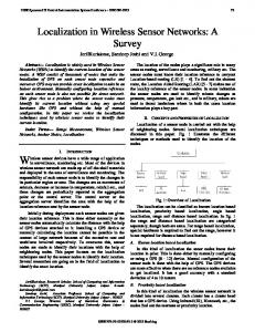
ments are represented using the adjacency matrix and the distance matrix. The goal is to obtain the estimation of the locations (s1 , s2 , · · · , sn−m ) ∈ ℜd of the remaining set of nodes V − H. Figure 9.1 illustrates an example of the above model. Five sensor nodes, whose locations are denoted as s1 , s2 , s3 , s4 , s5 , need to be localized with the help of four reference nodes with known locations r1 , r2 , r3 , r4 . The adjacency matrix and the distance matrix can be obtained given the proximity information collected at the sensor nodes and the anchors. Note that different sensors would have different number of reference nodes in their proximity. The accuracy of location estimates for the unlocalized sensors increases as a function of the number of reference nodes in the neighborhood.

r1

s3 r2

s5 s1

s4 r4

r3 s2

Fig. 9.1 An example of localization

9.2.1 Anchor-based Approaches Given densely deployed anchors in the network, the location of sensor nodes can be estimated with the help of the known locations of the anchors. A simple solution to the proximity based localization is to determine the Centroid, as proposed in [6]. It computes a node’s location approximated by the centroid of the locations of anchors in its proximity. Consider the example shown in Figure 9.1. The estimated locations of nodes s1 , s2 , s3 , s4 , s5 can be obtained as follows using the centroid technique:

290


(xs1 , ys1 ) = (xr4 , yr4 ) (xs2 , ys2 ) = (xr3 , yr3 ) xr + xr2 yr1 + yr2 , ) (xs3 , ys3 ) = ( 1 2 2 xr + xr3 + xr4 yr2 + yr3 + yr4 (xs4 , ys4 ) = ( 2 , ) 3 3 xr + xr3 yr2 + yr3 (xs5 , ys5 ) = ( 2 , ) 2 2 The accuracy of the centroid method relies heavily on the density of anchors. Low anchor density results in the deterioration in performance. The problem of low anchor density can be tackled through simple modifications to the centroid method. The underlying idea is to incrementally increase the density of reference node by including freshly localized nodes into the localization process. The modified method also allows anchors residing several hops away to be involved in localizing the nodes. However, this approach leads to the propagation of localization errors along with the location information. Weighted centroid or confidence-based centroid were introduced to address the problem of restricting error propagation in modified centroid methods [7, 8]. Localized nodes are assigned different weights or confidence levels in order to counterbalance the accumulation of location error from the localized nodes which act as anchors.

Fig. 9.2 Overview of APIT

To avoid the accumulation of location error in propagating the location information of anchor nodes, geometric characteristic of the spatial relationship among sensor nodes has been adopted in the graph theoretic techniques. An example is presented in APIT [9], in which the location of a non-anchor node can be inferred from the region it could possibly reside in. As shown in Figure 9.2, each non-anchor node runs the Point in Triangle (PIT) tests to find the triangle regions it resides in.


291

Each triangle region is formed by obtaining locations of three non-collinear anchors. The location of the non-anchor node is estimated to be the center of gravity of the intersection of the triangles, where the non-anchor resides. For proximity-based localization of static nodes, it is hard for the non-anchor nodes to perform the PIT test. The authors in [9] presented an approximate PIT test, in which the node is only required to be able to determine if any one of its neighbors is farther/closer to all the three anchors forming its residing triangle. Therefore, the location error of APIT roots in the approximate PIT test. Its performance relies heavily on the density of the network, where it is suggested that the degree of connectivity should exceed six.

r1 r2 C1 B2

B6

r0

C2

C5 A1

B3

r3

r6

C6

B1

C3

B4

B5 C4

r5

r4

Fig. 9.3 Deployment of anchors

The performance of proximity-based localization schemes depends on the positions of the anchor nodes. Intentional deployment of anchor nodes was exploited in [10] to divide the plane into location regions defined by the overlapping regions of sensing ranges of the anchors as shown in Figure 9.3. Instead of broadcasting its own position, an anchor node broadcasts the location regions consisting of its sensing range. For instance, the anchor node r0 sends out beacons containing the type {A, B,C} and the centroid of the location regions {A1 , B1 , · · · , B6 ,C1 , · · · ,C6 }, which are indeed the overlapping regions of the anchor nodes {r0 , r1 , · · · , r6 }. Upon receiving beacons from multiple anchors, the non-anchor node extracts the overlapping region of the anchors and take the centroid of the overlapping region as the estimate on its own location. Compared to APIT and the modified Centroid, the Cell Overlapping approach neither accumulates error in propagating the locations of anchors nor requires the RSSI value to perform the PIT test. To overcome the problem of low density of anchors, Gradient [11] and DVhop [12] focus on localizing non-anchor nodes with the knowledge of radio range

292


and locations of the anchors multiple hops away. The idea of Gradient is to estimate the distance between a pair of anchor and non-anchor nodes by multiplying hop count of the non-anchor nodes with the radio range. After obtaining distances to at least three anchors, the node applies multilateration algorithm to find out its own location. In contrast, DV-hop computes the average hop distance as anchors exchange their locations and hop count between them. After obtaining pairwise distances from a non-anchor node to an anchor by multiplying the average hop distance and the hop count from that anchor, triangulation is performed to estimate locations of the non-anchor nodes.

9.2.2 Anchor-free Approaches Multidimensional Scaling (MDS-MAP) [13] tackles the localization problem without using anchors. It estimates locations with the proximity information and the radio range. The MDS approach includes three steps. The first step is to form the distance matrix with distances between all pairs of nodes in the network. In the absence of anchors, the distance is inferred from the multiplication of the hop count and radio range. Then, in the second step, the Singular Vector Decomposition (SVD) is performed to determine an initial relative map of the nodes on the plane. The last step performs the necessary flip, rotation and scaling according to the distances between anchors if there is any. Otherwise, the relative map would be the result of SVD. It was shown that the time complexities of the first two steps are both O(n3 ), where n is the number of nodes in the network. The MDS approach is also applicable when only a few anchor nodes are available.

9.3 Range-based Localization Geometric techniques manage to estimate the locations of the sensor nodes from the range measurement and geometric computations. The underlying idea is that Euclidean distance between two sensor nodes can be measured by their radio signals through RSSI, TOA, TDOA etc. The presence of anchor nodes also plays an important role in geometric techniques in terms of the complexity of the problem and the difference between the localization goals: absolute versus relative locations.

9.3.1 Range Measurements Since the nodes are equipped with radios to perform communications, the distance estimation by measuring the radio signal strength has attracted lot of attention [14]. A simplified model for RSSI based range measurement is given by the following


equation:

RSSI ∝ d −α ,

293

(9.1)

where d is the distance and α is a constant relevant to the environment. Given a RSSI value measured by the radio, the radio receiver is able to infer its distance from the sender. However, RSSI based range measurement is extremely susceptible to noises and known for unreliability. An improvement on RSSI range measurements is proposed in [15] to reduce the distance estimation error by calibrating the range errors with RSSI values between known locations. Efforts have been made to obtain the mapping between RSSI measurements and the associated distances capturing the impacts of multipath fading, variations in temperature and humidity, human mobility and change in space layout on RSSI measurements in indoor localization [16]. The approaches based on probabilistic model of RSSI range measurements are also introduced to address the uncertainties and irregularities of the radio patterns. For instance, a log-normal model was adopted in [17], which assumes that a particular RSSI value can be mapped to a log-normal distribution of the distance between the two nodes, as in Equation (9.2). RSSI −→ lg d ∼ N(µ , σ ),

(9.2)

where d is the distance between the nodes, and N(µ , σ ) is a normal distribution with mean µ and standard deviation σ . Another common method for range measurement is based on the time difference of arrivals (TDOA). It estimates the distance between the nodes from measurements on the time differences of arrivals of signals. The signal could be radio frequency (RF), acoustic or ultrasound [18–20]. An example of utilizing TDOA was introduced in [21]. As shown in Figure 9.4, the radio signal and ultrasound pulses are sent simultaneously. Given the time difference of the arrivals, the distance between the sender and the receiver can be obtained by multiplying the time difference and the speed of the ultrasound signal. Similarly, ranging techniques based on the time of arrival (TOA), which rely on capturing the signal’s time of flight, obtain the distance by multiplying the time of flight with the signal speed [22]. The major challenge facing TOA based ranging techniques is the difficulty of accurately measuring the time of flight, since the propagation speed could be extremely high compared to the distance to be measured.

9.3.2 Localization Problems Using Range Measurements Given accurate range measurements, the localization algorithms are expected to produce the exact locations instead of raw estimations obtained from the proximitybased localization. The Euclidean distances between nodes can be interpreted both geometrically and mathematically. And the distance could be from one reference node to a non-localized node, denoted by di, j , or between two non-localized nodes, denoted by d i, j .

294

Sajal K. Das and Jing Wang and R. K. Ghosh and Rupert Reiger Sender

Receiver

RF

Ultrasound

δ

Fig. 9.4 An example of TDOA

The locations of the nodes satisfy the following equations: ∥ si − s j ∥2 = d¯i, j ∥ ri − s j ∥2 = di, j

D D

D C

B E A

C

A

C

B

A (a)

(b)

B (c)

Fig. 9.5 Graph rigidity

Although computing the distances between each pair of locations is a trivial problem, the inverse problem, which tries to find locations of the nodes given the Euclidean distances between each pair of nodes is far from trivial. It can be formulated as a graph realization problem, aiming at mapping the nodes in the graph to points in the plane so that the Euclidean distances between nodes equals the respective edge weights. The fundamental problem in graph realization is the rigidity of the graph, For example, as shown in Figure 9.5(a) and 9.5(b), non-rigidity is exhibited. Given a set of nodes and the Euclidean distances between each pair of nodes, the locations of nodes may not be unique. An example of a rigid graph is provided in Figure 9.5(c), in which the nodes are uniquely localized given the distances. More discussions on graph rigidity and network localization can be found in [23].


295

The study in [24] proved that the localization with distance information in sparse networks is an NP-hard problem, while localization with distances of Ω (n2 ) pairs of nodes can be solved in polynomial time [25].

9.3.3 Anchor-based Approaches Multilateration can be applied to obtain exact coordinates of a non-anchor node, given at least three anchors in the non-anchor node’s proximity and the pairwise measurements between the anchor and non-anchor nodes. Assume that the coordinates of m anchors are available, and that the distances between nodes can be obtained through ranging techniques. Let di j denote the measurement of distance between the ith anchor and the jth non-anchor node. The multilateration problem concerning localization is then formulated as follows: √ di j = (xi − x j )2 + (yi − y j )2 (9.3) The estimation error E j of the jth node is given by: m

E j = ∑ (di j − dî j )2 ,

(9.4)

i=1

where dî j is the estimated distance obtained by substituting the coordinates of the jth node with the estimated coordinates in Equation (9.3). Gradient descent can be applied to obtain the coordinates of the jth node achieving the least squared error. A similar approach was presented in [26]. The low density of anchors poses a challenge to the multilateration approach. In order to apply multilateration, DV-distance [27] follows the similar approach as DV-hop [12]. The distances of each hop are summed up to approximate the distance between a non-anchor node and an anchor node that is multiple hops away. The approximated distance is then used in the localization process. Instead of approximation of the multihop distance, the Euclidean method was proposed to compute the true distance through geometric relationships and the single hop distances. A detailed discussion on a localization protocol that follows the similar idea of Euclidean can be found in [28]. An example of multihop localization is demonstrated in Figure 9.6. According to DV-distance, the distance between the non-anchor node A and the anchor node D can be approximated as dAB + dBC or dAD + dCD depending on a certain voting mechanism. In contrast, the Euclidean method manages to obtain the multihop distance dAC by exploiting the geometric property of the quadrilateral ABCD. Although Euclidean focuses on computing the true distance to the anchor, it faces the rigidity problem due to low density of nodes. Given the set of single hop distances, the position of node A is not unique. As shown in Figure 9.6, node A′ leads to the same range measurements as node A. Additional neighbors and the corresponding range

296


B dBC

dAB dBD

dAC

C

A dCD dA’C

dAD D

A’

Fig. 9.6 Multihop localization

measurements are needed to eliminate the false estimation. According to [29], “an average of 11-12 degree of nodes in the ranging neighborhood” is required to have 90% of the network to be localized with a localization error of 5%. An iterative algorithm adopting the similar idea can be found in [30]. A tradeoff between energy efficiency and location accuracy is unveiled in the multihop localization approaches facing low density of anchors. The cost of Euclidean is higher than DV-hop due to the collaboration among neighboring nodes in order to compute the true Euclidean distances. Whereas, DV-hop suffers from higher location error introduced by the approximation of multihop distances. Although the semi-definite programming (SDP) approach [31] can be modified to incorporate the range measurements in the localization process by replacing the approximated distances with the measured distances, it tends to produce large localization error when the anchors are placed in the perimeter of the area. A different SDP problem is formulated in [32]. It manages to improve the localization performance by relaxing the equality constraint to the inequality constraint. The original problem of localizing n nodes using m anchors is formulated as follows: X ∈ R2×n ,Y ∈ Rn×n

Find such that

(

(9.5)

(ei − e j ) j6n ) ( )( ) I2 X αk αk T = d 2jk , ∀ j 6 n, k 6 m −e j −e j XT Y T

Y (ei − e j ) = d 2ji , ∀i,

Y = X T X, where αk is the locations of the m anchors, ei is a vector with zeros except the ith entry, d ji is the distance between the ith and jth non-anchor nodes pair, d jk is the distance between the kth anchor node and the jth non-anchor node. The above localization problem can be transferred into a standard SDP feasibility problem by changing Y = X T X to Y > X T X, which is equivalent to


( Z=

I X XT Y

297

) >0

The corresponding SDP problem is defined as follows: Find

Z ∈ R(n+2)×(n+2)

such that

(1; 0; 0)T Z(1; 0; 0) (0; 1; 0)T Z(0; 1; 0)

(9.6) =1 =1

(1; 1; 0)T Z(1; 1; 0) = 2 (0; ei − e j )T Z(0; ei − e j ) = d 2ji , ∀i, j 6 n (αk ; −e j )T Z(αk ; −e j ) = d 2jk , ∀ j 6 n, k 6 m Z>0 In order to guarantee that the solution of the SDP in Equation (9.6) is indeed the solution to the original problem in Equation (9.5), accurate distance measurements of 2n + n(n + 1)/2 pairs of nodes are required. Given noisy range measurements, the SDP problem can be formulated using the inequality constraints instead of the equality constraints on distances between nodes. The computation complexity of SDP is O(n3 ). Since it is expensive to apply the SDP method in localizing the whole network in a centralized process, a distributed SDP method was presented to address the scalability. While plain MDS has been proposed in localization with connectivity information, modified MDS methods were proposed to localize neighboring nodes with range measurements. An iterative MDS approach was presented in [33] to deal with the absence of some pairwise distances. It differs from the classic MDS approach by introducing weights wi j in the objective function as in Equation (9.7).

σ (X) = ∑ wi j (δi j − di j (X))2 ,

(9.7)

i< j

where σ (X) is the localization error with respect to the location vector X, δi j is the range measurements, di j is the distance computed from the location vector X, and wi j is the weight for each pair. For the absent pairwise range measurements, the corresponding weights are equal to zero, and the rest of the weights are ones. The location vector X is initialized using random values X (0) . The localization result X (k) obtained from the kth round is fed to the (k + 1)th round as the initial estimation on the location vector for the MDS process. The iteration stops when certain accuracy level is reached.

298


9.3.4 Anchor-free Approaches Considering the fact that using multilateration, non-anchor nodes could get localized relative to one another with a certain number of range measurements, DVcoordinates [27] promoted the idea of a two-stage localization scheme. During the first stage, neighboring nodes establish a local coordinate system according to the range measurements. Through registration with neighbors, the nodes transform their local coordinates into a global coordinate system in the second stage. Due to the insufficient overlapping or false overlapping between neighboring nodes, the performance of DV-coordinates suffers from error propagation in the second stage. The idea of DV-coordinates was explored further in [34]. It led to Robust Quad which become the building blocks of the local coordinate system in order to avoid flip ambiguity. First, the clusters consisting of overlapping Robust Quads are formed to establish the local coordinate system. As shown in Figure 9.5(c), the rigidity of the Robust Quad guarantees that two Robust Quad, ABCD and ABCE, sharing three vertices form a rigid subgraph with five vertices. The rigidity of the clusters is maintained by induction. Then, to mitigate the impact of noisy range measurements, a threshold on the minimum angle of the Robust Quad was introduced. With all these efforts, Robust Quad is able to significantly reduce the location error in comparison with other similar approaches.

B (x ,y ) B B (xC,yC) C A (0,0) Fig. 9.7 Triangulation example

Triangulation, as proposed in [1], is able to set up a local coordinate system with three nodes and their pairwise distances. A triangulation example is depicted in Figure 9.7. Node A tries to localize its neighbors B and C. A defines its own position as the origin of the local coordinate system and C to be along its horizontal axis. The locations of A’s neighbors are as follows:


299

xC = 0 yC = dAC xB = dAB cos ∠BAC yB = dAB sin ∠BAC 2 − d2 d 2 + dAC BC ∠BAC = arccos AB 2dAB dAC Applying similar derivations, any node can transform its locations to the coordinate system of its neighbor with the knowledge of the locations in the two coordinate systems and the pairwise distances. Therefore, the rest of the network can adjust the locations to one particular local coordinate system. The propagation of one particular coordinate system involves high cost of collaboration among nodes, which is not favorable to the energy deficient wireless sensor nodes.

9.4 Techniques with Additional Hardware Angle-based localization reduces the difficulty of the localization problem with knowledge on proximity or distances. However, the cost of applying angle measurement is remarkably high because of the antenna array or multiple receivers mounted on the nodes.

9.4.1 Angle Measurement With the help of antenna array, it is possible for the nodes to measure the signal’s angle of arrival (AOA) [35]. More recently, the angles between different edges of the connectivity graph can be obtained through multiple ultrasound receivers [36]. The AOA technique is adopted to assist both proximity-based and range-based localization as it is capable of improving the localization performance. The idea of angle measurement is demonstrated in Figure 9.8, in which every node is able to measure the angle to its neighbor node and its own axis. For node A that is to be localized, it is aware of the two angles ∠ab and ∠ac. The angle information can provide additional support to the localization or even localize the nodes solely based on the angle information [26].

300


North ∠ab

A ∠ac

∠bc ∠ba B

∠ca

C ∠cb

Fig. 9.8 Angle measurement

9.4.2 Localization with Angle Measurement The difficulty of localization solely on angle information has been studied in [37]. Fortunately, the angle information can be combined with the proximity-based localization. With angle information on all pairs of edges in the network, it is possible to transform the proximity based localization problem from NP-hard to P class (polynomial-time solvable) irrespective of the number of anchor nodes available in the network. A more realistic scenario with angle information and knowledge on distances in a sparse network is further shown to be a problem in P, while it has been proved to be NP-hard to localize nodes in a sparse network solely with knowledge of the distances. Therefore, the AOA technique remains an attractive option for localization applications in spite of its cost and difficulty of deployment.

S

A

O S Fig. 9.9 Localization with two anchors

B


301 B

S

O

C

A

Fig. 9.10 Localization with three anchors

When nodes are enabled with AOA capability, localization using AOA can be reduced to multilateration by simple transformations. As presented in [26], given a number of anchors and the angle observations, non-anchor nodes obtain their locations through multilateration process. Examples of localization method using AOA are shown in Figure 9.9 and Figure 9.10. The anchors A and B are one-hop neighbors of non-anchor node S in Figure 9.9. The location of S is confined to the dashed sector, the node S observes the AOA to A and B in terms of the angles ∠ASB or ∠BSA. Alternatively, as shown in Figure 9.10, a triplet of anchors can localize onehop non-anchor node using the AOA measurement. The location of S is along the circumscribed circle for the anchors A, B and C. The idea is to build a multilateration equation with the location of the non-anchor node, the center and the radius of the circle, which can be derived from the angle observed by the non-anchor node and the locations of the two or three anchors in the proximity of the non-anchor node. After obtaining a number of multilateration equations, (xS − xOi )2 + (yS − yOi )2 = ri2

(9.8)

the location of the non-anchor node can be computed with similar techniques for localization based on range measurements. Although additional hardware is required for localization based on angle information, it is shown in [38] that the angle information can significantly reduce the difficulty of the localization problem based on solely range measurements. Besides, as shown in [29], the angle information can assist in localization by reducing the number of anchors and the network density in order to achieve satisfactory localization performance.

9.5 Techniques based on Iterative Process Local maps can be formed by running the iterative MDS over local range measurements. The alignment of the local maps is performed along the route from one anchor to another. In order to get absolute locations, at least three anchors are required

302


to be present in the neighboring local maps. For further discussions on stitching the local maps, the readers may refer to [39]. Forming clusters of nodes within the network has been regarded as an effective technique to improve performance of WSNs, especially for solving the scalability problem. Cluster-based local coordinate system has been proposed in [40] to set up a local coordinate system for a small subset of the network. The master nodes (cluster heads) are responsible for transforming the local coordinate systems into one global system. A counterpart of the cluster-based localization using only proximity information was presented in [41]. Another iterative technique is shown in dwMDS [42]. It not only formulates the MDS problem with a novel optimization objective (the weighted cost function over multiple range measurements of pairwise distances) but also adopts an iterative algorithm starting from an initial estimation on the locations. Thus, the computational complexity is reduced from O(n3 ) in simple MDS to O(nL), where n is the total number of nodes in the network and L is the number of iterations to satisfy a pre-defined accuracy level. dwMDS can also localize networks with no anchors by providing relative locations. Since the error can be propagated and accumulated with the iterations, the error management scheme deserves further attentions in order to improve the localization performance of iterative methods. The potential error control techniques include selecting localized neighbors with certain level of accuracy in the iterative updates [43].

9.6 Mobility-assisted Localization Mobility of sensor nodes can be exploited in the localization process. For instance, an efficient sensor network design proposed in [44] took advantage of coverage overlaps over space and time because of the mobility of sensor nodes. Mobility-assisted localization relieves WSNs from the significant cost of deploying GPS receivers and the pressure of provisioning energy for interacting with each other during the localization process. Anchor nodes equipped with GPS are capable of localizing themselves while moving. With the use of mobile anchor nodes, localization algorithms show significant savings on the installation cost and energy consumption, and also improves accuracy. In [45], an example scheme is proposed to localize static sensor nodes with one mobile beacon. As shown in Figure 9.11, the mobile beacon periodically broadcasts beacon packets containing its coordinates while traversing the area where static sensor nodes are deployed. Upon receiving the beacon packets, a sensor node is able to infer its relative location to the beacon according to the radio signal strength (RSS) of the beacon packet through Bayesian inference. The two key elements that are discussed by the authors [45] in their approach are calibration and beacon trajectory. 1. Calibration: In order to estimate the node’s relative location to the moving beacon using the received RSS, it is necessary to calibrate the system, thus obtain-


303

Fig. 9.11 Localization using a mobile beacon

ing the propagation characteristic of the beacon packet in the air. The probability distribution function of the distance with respect to the received RSS is established given the calibration data. 2. Beacon trajectory: It determines the coverage of localization, the number of beacon packets broadcast and the localization accuracy. It is argued that the closer a beacon moves to the sensor node, the better is the localization accuracy. As a beacon trajectory can be regarded as a connected line of placements of static anchor nodes, it is quite obvious that non-collinearity and fold-freeness are also important to the beacon trajectory.

Fig. 9.12 Mobile beacon and Bounding Box

The computational complexity of the above localization algorithm is O(n2 ) and the storage requirement is also O(n2 ). As a result, it is possible to implement the lo-

304


calization algorithms on sensor nodes. Alternatively, the sensor nodes can report the RSS to a base station to avoid expensive computation with increased communication cost. A similar method has been described in [46] as a special case. The idea is that each time a sensor node receives a beacon, it generates a quadratic constraint on its own location according to the radio range. Upon receiving all the beacon packets, the sensor node’s location can be restricted in an intersected area of several bounding boxes as shown in Figure 9.12.

Fig. 9.13 Perpendicular Bisector of a Chord

Unlike the above GPS-based localization using mobile beacon, it was proposed in [47] to localize the sensor node using radio range of sensor node instead of that of mobile beacon. The method is based on a geometry conjecture, named Perpendicular Bisector of a Chord, which states that that a perpendicular bisector of a chord passes through the center of the circle (see Figure 9.13 for an illustration). Given the conjecture on the Perpendicular Bisector of a Chord, it is possible to calculate a sensor node’s location from its view of mobile beacon’s movement. By maintaining a visitor’s list, a sensor node is able to determine which beacon packets are sent when the mobile beacon entering and leaving the sensor node’s radio range. As shown in Figure 9.14, the sensor node selects beacon packets to construct chords of its radio range and locate itself as the center of the circle. Their approach showed that range-free localization could also produce fine-grained location information with the help of mobile beacon’s location broadcasts. The key factors affecting the localization performance are the following: 1. Beacon Scheduling: Beacon packets are scheduled by adding a random jitter time to the period of beacon packet in order to avoid collisions among broadcasts from different beacons since the approach is not restricted to one mobile beacon. 2. Chord Selection: As the probability of localization failures increases for short chords, a threshold of the length of the chord is applied to the selection of chords. 3. Radio Range: Given a larger radio range, the localization error can be slightly reduced due to the larger threshold on the length of the chords.


305

Fig. 9.14 Localization using intersect of perpendicular bisector of two chords

4. Beacon Speed: Increased speed of mobile beacon movements can reduce the execution time of the localization because more beacon packets are sent during the same time period. However, it may also increase the localization error due to higher probability of selecting shorter chords.

9.7 Statistical Techniques For indoor localization scenarios, the RSSI measurements suffer from severe multipath effects. Statistical approaches are regarded as promising candidates in dealing with noises and uncertainties of the measurements. The attempts to localize objects in the indoor environment with statistical techniques can be divided into two classes. One relies on mappings between the RSSI measurements and the locations, while the other manages to capture the statistical relationship between RSSI measurements and the distances. Both can work with off-line recording and on-line measurements in localizing the objects with RSSI measurement capability. An example of mapping the RSSI profile of the space is RADAR [48], which involves two stages. As shown in Figure 9.15, the RSSI values from multiple base stations (acting as anchors) are recorded at various locations during the first stage. Following this, a three-step localization process is performed in the second stage. In the first step, the object’s RSSI measurements from the base station are preprocessed for future matching. The sample mean of the multiple measurements to the base station can be adopted to represent the object’s location in the signal space. In second step, an RSSI map of the space is generated from either the empirical data or the propagation model akin to the empirical data. In the final step, the sample mean of the RSSI values from the base station is matched with its nearest neighbor in the signal space.

306


Fig. 9.15 Two-stage RADAR

The major difficulty of implementing RADAR comes from the off-line recording of the RSSI from the base stations. The off-line process of recording RSSI is not cost efficient, because location information needs to be collected together with the RSSI value at pre-determined spots in the indoor space. A kernel based learning method, aiming at relieving the system from cumbersome off-line preparation, was proposed in [49]. The idea is to formulate the localization problem as a pattern recognition problem with its kernel matrix established on the signal strength matrix, whose entries are the pairwise radio signal strength values collected at sensor nodes. The method requires training data in the learning process. However, the training data can be obtained through automated signal collecting phase involving the anchors and RSSI measurements between pairs of anchors. The pattern recognition algorithm focuses on determining the regions that each node resides in. The centroid of the intersection of the regions, a node belongs to, is thus regarded as the node’s location. Although the localization process of the kernel-based learning method can be executed locally, its training process is inevitably centralized and computation extensive. A fully distributed localization method without explicit statistical model for range measurement was presented in [50]. The location of nodes are represented by the exact locations and the corresponding uncertainties. Each node computes its belief of the location, which is a normalized estimate of the posterior likelihood of the location. The node communicates with neighbors on each other’s belief and updates its location and the associate belief based on the received information from neighbors. The process iterates until certain convergence criteria are met. The fully


307

distributed algorithm relies on local information and message exchanges, which invokes less communication and computation costs as compared with centralized algorithms. LaSLAT [51] is a framework, based on Bayesian filters to accomplish the task of localizing mobile nodes, in which the location estimates are iteratively updated given batches of new measurements. Extensive empirical studies have shown that LaSLAT can tolerate noisy range measurements and achieve satisfactory location accuracy. The Kalman filter and particle filter are essentially variants of Beyesian filters, which estimate the state of a dynamic system statistically through noisy measurements. Kalman filters approximate the belief of the state by its first and second order moments and achieve the optimality when the initial uncertainty follows Gaussian distribution. In contrast, particle filters realize the Bayesian filter using sets of samples with different importance factors. More discussion on the Bayesian filter and localization can be found in [52]. Statistical approaches are capable of tackling the difficulty of localization introduced by the mobility of nodes. Monte Carlo Localization (MCL) method was adopted in [53] to solve the localization problem in mobile sensor networks. It follows an approach similar to the Bayesian filter. Unscented Kalman Filter, inspired by MCL, which produces location estimates from a subset of samples, was used to localize mobile nodes through passive listening [54]. An alternation to the map-assisted localization is the probabilistic model based location, in which probabilistic models for range measurements and location estimates are introduced instead of deterministic relationships between range measurements and location estimates. A method, proposed in [55], is based on the probabilistic model of RSSI that is obtained from calibration data corresponding to an outdoor environment without obstructions. The model is given by the following: p → lgD ∼ N(µD (p), σD (p)) µD (p) = lgde+ σD2 ln10 σP σD (p) = σD = 10η

(9.9) (9.10) (9.11)

where the distance associated with a particular RSSI value follows a log normal distribution, σP is the variance of the RSSI value, η is the coefficient determined by calibration, and de is the average of the distance regarding a particular RSSI value. The log normal model has been verified by the experiment data. Then the conditional probability density function of the distance can be approximated using Equation (9.12) given RSS measurement with Ps and σP (s).

ξ (s|p) fD (s|p) = ∫ ∞ 0 ξ (s|p)ds where

(9.12)

308

Sajal K. Das and Jing Wang and R. K. Ghosh and Rupert Reiger − 1 ξ (s|p) = √ e 2πσ p (s)

(p−P(s))2 2 (s) 2σP

.

Initially, the non-anchor node has the estimation of their location to be evenly distributed in the deployment area. After receiving packets from neighboring nodes, either anchor or non-anchor nodes update their estimations on the probability density function (pdf) of the distance. Therefore, the location estimation for the nonanchor nodes can be updated accordingly. Additionally, a Bayesian model for the noisy distance measurements was reported in [56]. The model is demonstrated in Figure 9.16. In the above Bayesian graphical model, conditional density for each vertex are: X: uniform(0,L), x-ordinate of node, where L is the width of the region. Y : uniform(0,B), y-ordinate of node, where B is the length of the region. Si : N(bi0 + bi1 logDti , τi ), i = 1, 2, 3, 4, RSS, where Dti is the distance to the ith access point (anchor node). bi0 : N(0,0.001), i = 1, 2, 3, 4. bi1 : N(0,0.001), i = 1, 2, 3, 4. where uniform represents uniform distribution and N(µ , τ ) stands for Gaussian distribution with µ mean and τ standard deviation.

Fig. 9.16 Bayesian graphical models (from left to right): Bayesian graphical model, Hierarchical Bayesian graphical model, Hierarchical Bayesian graphical model with a corridor effect [56]

A hierarchical Bayesian graphical model is brought up in order to incorporate the prior knowledge of linear regression models in accordance with the access points that the coefficients of the models are similar to each other. The conditional density for the vertexes are:


309

X: uniform(0,L), Y : uniform(0,B). Si : N(bi0 + bi1 logDti , τi ), i=1, · · · , d. bi0 : N(b0 , τb0 ), i = 1, · · · , d, b0 : N(0, 0.001), and τb0 : Gamma(0.001,0.001). bi1 : N(b1 , τb1 ), i = 1, · · · , d, b1 : N(0,0.001), and τb1 : Gamma(0.001,0.001). where Gamma represents the Gamma distribution. Both of the models are trained with measurement data. A surprising observation on the training result is that the location information of the RSS data does not affect the localization performance obtained from the hierarchical Bayesian graphical model given same amount of sample size. This observation indicates a promising benefit of using hierarchical Bayesian graphical model. When the RSS data are collected, it is not necessary to collect the location associated with the RSS data. It will save a lot of cost on profiling RSS inside a building. Besides the modeling efforts using particular distributions, an empirical study on the statistical characteristics based on probability density functions can be found in [57].

9.8 Summary on Localization Techniques The focus of our discussion in this section is on the evaluation of localization schemes. The ability to fix the position of a sensor node in terms of absolute location would determine the effectiveness of a particular localization scheme. But, in the absence of GPS or specialized measurement hardware, certain amount of error is bound to creep in. So there is need for qualitative evaluation of the localization schemes.

9.8.1 Localization Accuracy An extensive body of literature exists on the error analysis that examines the accuracy of estimated locations obtained from various localization schemes. According to the localization process, the sources of localization error may include: physical sources, localization algorithms, refinement process [58, 59]. The errors due to physical sources are represented by wide range of noises and quantization losses. Ranging techniques vary from ultrasonic to radio, and to laser, etc. A summary on the range accuracy was presented in [60]. Table 1 presents a comparison of ranging errors among different range based techniques. The most attractive among these are the ones with low cost and ready-to-use features like time of arrival (TOA) of ultrasonic signal and Radio Signal Strength (RSS) or Radio Signal Strength Indication (RSSI). The only concern about these techniques is that they produce highly noisy measurements and are over sensitive to environmental effects. Localization algorithms encounter two types of error sources. One is system error, which comes from the localization algorithms themselves that work with under-

310


Table 9.1 Expected Accuracy of Different Measurement Technologies [60]

Technology Ultrasound Ultra Wide Band RF Time of Flight Laser Time of Flight

System AHLoS PAL UWB Bluesoft Laser range finder

Accuracy 2cm 1.5m 0.5m 1cm

Range 3m N/A 100m 75m

lying assumption of accurate range measurement or range-free features. The other source of error is related to connectivity and the fraction of nodes serving as anchors. The last two parameters have significant impacts on the performance of localization algorithms. The effect of system error becomes manageable, when both distance and angle with orientation are available. But the size and the cost of the hardware capable of measuring distance and angle prevent such system from implementation, especially for dense WSNs. It is of particular interest to study the impact of range errors on the performance of localization algorithms, because range errors are inherent to WSNs employing simple and low-cost range measurement hardware. According to the empirical study on the impact of range errors on multihop localizations [61], high density and Gaussian noises are the two pre-requisites for the noisy disk model to work. The study also suggests statistical approaches fixing the problem resulted from range errors. Cramer-Rao Lower Bound (CRLB) is commonly adopted in the error analysis of the localization schemes. It is a lower bound on the variance of the estimator that estimates the locations. Given the knowledge on the distribution of measurements, it is shown in [62–64] that the bound on the localization error can be obtained through calculating the CRLB. Therefore, the localization schemes are able to evaluate their performances by comparing the localization accuracy with the corresponding CRLB.

9.8.2 Computation and Communication Costs As energy efficiency is critical to WSNs, it is necessary to consider the computation and communication costs of the localization process in the evaluation of localization schemes. Centralized algorithms like the SDP or MDS-MAP demand range measurements from all the nodes. This is expensive in terms of forwarding the measurements to the processing point and solving the high dimension matrix. Distributed algorithms, on the other hand, require collaborations among neighboring nodes to some extent. In particular, the multihop localization faces the tradeoff between the communication cost on propagating the anchor-locations and the degree of accuracy. For the refinement on location estimations, the number of iterations are apparently in the center of the tradeoff between the energy consumption for refinement of localization results and the degree of accuracy achievable through refining.


311

9.8.3 Network and Anchors Density It is worth noticing that localization algorithms always require a certain level of connectivity. So, localization schemes are based on connectivity, range measurements, angle information or any combinations thereof. The discussions on the localization algorithms suggest that dense networks lead to better localization performance. However, a dense network does not necessarily guarantee high accuracy in location estimations. The density of the network is usually represented by the number of nodes within an area or the radio range of nodes. The anchor-based localization schemes, aiming at providing absolute locations, require a high density of anchors to ensure low level of localization errors [65].

9.8.4 Summary of Performances In the previous sections, existing localization schemes were discussed under various scenarios. The difficulty in comparing them is exacerbated by the fact that different testbeds for the evaluation purpose are built separately. In the following, let us summarize the performance of these schemes with respect to accuracy, communication/computation costs and node density. Table 2 presents the simulation results of various localization schemes, where the accuracy was examined through the tradeoffs between accuracy and measurement performance, percentage of anchors, deployment of anchors, density of nonanchors, etc. Besides randomly generated networks, a typical deployment of nodes is the grid of non-anchor nodes within a particular area. The localization accuracy of a solution is usually quantified using the average Euclidean distance between the estimated locations and the true locations normalized to the radio range or other system parameters. For mobility-assisted localization, the effect of node density is not as important as in static localization scenarios. In addition, communication/computation cost may not be of same importance to the off-line simulations as to the real implementations. The table only shows typical values for the items when various tradeoffs for one solution were reported in the literature. For the sake of conciseness, radio range and node degree are denoted by R and dg respectively in the table, while D represents the average inter-distance of anchors and n is the number of nodes to be localized in the network. Some of the empirical results of localization schemes are listed in Table 3. The number of anchors is usually low due to the cost and the difficulty of deployment. These results echo the report on the high accuracy achieved by ultrasound ranging techniques. The analysis on the communication/computation costs was not extensively presented in the empirical studies due to the difficulty in measuring the cost in real implementations.

312


Table 9.2 Summary of Simulation Results for Various Localization Schemes Methods Accuracy Computation/Communication Cost Node Density APIT [9] 40%R 10% Message Overhead of DV-hop 16 one-hop anchors Gradient [11] 10%R N/A 4 anchors at the corners DV-hop [12] 30%R for isotropic; 90%R for anisotropic 7000 messages exchanged dg=7.6 with 30% to be anchors DV-distance [12] 15%R for isotropic; 80%R for anisotropic 7200 messages exchanged dg=7.6 with 30% to be anchors Euclidean [12] 10%R for isotropic; 15%R for anisotropic 8000 messages exchanged dg=7.6 with 30% to be anchors 3 MDS-MAP [13] 50%R computation complexity of O(n ) dg>12.2 with 3 anchors at random positions Ecolocation [66] 30%D N/A 15 anchors randomly placed DV-coordinate [27] 1m for isotropic; 1.25m for anisotropic N/A dgaverage =9 DV-bearing [26] 1 hop distance N/A dgaverage =10.5 DV-radial [26] 0.8 hop distance N/A dgaverage =10.5 Bisector [47] 5%R 1597 packets 319 randomly deployed nodes Kernel-based Learning [49] 0.47 worst case computational time O(n3 ) 25 anchors, 400 non-anchors EKF [67] 20%R N/A randomly deployed nodes, 1 mobile robot MCL [53] 20%R 50 samples dg=10, anchor density is 4 RSS Model [17] 5%R O(n2 log2 n) node density is 0.5/meter2

9.9 Open Issues There has been extensive research on sensor localization, however, there are some important open issues specially relevant to sensor nodes in a WSN which either remain unresolved or not explored extensively. Some of these issues are listed below. 1. Energy Consumption Although energy consumption has been addressed in the study on localization with WSNs, the energy efficiency goal of the localization schemes remains challenging. The problem of minimizing energy consumption of the localization process deserves further attention. As the energy consumption of the localization application involves measurements, communication with neighbors and estimation of locations, the task of quantifying the energy consumption demands system-wide efforts to incorporating energy efficient design at all communication layers and all aspects of the localization algorithm. 2. 3-Dimension Localization The typical scenario for localization with WSNs is to find out locations of the nodes in a 2-D plane. However, nodes are usually deployed in a 3-D space, which leads to differences on both ranging results and localization algorithms. Analysis on localization schemes focusing on the 3-D space is of particular interests to real applications of WSNs, especially when the difference between 2-D space and 3-D space is significant. For instance, irregularity of the radio transmission has been investigated in 2-D space, while its counterpart in 3-D space remains to be unknown [68, 69]. 3. Security and Privacy Security and privacy have always been the fundamental issues in large scale deployment of WSNs. Since locations of nodes are of importance to the applications’ tasks, the security of the location needs to be guaranteed. Although some researches on security of localization schemes are presented [70, 71], the types of attacks and the related countermeasures are restricted to a few typi-


313

Table 9.3 Table 3 Summary of Empirical Results Methods Centroid [6] Classic MDS [42] MLE [42] dwMDS [42] Ecolocation (outdoor) [66] Ecolocation (indoor) [66] Robust Quad [34] Multilateration [21, 45] Mobile Beacon [45] RADAR [48] Kernel-based Learning [49] LaSLAT [51]

Accuracy Computation/Communication Cost Node Density 1.83m N/A 4 anchors at corners, grid of non-anchors 4.3m for RSS; 1.96 for TOA O(n2 T ) operations 4 anchors at corners 2.18m for RSS; 1.23 for TOA N/A 4 anchors at corners 2.48m for RSS; 1.12 for TOA O(nL) 4 anchors at corners 20%D N/A 11 nodes with full connectivity 35%D N/A 12 anchors, 5 non-anchors 5.18cm for ultrasound ranging N/A dg=12, total 40 nodes 10.67m N/A range data from 1 mobile beacon 1.4m N/A 12 non-anchors, 1 mobile beacon 3m N/A dg=3, 3 anchors 3.5m N/A grid deployment of 25 anchors and 81 nodes 1.9cm for ultrasound ranging N/A dg=10, total 27 nodes

cal cases. Similarly, researches on privacy of nodes’ locations mostly focus on preventing the locations of data sources or base stations from being exposed to adversaries [72, 73]. The existing sensor localization schemes have not been fully examined from the perspective of privacy protection.

9.10 Conclusions In this chapter, we discussed sensor localization from its algorithmic aspects. Graph theoretic techniques solve the localization problem through modeling the proximity information collected by the sensor nodes into edges of the graph and the nodes themselves vertices. In order to reduce the estimation error on nodes’ locations, geometric based techniques were proposed to incorporate the distance measurements between pairwise nodes in the localization process. Furthermore, techniques with additional hardware explores the geometric characteristic of the network by introducing the angle measurements. Besides, iterative techniques focus on refining the initial estimation of the locations until the goal of high estimation accuracy is achieved. In contrast to localization of static sensor nodes, mobile-assisted localization techniques exploit the presence of mobile nodes that have abundant resources. The mobile nodes are able to tackle the problem of low density of anchors in the network by moving around static sensor nodes acting as the anchor. However, mobility poses additional difficulty to the sensor localization problem when all the sensor nodes are mobile. Statistical techniques are able to accomplish the localization task for mobile nodes with the help of statistical models for range measurements and the learning mechanism. The comparison among the existing algorithms for sensor localization shows that energy efficiency of the localization process remains to be a critical issue for wireless sensor networks, while security and privacy in sensor localization among other open issues expect further investigations. Acknowledgements This work is partially supported by an EADS grant and NSF grants CNS0916221 and CNS-0721951.

314


References 1. S. Capkun, M. Hamdi, and J.-P. Hubaux, “GPS-free positioning in mobile ad-hoc networks,” Proceedings of the 34th Annual Hawaii International Conference on System Sciences, 2001. 2. G. Mao and B. Fidan, “Localization algorithms and strategies for wireless sensor networks,” Information Science Reference - Imprint of: IGI Publishing, 2009. 3. A. Savvides, M. Srivastava, L. Girod, and D. Estrin, “Localization in sensor networks,” In Wireless sensor networks, C. S. Raghavendra, K. M. Sivalingam, and T. Znati, Eds. Kluwer Academic Publishers, Norwell, MA, pp. 327–349, 2004. 4. J. Bachrach and C. Taylor, “Localization in sensor networks”. In Handbook of Sensor Networks: Algorithms and Architectures, Ivan Stojmenovic Eds. John Wiley & Sons, ch. 9, pp. 277–310, 2005. 5. G. Mao, B. Fidan, and B. D. O. Anderson, “Wireless sensor network localization techniques,” Comput. Netw., vol. 51, no. 10, pp. 2529–2553, 2007. 6. N. Bulusu, J. Heidemann, and D. Estrin, “GPS-less low-cost outdoor localization for very small devices,” IEEE Personal Commun. Mag. [see also IEEE Wireless Commun. Mag.], vol. 7, no. 5, pp. 28–34, 2000. 7. P. Agrawal, R. K. Ghosh, and S. K. Das, “Localization of wireless sensor nodes using proximity information,” ICCCN 2007: the 16th International Conference on Computer Communications and Networks, 2007. 8. R. Salomon, “Precise localization in coarse-grained localization algorithms through local learning,” IEEE SECON 2005: Second Annual IEEE Communications Society Conference on Sensor and Ad Hoc Communications and Networks, pp. 533–540, 2005. 9. T. He, C. Huang, B. M. Blum, J. A. Stankovic, and T. F. Abdelzaher, “Range-free localization and its impact on large scale sensor networks,” Trans. on Embedded Computing Sys., vol. 4, no. 4, pp. 877–906, 2005. 10. H.-C. Chu and R.-H. Jan, “A GPS-less, outdoor, self-positioning method for wireless sensor networks,” Ad Hoc Networks, vol. 5, no. 5, pp. 547–557, 2007. 11. R. Nagpal, H. Shrobe, and J. Bachrach, “Organizing a global coordinate system from local information on an ad hoc sensor network,” IPSN 2003: Proceedings of the 3rd International Symposium on Information Processing in Sensor Networks, 2003. 12. D. Niculescu and B. Nath, “Ad hoc positioning system (APS),” IEEE GLOBECOM 2001, pp. 2926–2931, 2001. 13. Y. Shang, W. Ruml, Y. Zhang, and M. P. J. Fromherz, “Localization from mere connectivity,” MobiHoc 2003: Proceedings of the 4th ACM International Symposium on Mobile Ad Hoc Networking & Computing, pp. 201–212, 2003. 14. K. Whitehouse, C. Karlof, and D. Culler, “A practical evaluation of radio signal strength for ranging-based localization,” SIGMOBILE Mob. Comput. Commun. Rev., vol. 11, no. 1, pp. 41–52, 2007. 15. R. Reghelin and A. A. Fröhlich, “A decentralized location system for sensor networks using cooperative calibration and heuristics,” MSWiM 2006: Proceedings of the 9th ACM International Symposium on Modeling Analysis and Simulation of Wireless and Mobile Systems, pp. 139–146, 2006. 16. H. Lim, L.-C. Kung, J. C. Hou, and H. Luo, “Zero-configuration, robust indoor localization: Theory and experimentation,” INFOCOM 2006: 25th IEEE International Conference on Computer Communications, pp. 1–12, April 2006. 17. R. Peng and M. L. Sichitiu, “Probabilistic localization for outdoor wireless sensor networks,” SIGMOBILE Mob. Comput. Commun. Rev., vol. 11, no. 1, pp. 53–64, 2007. 18. X. Cheng, A. Thaeler, G. Xue, and D. Chen, “TPS: a time-based positioning scheme for outdoor wireless sensor networks,” INFOCOM 2004: 23rd AnnualJoint Conference of the IEEE Computer and Communications Societies, vol. 4, pp. 2685–2696, 2004. 19. J. Zhang, T. Yan, J. A. Stankovi, and S. H. Son, “Thunder: towards practical, zero cost acoustic localization for outdoor wireless sensor networks,” SIGMOBILE Mob. Comput. Commun. Rev., vol. 11, no. 1, pp. 15–28, 2007.


315

20. M. Broxton, J. Lifton, and J. A. Paradiso, “Localization on the pushpin computing sensor network using spectral graph drawing and mesh relaxation,” SIGMOBILE Mob. Comput. Commun. Rev., vol. 10, no. 1, pp. 1–12, 2006. 21. A. Savvides, C.-C. Han, and M. B. Strivastava, “Dynamic fine-grained localization in ad-hoc networks of sensors,” MobiCom 2001: the 7th Annual International Conference on Mobile Computing and Networking, pp. 166–179, 2001. 22. M. Youssef, A. Youssef, C. Rieger, U. Shankar, and A. Agrawala, “PinPoint: An asynchronous time-based location determination system,” MobiSys 2006: the 4th International Conference on Mobile Systems, Applications and Services, pp. 165–176, 2006. 23. T. Eren, O. Goldenberg, W. Whiteley, Y. Yang, A. Morse, B. Anderson, and P. Belhumeur, “Rigidity, computation, and randomization in network localization,” INFOCOM 2004: the 23rd AnnualJoint Conference of the IEEE Computer and Communications Societies, vol. 4, pp. 2673–2684, 2004. 24. J. Aspnes, D. Goldenberg, and Y. R. Yang, “On the computational complexity of sensor network localization,” the 1st International Workshop on Algorithmic Aspects of Wireless Sensor Networks, pp. 32–44, 2004. 25. A. M.-C. So and Y. Ye, “Theory of semidefinite programming for sensor network localization,” Math. Program., vol. 109, no. 2, pp. 367–384, 2007. 26. D. Niculescu and B. Nath, “Ad hoc positioning system (APS) using AOA,” INFOCOM 2003: the 22nd Annual Joint Conference of the IEEE Computer and Communications Societies, vol. 3, pp. 1734–1743, 2003. 27. Dragos Niculescu and Bari Nath, “Dv based positioning in ad hoc networks,” Telecommunication Systems, vol. 22, no. 1-4, pp. 267–280, 2003. 28. Y. Zhang and L. Cheng, “PLACE: protocol for location and coordinate estimation: a wireless sensor network approach,” Comput. Netw., vol. 46, no. 5, pp. 679–693, 2004. 29. K. Chintalapudi, A. Dhariwal, R. Govindan, and G. Sukhatme, “Ad-hoc localization using ranging and sectoring,” INFOCOM 2004: the 23rd AnnualJoint Conference of the IEEE Computer and Communications Societies, vol. 4, pp. 2662–2672, 2004. 30. A. Savvides, H. Park, and M. B. Srivastava, “The bits and flops of the n-hop multilateration primitive for node localization problems,” in WSNA 2002: the 1st ACM International Workshop on Wireless Sensor Networks and Applications, New York, NY, USA: ACM, pp. 112–121, 2002. 31. L. Doherty, K. Pister, and L. E. Ghaoui, “Convex position estimation in wireless sensor networks,” INFOCOM 2001: the 20th Annual Joint Conference of the IEEE Computer and Communications Societies, vol. 3, pp. 1655–1663, 2001. 32. P. Biswas, T.-C. Lian, T.-C. Wang, and Y. Ye, “Semidefinite programming based algorithms for sensor network localization,” ACM Trans. Sen. Netw., vol. 2, no. 2, pp. 188–220, 2006. 33. X. Ji and H. Zha, “Sensor positioning in wireless ad-hoc sensor networks using multidimensional scaling,” INFOCOM 2004: the 23rd AnnualJoint Conference of the IEEE Computer and Communications Societies, vol. 4, pp. 2652–2661, 2004. 34. D. Moore, J. Leonard, D. Rus, and S. Teller, “Robust distributed network localization with noisy range measurements,” SenSys 2004: the 2nd International Conference on Embedded Networked Sensor Systems, pp. 50–61, 2004. 35. P. Stoica and K. Sharman, “Maximum likelihood methods for direction-of-arrival estimation,” IEEE Trans. Acoust., Speech, Signal Process., vol. 38, no. 7, pp. 1132–1143, 1990. 36. N. B. Priyantha, A. Chakraborty, and H. Balakrishnan, “The cricket location-support system,” MobiCom 2000: the 6th Annual ACM International Conference on Mobile Computing and Networking, 2000. 37. J. Bruck, J. Gao, and A. A. Jiang, “Localization and routing in sensor networks by local angle information,” MobiHoc 2005: the 6th ACM International Symposium on Mobile Ad Hoc Networking and Computing, pp. 181–192, 2005. 38. M. Bˇadoiu, E. D. Demaine, M. T. Hajiaghayi, and P. Indyk, “Low-dimensional embedding with extra information,” SCG 2004: the 20th Annual Symposium on Computational Geometry, pp. 320–329, 2004.

316


39. O.-H. Kwon and H.-J. Song, “Localization through map stitching in wireless sensor networks,” IEEE Trans. Parallel Distrib. Syst., vol. 19, no. 1, pp. 93–105, 2008. 40. R. Iyengar and B. Sikdar, “Scalable and distributed GPS free positioning for sensor networks,” ICC 2003: IEEE International Conference on Communications, vol. 1, pp. 338–342, 2003. 41. H. Chan, M. Luk, and A. Perrig, “Using clustering information for sensor network localization,” DCOSS 2005: IEEE Conference on Distributed Computing in Sensor Systems, 2005. 42. J. A. Costa, N. Patwari, and A. O. H. Iii, “Distributed weighted-multidimensional scaling for node localization in sensor networks,” ACM Trans. Sen. Netw., vol. 2, pp. 39–64, 2006. 43. J. Liu, Y. Zhang, and F. Zhao, “Robust distributed node localization with error management,” MobiHoc 2006: the 7th ACM International Symposium on Mobile Ad Hoc Networking and Computing, pp. 250–261, 2006. 44. S. Nikoletseas and P. Spirakis, “Efficient sensor network design for continuous monitoring of moving objects,” Theor. Comput. Sci., vol. 402, no. 1, pp. 56–66, 2008. 45. M. L. Sichitiu and V.Ramadurai, “Localization of wireless sensor networks with a mobile beacon,” IEEE International Conference on Mobile Ad-hoc and Sensor Systems, pp. 174–183, 2004. 46. A. Galstyan, B. Krishnamachari, K. Lerman, and S. Pattem, “Distributed online localization in sensor networks using a moving target,” IPSN 2004: the 3rd International Symposium on Information Processing in Sensor Networks, pp. 61–70, 2004. 47. K.-F. Ssu, C.-H. Ou, and H. Jiau, “Localization with mobile anchor points in wireless sensor networks,” IEEE Trans. Veh. Technol., vol. 54, no. 3, pp. 1187 – 1197, 2005. 48. P. Bahl and V. N. Padmanabhan, “RADAR: An in-building RF-based user location and tracking system,” INFOCOM 2000: the 19th IEEE International Conference on Computer Communications, pp. 775–784, 2000. 49. X. Nguyen, M. I. Jordan, and B. Sinopoli, “A kernel-based learning approach to ad hoc sensor network localization,” ACM Trans. Sen. Netw., vol. 1, no. 1, pp. 134–152, 2005. 50. E. T. Ihler, J. W. Fisher, O. L. Moses, and A. S. Willsky, “Nonparametric belief propagation for self-localization of sensor networks,” IEEE J. Sel. Areas Commun., vol. 23, pp. 809–819, 2005. 51. C. Taylor, A. Rahimi, J. Bachrach, H. Shrobe, and A. Grue, “Simultaneous localization, calibration, and tracking in an ad hoc sensor network,” IPSN 2006: the 5th International Conference on Information Processing in Sensor Networks, pp. 27–33, 2006. 52. D. Fox, J. Hightower, L. Liao, D. Schulz, and G. Borriello, “Bayesian filtering for location estimation,” IEEE Pervasive Comput., vol. 02, no. 3, pp. 24–33, 2003. 53. L. Hu and D. Evans, “Localization for mobile sensor networks,” MobiCom 2004: the 10th Annual International Conference on Mobile Computing and Networking, pp. 45–57, 2004. 54. L. Zhang, Q. Cheng, Y. Wang, and S. Zeadally, “Landscape: a high performance distributed positioning scheme for outdoor sensor networks,” WiMob 2005: IEEE International Conference on Wireless and Mobile Computing, Networking and Communications, vol. 3, pp. 430– 437, 2005. 55. R. Peng and M. L. Sichitiu, “Probabilistic localization for outdoor wireless sensor networks,” SIGMOBILE Mob. Comput. Commun. Rev., vol. 11, no. 1, pp. 53–64, 2007. 56. D. Madigan, E. Einahrawy, R. P. Martin, W. H. Ju, P. Krishnan, and A. S. Krishnakumar, “Bayesian indoor positioning systems,” INFOCOM 2005: the 24th Annual Joint Conference of the IEEE Computer and Communications Societies, pp. 1217–1227 vol. 2, 2005. 57. A. Cerpa, J. L. Wong, L. Kuang, M. Potkonjak, and D. Estrin, “Statistical model of lossy links in wireless sensor networks,” IPSN 2005: the 4th International Symposium on Information Processing in Sensor Networks, 2005. 58. S. Slijepcevic, S. Megerian, and M. Potkonjak, “Location errors in wireless embedded sensor networks: sources, models, and effects on applications,” SIGMOBILE Mob. Comput. Commun. Rev., vol. 6, no. 3, pp. 67–78, 2002. 59. H. A. Oliveira, E. F. Nakamura, A. A. F. Loureiro, and A. Boukerche, “Error analysis of localization systems for sensor networks,” GIS 2005: the 13th Annual ACM International Workshop on Geographic Information Systems, pp. 71–78, 2005.


317

60. A. Savvides, W. Garber, R. Moses, and M. Srivastava, “An analysis of error inducing parameters in multihop sensor node localization,” IEEE Trans. Mobile Comput., vol. 4, no. 6, pp. 567–577, Nov.-Dec. 2005. 61. K. Whitehouse, C. Karlof, A. Woo, F. Jiang, and D. Culler, “The effects of ranging noise on multihop localization: an empirical study,” IPSN 2005: the 4th International Symposium on Information Processing in Sensor Networks, pp. 73–80, 2005. 62. N. Patwari, I. A.O. Hero, M. Perkins, N. Correal, and R. O’Dea, “Relative location estimation in wireless sensor networks,” IEEE Trans. Signal Process. , vol. 51, no. 8, pp. 2137–2148, 2003. 63. C. Chang and A. Sahai, “Estimation bounds for localization,” SECON 2004: the 1st IEEE Communications Society Conference on Sensor and Ad Hoc Communications and Networks, pp. 415–424, 2004. 64. S. Venkatesh and R. M. Buehrer, “Multiple-access insights from bounds on sensor localization,” Pervasive Mob. Comput., vol. 4, no. 1, pp. 33–61, 2008. 65. N. Bulusu, J. Heidemann, D. Estrin, and T. Tran, “Self-configuring localization systems: Design and experimental evaluation,” Trans. on Embedded Computing Sys., vol. 3, no. 1, pp. 24–60, 2004. 66. K. Yedavalli, B. Krishnamachari, S. Ravula, and B. Srinivasan, “Ecolocation: a sequence based technique for RF localization in wireless sensor networks,” IPSN 2005: the 4th International Symposium on Information Processing in Sensor Networks, pp. 285–292, 2005. 67. K. Sreenath, F. L. Lewis, and D. O. Popa, “Simultaneous adaptive localization of a wireless sensor network,” SIGMOBILE Mob. Comput. Commun. Rev., vol. 11, no. 2, pp. 14–28, 2007. 68. A. Y. Teymorian, W. Cheng, L. Ma, X. Cheng, X. Lu, and Z. Lu, “3d underwater sensor network localization,” IEEE Trans. Mobile Comput., vol. 8, pp. 1610–1621, 2009. 69. H. S. Abdelsalam and S. Olariu, “A 3d-localization and terrain modeling technique for wireless sensor networks,” in FOWANC 2009: the 2nd ACM International Workshop on Foundations of Wireless Ad Hoc and Sensor Networking and Computing. New York, NY, USA: ACM, pp. 37–46, 2009. 70. Z. Li, W. Trappe, Y. Zhang, and B. Nath, “Robust statistical methods for securing wireless localization in sensor networks,” IPSN 2005: the 4th International Symposium on Information Processing in Sensor Networks, pp. 91–98, 2005. ˇ 71. L. Lazos, R. Poovendran, and S. Capkun, “ROPE: robust position estimation in wireless sensor networks,” IPSN 2005: the 4th International Symposium on Information Processing in Sensor Networks, 2005. 72. M. Shao, Y. Yang, S. Zhu, and G. Cao, “Towards statistically strong source anonymity for sensor networks,” in INFOCOM 2008: the 27th IEEE International Conference on Computer Communications, pp. 51–55, 2008. 73. Y. Jian, S. Chen, Z. Zhang, and L. Zhang, “Protecting receiver-location privacy in wireless sensor networks,” in INFOCOM 2007: the 26th IEEE International Conference on Computer Communications, pp. 1955–1963, 2007.

Algorithmic Aspects of Sensor Localization - Semantic Scholar

Algorithmic Aspects of Sensor Localization - Semantic Scholar

Suggest Documents

Algorithmic Aspects of Wireless Sensor Networks: 5th

Algorithmic Aspects of Boosting

Wearable Sensor Localization Considering Mixed ... - Semantic Scholar

Localization in Wireless Sensor Networks - Semantic Scholar

Localization for Anchoritic Sensor Networks - Semantic Scholar

Localization in Underwater Sensor Networks - Semantic Scholar

SENSOR LOCALIZATION USING ACOUSTIC ... - Semantic Scholar

Handbook on Theoretical and Algorithmic Aspects of Sensor, Ad Hoc ...

Algorithmic Aspects of Wireless Sensor Networks: 5th ...

Algorithmic aspects of Lipschitz functions

Algorithmic Aspects of WQO Theory

Algorithmic Aspects of Upper Domination

Algorithmic aspects of graph homomorphisms

Algorithmic Thermodynamics - Semantic Scholar

Algorithmic criminology - Semantic Scholar

Algorithmic Thermodynamics - Semantic Scholar

Different Aspects of Localization Problem for Wireless Sensor Networks

Selfâlocalization of Wireless Sensor Nodes by ... - Semantic Scholar

Algorithmic aspects of sums of hermitian squares

A Localization-Based Anti-Sensor Network System - Semantic Scholar

Localization in Wireless Sensor Networks: A Survey - Semantic Scholar

Range-Free Sensor Localization with Ring ... - Semantic Scholar

Further Results on Sensor Network Localization ... - Semantic Scholar

Localization in cooperative wireless sensor networks - Semantic Scholar

Algorithmic Aspects of Sensor Localization - Semantic Scholar