arXiv:1701.05934v1 [math.CO] 20 Jan 2017
Algorithmic Complexity of Weakly Semiregular Partitioning and the Representation Number Arash Ahadi a , Ali Dehghan
b ∗
, Mohsen Mollahajiaghaei
c
Abstract A graph G is weakly semiregular if there are two numbers a, b, such that the degree of every vertex is a or b. The weakly semiregular number of a graph G, denoted by wr(G), is the minimum number of subsets into which the edge set of G can be partitioned so that the subgraph induced by each subset is a weakly semiregular graph. We present a polynomial time algorithm to determine whether the weakly semiregular number of a given tree is two. On the other hand, we show that determining whether wr(G) = 2 for a given bipartite graph G with at most three numbers in its degree set is NP-complete. Among other results, for every tree T , we show that wr(T ) ≤ 2 log2 ∆(T ) + O(1), where ∆(T ) denotes the maximum degree of T . A graph G is a [d, d + s]-graph if the degree of every vertex of G lies in the interval [d, d + s]. A [d, d + 1]-graph is said to be semiregular. The semiregular number of a graph G, denoted by sr(G), is the minimum number of subsets into which the edge set of G can be partitioned so that the subgraph induced by each subset is a semiregular graph. We prove that the ) ⌉. On the other hand, we show that determining semiregular number of a tree T is ⌈ ∆(T 2 whether sr(G) = 2 for a given bipartite graph G with ∆(G) ≤ 6 is NP-complete. In the second part of the work, we consider the representation number. A graph G has a representation modulo r if there exists an injective map ℓ : V (G) → Zr such that vertices v and u are adjacent if and only if |ℓ(u) − ℓ(v)| is relatively prime to r. The representation number, denoted by rep(G), is the smallest r such that G has a representation modulo r. Narayan and Urick conjectured that the determination of rep(G) for an arbitrary graph G is a difficult problem [38]. In this work, we confirm this conjecture and show that if NP 6= P, then for any ǫ > 0, there is no polynomial time (1 − ǫ) n2 -approximation algorithm for the computation of representation number of regular graphs with n vertices. Key words: Weakly semiregular number; Semiregular number; Edge-partition problems; Locally irregular graph; Representation number. ∗ Corresponding
author. Department of Mathematical Sciences, Sharif University of Technology, Tehran, Iran b Systems and Computer Engineering Department, Carleton University, Ottawa, Canada c Department of Mathematics, University of Western Ontario, London, Ontario, Canada E-mail Addresses: arash−
[email protected] (Arash Ahadi)
[email protected] (Ali Dehghan),
[email protected] (Mohsen Mollahajiaghaei) . a
1
1
Introduction
The paper consists of two parts. In the first part, we consider the problem of partitioning the edges of a graph into regular and/or locally irregular subgraphs. In this part, we present some polynomial time algorithms and NP-hardness results. In the second part of the work, we focus on the representation number of graphs. It was conjectured that the determination of rep(G) for an arbitrary graph G is a difficult problem [38]. In this part, we confirm this conjecture and show that if NP 6= P, then for any ǫ > 0, there is no polynomial time (1 − ǫ) n2 -approximation algorithm for the computation of representation number of regular graphs with n vertices.
2
Partitioning the edges of graphs
In 1981, Holyer in [31] focused on the computational complexity of edge partitioning problems and proved that for each t, t ≥ 3, it is NP-complete to decide whether a given graph can be edge-partitioned into subgraphs isomorphic to the complete graph Kt . Afterwards, the complexity of edge partitioning problems have been studied extensively by several authors, for instance see [21, 22, 23]. Nowadays, the computational complexity of edge partitioning problems is a wellstudied area of graph theory and computer science. For more information we refer the reader to a survey on graph factors and factorization by Plummer [40]. If we consider the Holyer problem for a family G of graphs instead of a fixed graph then, we can discover interesting problems. For a family G of graphs, a G-decomposition of a graph G is a partition of the edge set of G into subgraphs isomorphic to members of G. Problems of Gdecomposition of graphs have received a considerable attention, for example, Holyer proved that it is NP-hard to edge-partition a graph into the minimum number of complete subgraphs [31]. To see more examples of G-decomposition of graphs see [15, 19, 33].
2.1
Related works and motivations
We say that a graph is locally irregular if its adjacent vertices have distinct degrees and a graph is regular if each vertex of the graph has the same degree. In 2001, Kulli et al. introduced an interesting parameter for the partitioning of the edges of a graph [34]. The regular number of a graph G, denoted by reg(G), is the minimum number of subsets into which the edge set of G can be partitioned so that the subgraph induced by each subset is regular. The edge chromatic number of a graph, denoted by χ′ (G), is the minimum size of a partition of the edge set into 1-regular subgraphs and also, by Vizing’s theorem [45], the edge chromatic number of a graph G is equal to either ∆(G) or ∆(G) + 1, therefore the regular number problem is a generalization for the edge chromatic number and we have the following bound: reg(G) ≤ χ′ (G) ≤ ∆(G) + 1. It was asked in [27] to determine whether reg(G) ≤ ∆(G) holds for all connected graphs. Conjecture 1 [ The degree bound [27]] For any connected graph G, reg(G) ≤ ∆(G).
2
It was shown in [4] that not only there exists a counterexample for the above-mentioned bound but also for a given connected graph G decide whether reg(G) = ∆(G) + 1 is NP-complete. Also, it was shown that the computation of the regular number for a given connected bipartite graph G is NP-hard [4]. Furthermore, it was proved that determining whether reg(G) = 2 for a given connected 3-colorable graph G is NP-complete [4]. On the other hand, Baudon et al. introduced the notion of edge partitioning into locally irregular subgraphs[12]. In this case, we want to partition the edges of the graph G into locally irregular subgraphs, where by a partitioning of the graph G into k locally irregular subgraphs we refer to a partition E1 , . . . , Ek of E(G) such that the graph G[Ei ] is locally irregular for every i, i = 1, . . . , k. The irregular chromatic index of G, denoted by χ′irr , is the minimum number k such that the graph G can be partitioned into k locally irregular subgraphs. Baudon et al. characterized all graphs which cannot be partitioned into locally irregular subgraphs and call them exceptions [12]. Motivated by the 1-2-3-Conjecture, they conjectured that apart from these exceptions all other connected graphs can be partitioned into three locally irregular subgraphs [12]. For more information about the 1-2-3-Conjecture and its variations, we refer the reader to a survey on the 1–2–3 Conjecture and related problems by Seamone [43] (see also [1, 2, 11, 20, 14, 42, 44]). Conjecture 2 [12] For every non-exception graph G, we have χ′irr (G) ≤ 3. Regarding the above-mentioned conjecture, Bensmail et al. in [16] proved that every bipartite graph G which is not an odd length path satisfies χ′irr (G) ≤ 10. Also, they proved that if G admits a partitioning into locally irregular subgraphs, then χ′irr (G) ≤ 328. Recently, Luˇzar et al. improved the previous bound for bipartite graphs and general graphs to 7 and 220, respectively [36]. For more information about this conjecture see [41]. Regarding the complexity of edge partitioning into locally irregular subgraphs, Baudon et al. in [13] proved that the problem of determining the irregular chromatic index of a graph can be handled in linear time when restricted to trees. Furthermore, in [13], Baudon et al. proved that determining whether a given planar graph G can be partitioned into two locally irregular subgraphs is NP-complete. In 2015, Bensmail and Stevens considered the problem of partitioning the edges of graph into some subgraphs, such that in each subgraph every component is either regular or locally irregular [18]. The regular-irregular chromatic index of graph G, denoted by χ′reg−irr , is the minimum number k such that G can be partitioned into k subgraphs, such that each component of every subgraph is locally irregular or regular [18]. They conjectured that the edges of every graph can be partitioned into at most two subgraphs, such that each component of every subgraph is regular or locally irregular [17, 18]. Conjecture 3 [17, 18] For every graph G, we have χ′reg−irr (G) ≤ 2. Recently, motivated by Conjecture 2 and Conjecture 3, Ahadi et al. in [5] presented the following conjecture. With Conjecture 4 they weaken Conjecture 2 and strengthen Conjecture 3. 3
Conjecture 4 [5] Every graph can be partitioned into 3 subgraphs, such that each subgraph is locally irregular or regular. Note that in Conjecture 4, each subgraph (instead of each component of every subgraph) should be locally irregular or regular. Also, note that it was shown that deciding whether a given planar bipartite graph G with maximum degree three can be partitioned into at most two subgraphs such that each subgraph is regular or locally irregular is NP-complete [5]. In [5], Ahadi et al. considered the problem of partitioning the edges into locally regular subgraphs. We say that a graph G is locally regular if each component of G is regular (note that a regular graph is locally regular but the converse does not hold). The regular chromatic index of a graph G denoted by χ′reg is the minimum number of subsets into which the edge set of G can be partitioned so that the subgraph induced by each subset is locally regular. From the definitions of locally regular and regular graphs we have the following bound: χ′reg (G) ≤ reg(G) ≤ ∆(G) + 1. It was shown that every graph G can be partitioned into ∆(G) subgraphs such that each subgraph is locally regular and this bound is sharp for trees [5]. Theorem A [5] Every graph G can be partitioned into ∆(G) subgraphs such that each subgraph is locally regular and this bound is sharp for trees. In conclusion, we can say that the problem of partitioning the edges of graph into regular and/or locally irregular subgraphs is an active area in graph theory and computer science. What can we say about the edge decomposition problem if we require that each subgraph (instead of each component of every subgraph) should be a graph with at most k numbers in its degree set. With this motivation in mind, we investigate the problem of partitioning the edges of graphs into subgraphs such that each subgraph has at most two numbers in its degree set. In this work, we consider partitioning into weakly semiregular and semiregular subgraphs.
2.2
Weakly semiregular graphs
A graph G is weakly semiregular if there are two numbers a, b, such that the degree of every vertex is a or b. The weakly semiregular number of a graph G, denoted by wr(G), is the minimum number of subsets into which the edge set of G can be partitioned so that the subgraph induced by each subset is weakly semiregular. This parameter is well-defined for any graph G since one can always partition the edges into 1-regular subgraphs. Throughout the paper, we say that a graph G is (a, b)-graph if the degree of every vertex is a or b (in other words, if the degree set of the graph G is {a, b}). Remark 1 There are infinitely many values of ∆ for which the graph G might be chosen so that wr(G) ≥ log3 ∆(G). Assume that G is a graph such that for each i, 1 ≤ i ≤ ∆, there is a vertex with degree i in that graph. Also, let E1 , E2 , . . . , Ewr(G) be a weakly semiregular partitioning for the edges of that graph. The degree set of the subgraph Gi = (V, Ei ) has at most three elements. By adding wr(G) such degree sets, one corresponding to each subset Ei , we get a degree set that 4
contains at most 3wr(G) elements. Hence, the degree set of the graph G contains at most 3wr(G) elements. This completes the proof. In this work, we focus on the algorithmic aspects of weakly semiregular number. We present a polynomial time algorithm to determine whether the weakly semiregular number of a given tree is two. Theorem 1 (i) There is an O(n2 ) time algorithm to determine whether the weakly semiregular number of a given tree is two, where n is the number of vertices in the tree. (ii) Let c be a constant, there is a polynomial time algorithm to determine whether the weakly semiregular number of a given tree is at most c. (iii) For every tree T , wr(T ) ≤ 2 log2 ∆(T ) + O(1). Remark 2 If G is a graph with ∆(G) ≤ 4, then wr(G) ≤ 2. If the graph G is not regular, then consider two copies of the graph G and for each vertex v with degree less than 4, join the vertex v in the first copy of G to the vertex v in the second copy of the graph G. By repeating this procedure we can obtain a 4-regular graph G′ . A subgraph F of a graph H is called a factor of H if F is a spanning subgraph of H. If a factor F has all of its degrees equal to k, it is called a k-factor. A k-factorization for a graph H is a partition of the edges into disjoint k-factors. For k ≥ 1, every 2k-regular graph admits a 2-factorization [39], thus the graph G′ can be partitioned into two 2-regular graphs G′1 and G′2 . Let f : E(G′ ) → {1, 2} be a function such that f (e) = 1 if and only if e ∈ E(G′1 ). One can see that the function f can partition the edges of the graph G into two (1,2)-graphs. Therefore, wr(G) ≤ 2. This completes the proof. If G is a graph with at most two numbers in its degree set, then its weakly semiregular number is one. On the other hand, if ∆ ≤ 4 by Remark 2, the weakly semiregular number of the graph is at most two. We show that determining whether wr(G) = 2 for a given bipartite graph G with ∆(G) = 6 and at most three numbers in its degree set, is NP-complete.
Theorem 2 Determining whether wr(G) = 2 for a given bipartite graph G with ∆(G) = 6 and at most three numbers in its degree set, is NP-complete.
2.3
Semiregular graphs
A graph G is a [d, d + s]-graph if the degree of every vertex of G lies in the interval [d, d + s]. A [d, d + 1]-graph is said to be semiregular. Semiregular graphs are an important family of graphs and their properties have been studied extensively, see for instance [8, 9]. The semiregular number of a graph G, denoted by sr(G), is the minimum number of subsets into which the edge set of G can be partitioned so that the subgraph induced by each subset is semiregular. We prove that ) the semiregular number of a tree T is ⌈ ∆(T 2 ⌉. On the other hand if ∆ ≤ 4 by Remark 2, the 5
semiregular number of a graph is at most two. We show that determining whether sr(G) = 2 for a given bipartite graph G with ∆(G) ≤ 6, is NP-complete. Theorem 3 ) (i) Let T be a tree, then sr(T ) = ⌈ ∆(T 2 ⌉. ∆(G)+1 (ii) Let G be a graph, then sr(G) ≤ ⌈ 2 ⌉. (iii) Determining whether sr(G) = 2 for a given bipartite graph G with ∆(G) ≤ 6, is NP-complete. Every semiregular graph is a weakly semiregular graph, thus by the above-mentioned theorem, we have the following bound: wr(G) ≤ sr(G) ≤ ⌈
2.4
∆(G) + 1 ⌉ 2
(1)
Partitioning into locally irregular and weakly semiregular subgraphs
In [18] Bensmail and Stevens considered the outcomes on Conjecture 2 of allowing components isomorphic to the complete graph K2 , or more generally regular components. In fact their investigations are motivated by the following question: ”How easier can Conjecture 2 be tackled if we allow a locally irregular partitioning to induce connected components isomorphic to the complete graph K2 ?” They conjectured that the edges of every graph can be partitioned into at most two subgraphs, such that each component of every subgraph is regular or locally irregular [18]. Motivated by this conjecture we pose the following conjecture. Note that in Conjecture 5, each subgraph (instead of each component of every subgraph) should be locally irregular or weakly semiregular. Conjecture 5 Every graph can be partitioned into 3 subgraphs, such that each subgraph is locally irregular or weakly semiregular. Note that if Conjecture 2 or Conjecture 4 is true, then Conjecture 5 is true. Also, if every graph can be partitioned into 2 subgraphs such that each component of every subgraph is a locally irregular graph or K2 , then Conjecture 5 is true. We conclude this section by the following hardness result. Theorem 4 Determining whether a given graph G, can be partitioned into 2 subgraphs, such that each subgraph is locally irregular or weakly semiregular is NP-complete.
2.5
Summary of results
A summary of results and open problems on edge-partition problems are shown in Table 1.
6
Table 1: Recent results on edge partitioning of graphs into subgraphs Regular subgraphs Locally regular subgraphs Weakly semiregular subgraphs Semiregular subgraphs Locally irregular subgraphs regular-irregular subgraphs regular-irregular components
3
= 2 (for trees)
=2
Upper bound
P (see [27]) P (see [5]) P (Th. 1) P (Th. 3) P (see [13]) Open (see [5]) P (see [18])
NP-c (see [4]) NP-c (see [5]) NP-c (Th. 2) NP-c (Th. 3) NP-c (see [13]) NP-c (see [5]) P (Conj. 3)
∆ + 1 (see [27]) ∆ (see [5]) ⌈ ∆+1 ⌉ (Th. 3) 2 ⌈ ∆+1 ⌉ (Th. 3) 2 3 (Conj. 2) 3 (Conj. 4) 2 (Conj. 3)
Representation number
A finite graph G is said to be representable modulo r, if there exists an injective map ℓ : V (G) → {0, 1, . . . , r − 1} such that vertices v and u of the graph G are adjacent if and only if |ℓ(u) − ℓ(v)| is relatively prime to r. The representation number of G, denoted by rep(G), is the smallest positive integer r such that the graph G has a representation modulo r. In 1989, Erd˝ os and Evans introduced representation numbers and showed that every finite graph can be represented modulo some positive integer [24]. They used representation numbers to give a simpler proof of a result of Lindner et al. [35] that, any finite graph can be realized as an orthogonal Latin square graph (an orthogonal Latin square graph is one whose vertices can be labeled with Latin squares of the same order and same symbols such that two vertices are adjacent if and only if the corresponding Latin squares are orthogonal). The existence proof of Erd˝ os and Evans gives an unnecessarily large upper bound for the representation number [24]. During the recent years, representation numbers have received considerable attention and have been studied for various classes of graphs, see [6, 26, 25, 32, 37]. Narayan and Urick conjectured that the determination of rep(G) for an arbitrary graph G is a difficult problem [38]. In the following theorem we discuss about the computational complexity of rep(G) for regular graphs. Theorem 5 (i) If NP 6= P, then for any ǫ > 0, there is no polynomial time (1 − ǫ) n2 -approximation algorithm for the representation number of regular graphs with n vertices. en (ii) For every ǫ > 0 there is a polynomial time ((1 + ǫ) )-approximation algorithm for computing 2 rep(G) where Gc is a triangle-free r-regular graph.
4
Notation and tools
All graphs considered in this paper are finite and undirected. If G is a graph, then V (G) and E(G) denote the vertex set and the edge set of G, respectively. Also, ∆(G) denotes the maximum degree of G and simply denoted by ∆. For every v ∈ V (G), dG (v) and NG (v) denote the degree of v and 7
the set of neighbors of v, respectively. Also, N [v] = N (v) ∪ {v}. For a given graph G, we use u ∼ v if two vertices u and v are adjacent in G. The degree sequence of a graph is the sequence of non-negative integers listing the degrees of the vertices of G. For example, the complete bipartite graph K1,3 has degree sequence (1, 1, 1, 3), which contains two distinct elements: 1 and 3. The degree set D of a graph G is the set of distinct degrees of the vertices of G. For k ∈ N, a proper edge k-coloring of G is a function c : E(G) −→ {1, . . . , k}, such that if e, e′ ∈ E(G) share a common endpoint, then c(e) and c(e′ ) are different. The smallest integer k such that G has a proper edge k-coloring is called the edge chromatic number of G and denoted by χ′ (G). By Vizing’s theorem [45], the edge chromatic number of a graph G is equal to either ∆(G) or ∆(G) + 1. Those graphs G for which χ′ (G) = ∆(G) are said to belong to Class 1, and the other to Class 2. Let G be a graph and f be a non-negative integer-valued function on V (G). Then a spanning subgraph H of G is called an f -factor of G if dH (v) = f (v), for all v ∈ V (G). Let G be a graph and let f , g be mappings of V (G) into the non-negative integers. A (g, f )-factor of G is a spanning subgraph F such that g(v) ≤ dF (v) ≤ f (v) for all v ∈ V (G). In 1985, Anstee gave a polynomial time algorithm for the (g, f )-factor problem and his algorithm either returns one of the factors in question or shows that none exists, in O(n3 ) time [7]. Note that this complexity bound is independent of the functions g and f . We will use form this algorithm in our proof. We follow [46] for terminology and notation where they are not defined here.
5
Proof of Theorem 1
(i) Let T be an arbitrary tree. Any subgraph of a tree is a forest, so if T can be partitioned into two weakly semiregular forests T1 and T2 , then there are two numbers α, β (not necessary distinct) such that T1 is a (1, α)-forest and T2 is a (1, β)-forest (note that a forest T is a (a, b)-forest if the degree of every vertex is a or b). Without loss of generality, we can assume that 1 ≤ α ≤ β ≤ ∆(T ) ≤ n. Let D be the degree set of T , we have D ⊆ {1, 2, α, α + 1, β, β + 1, α + β}. So if |D| ≥ 8, then the tree T cannot be partitioned into two weakly semiregular forests. On the other hand, one can see that if |D| ≤ 7, then the number of possible cases for (α, β) is O(1). In Algorithm 1, we present an O(n2 ) time algorithm to check whether T can be partitioned into two weakly semiregular forests T1 and T2 , such that the forest T1 is (1, α)-forest and the forest T2 is (1, β)-forest. If the algorithm returns NO, it means that T cannot be partitioned and if it returns YES, it means that T can be partitioned. Here, let us to introduce some notation and state a few properties of Algorithm 1. Suppose that |V (T )| = n and choose an arbitrary vertex v ∈ V (T ) to be its root. Perform a breadth-first search algorithm from the vertex v. This defines a partition L0 , L1 , . . . , Lh of the vertices of T where each part Li contains the vertices of T which are at depth i (at distance exactly i from v). Let p(x) denote the neighbor of the vertex x on the xv-path, i.e. its parent. Also, let {v1 = v, v2 , . . . , vn } be a list of the vertices according to their distance from the root. We use form this list of vertices in the algorithm. See Algorithm 1. 8
Algorithm 1 1: 2:
3: 4: 5: 6: 7: 8: 9:
10: 11: 12: 13: 14: 15: 16: 17: 18: 19: 20: 21: 22: 23: 24: 25:
26: 27: 28: 29: 30: 31: 32: 33:
Input: The tree T and two numbers α, β. Output: Can T be partitioned into two weakly semiregular forests T1 and T2 , such that T1 is (1, α)forest and T2 is (1, β)-forest. Let g : E(T ) → {red, blue, f ree} and put g(e) ← f ree for all edges Let f : E(T ) → {red, blue, f ree} and put f (e) ← f ree for all edges while there is an edge e such that g(e) = f ree do For any edge e, put f (e) ← f ree s ←YES for i = 1 to i = n do if there is no labeling like h for the set of edges Si = {vi vj : j > i} with the colors red and blue such that |{e : e ∈ Si , h(e) = red} ∪ {vi p(vi ) : f (vi p(vi )) = red, i > 1}| ∈ {0, 1, α}, also |{e : e ∈ Si , h(e) = blue} ∪ {vi p(vi ) : f (vi ) = blue, i > 1}| ∈ {0, 1, β} and for each edge e ∈ Si , if g(e) 6= f ree, then g(e) = h(e) then if g(vi p(vi )) 6= f ree then return NO end if if f (vi p(vi )) = blue then g(vi p(vi )) ← red s ←NO break the for loop end if if f (vi p(vi )) = red then g(vi p(vi )) ← blue s ←NO break the for loop end if end if if s =YES then Label the set of edges Si = {vi vj : j > i} with the colors red and blue such that |{e : e ∈ Si , h(e) = red}∪{vi p(vi ) : if f (vi ) = red}| ∈ {0, 1, α}, also |{e : e ∈ Si , h(e) = blue}∪{vi p(vi ) : if f (vi ) = blue}| ∈ {0, 1, β} and for each edge e ∈ Si , if g(e) 6= f ree, then g(e) = h(e) For each edge e in {vi vj : j > i} assign the label of e to the variable f (e) end if end for if s =YES then return YES end if end while return NO
9
Sketch of Algorithm 1 The algorithm starts from the vertex v1 and labels the set of edges S1 = {v1 vj : j > 1} with labels red and blue such that the number of edges in S1 with label red is 0 or 1 or α and the number of edges in S1 with label blue is 0 or 1 or β. The algorithm saves the partial labeling in f . Next, at step i, i > 1 of the for loop, the algorithm labels the set of edges Si = {vi vj : j > i} with labels red and blue such that the number of edges in Si ∪ {vi p(vi )} with label red is 0 or 1 or α and the number of edges in Si ∪ {vi p(vi )} with label blue is 0 or 1 or β. If the algorithm runs the for loop completely, then we are sure that the tree can be partitioned and if at step i, there is no labeling for Si , then it shows that the label of edge vi p(vi ) should not be f (vi p(vi )). So, the algorithm saves the correct label of vi p(vi ) in g, erases the labels of edges, breaks the for loop and starts the for loop from the beginning. In the next iteration of the for loop, the algorithm has some restrictions in its labeling (if the label of an edge e in g(e) is not free, then its label must be equal to g(e)). Therefore, at step i of the for loop, the algorithm should find a labeling like h for the set of edges Si such that |{e : e ∈ Si , h(e) = red} ∪ {vi p(vi ) : f (vi p(vi )) = red}| ∈ {0, 1, α}, also |{e : e ∈ Si , h(e) = blue} ∪ {vi p(vi ) : f (vi ) = blue}| ∈ {0, 1, β} and for each edge e ∈ Si , if g(e) 6= f ree, then g(e) = h(e). If the algorithm runs the for loop completely, then we are sure that the tree can be partitioned and if at step i, there is no labeling for Si , then it shows that the label of the edge vi p(vi ) should not be f (vi p(vi )). Now, if g(vi p(vi )) = f (vi p(vi )), it shows that T cannot be partitioned into two weakly semiregular forests and if g(vi p(vi )) = f ree, the algorithm saves the correct label of vi p(vi ) in g, erases the labels, breaks the for loop and starts the for loop from the beginning. Note that if the algorithm does not run the for loop completely, then the label of one edge in the function g will be changed from f ree into red or blue. Thus, the while loop will be run at most |E(T )| times. So, finally the algorithm finds a labeling or terminates and returns NO. Complexity of Algorithm 1 In Algorithm 1, if the for loop in Line 8, was completely run (if it was not broken in Line 16, 21 or 11), then the algorithm will return YES in line 30. Otherwise, the label of one edge in function g will be changed from f ree into red or blue. Thus, the while loop will be run at most |E(T )| times. On the other hand, the for loop in Line 8, takes at most O(n) times. Consequently, the running time of Algorithm 1 is O(n2 ), hence we can determine whether T can be partitioned into two weakly semiregular forests T1 and T2 in O(n2 ). (ii) Let T be an arbitrary tree and c be a constant number. Any subgraph of a tree is a forest, so if T can be partitioned into c weakly semiregular forests T1 , T2 , . . . , Tc , then there are c numbers α1 , α2 , . . . , αc (not necessary distinct) such that Ti is (1, αi )-forest. Without loss of generality, we can assume that 1 ≤ α1 ≤ α2 ≤ . . . ≤ αc ≤ ∆(T ) ≤ n. For each possible candidate for (α1 , α2 , . . . , αc ) we run Algorithm 2. Note that the number of candidates is a polynomial in terms of the number of vertices (in terms of n). Here, let us to introduce some notation and state a few properties of Algorithm 2. Suppose that |V (T )| = n and choose an arbitrary vertex v ∈ V (T ) to be its root. Perform a breadth-first search algorithm from the vertex v. This defines a partition L0 , L1 , . . . , Lh of the vertices of T where each part Li contains the vertices of T which are at depth i (at distance exactly i from v). Let p(x) denote the neighbor of x on the xv-path, i.e. its parent. Also, let {v1 = v, v2 , . . . , vn } 10
be a list of the vertices according to their distance from the root. If Algorithm 2 returns NO, it means that T cannot be partitioned and if it returns YES, it means T can be decomposed. See Algorithm 2. Algorithm 2 1: 2:
3: 4: 5: 6: 7: 8: 9:
10: 11: 12: 13: 14: 15: 16: 17: 18: 19: 20:
21: 22: 23: 24: 25: 26: 27: 28:
Input: The tree T and c numbers α1 , α2 , . . . , αc . Output: Can T be partitioned into c weakly semiregular forests T1 , T2 , . . . , Tc , such that Ti is (1, αi )forest. Let f : E(T ) → {1, 2, . . . , c, f ree} and put f (e) ← f ree for all edges Let ℓ : E(T ) → {2{1,2,...,c} } and put ℓ(e) ← ∅ for all edges while there is an edge e such that ℓ(e) 6= {1, 2, . . . , c} do For any edge e, put f (e) ← f ree s ←YES for i = 1 to i = n do if there is no labeling like h for the set of edges Si = {vi vj : j > i} with the colors {1, 2, . . . , c} such that for each k, 1 ≤ k ≤ c, |{e : e ∈ Si , h(e) = k} ∪ {vi p(vi ) : f (vi p(vi )) = k, i > 1}| ∈ {0, 1, αk } and for each edge e ∈ Si and color t, if t ∈ ℓ(e), then h(e) 6= t then if f (vi p(vi )) ∈ ℓ(vi p(vi )) then return NO end if if f (vi p(vi )) ∈ / ℓ(vi p(vi )) then ℓ(vi p(vi )) ← ℓ(vi p(vi )) ∪ {f (vi p(vi ))} s ←NO break the for loop end if end if if s =YES then Label the set of edges Si = {vi vj : j > i} with the colors {1, 2, . . . , c} such that for each k, 1 ≤ k ≤ c, |{e : e ∈ Si , h(e) = k} ∪ {vi p(vi ) : f (vi p(vi )) = k, i > 1}| ∈ {0, 1, αk } and for each edge e ∈ Si and color t, if t ∈ ℓ(e), then h(e) 6= t For each edge e in {vi vj : j > i} assign the label of e to the variable f (e) end if end for if s =YES then return YES end if end while return NO
In Algorithm 2, at each step the variable ℓ for each edge shows the set of forbidden colors for that edge. In other words, at any time, for each edge e, ℓ(e) is a subset of {1, 2, . . . , c}. Assume that we want to find a labeling like h with the labels {1, 2, . . . , c} for the set of edges incident with a vertex u such that for each k, 1 ≤ k ≤ c, |{e : e ∋ u, h(e) = k}| ∈ {γk } and for each edge e and color t, if t ∈ ℓ(e), then h(e) 6= t. We claim that this problem can be solved in polynomial time. Construct the bipartite graph H with the vertex set V (H) = {a1 , a2 , . . . , ac } ∪ {e : e ∋ u} such that at e ∈ E(H) if and only if t ∈ / h(e). In this graph we want to find an F -factor such that 11
for each i, F (ai ) = γk and for each edge e, F (e) = 1. If the graph H has an F -factor then there is a labeling like h for the the set of edges incident with the vertex u with the specified properties. In 1985, Anstee gave a polynomial time algorithm for the F -factor problem and his algorithm either returns one of the factors in question or shows that none exists, in O(n3 ) time [7]. Thus, Line 9 and Line 20 can be performed in polynomial time (Fact 1). Complexity of Algorithm 2 In Algorithm 2, if the for loop in Line 8, was completely run (it was not broken in Line 16, 21 or 11), then Algorithm will return YES in line 30. Otherwise, a color will be added to the set of forbidden colors of an edge. Thus, the while loop will be run at most c|E(T )| times. On the other hand, by Fact 1, the for loop in Line 8, takes a polynomial time to run. Consequently, the running time of Algorithm 1 is a polynomial in terms of n. Sketch of Algorithm 2 Performance of Algorithm 2 is similar to Algorithm 1, except that in Algorithm 2, at each step the variable ℓ for each edge shows the set of forbidden colors for that edge. So at any time, for each edge e, ℓ(e) is a subset of {1, 2, 3, . . . , c}. This completes the proof. (iii) Suppose that |V (T )| = n and choose an arbitrary vertex v ∈ V (T ) to be its root. Perform a breadth-first search algorithm from the vertex v. This defines a partition L0 , L1 , . . . , Lh of the vertices of T where each part Li contains the vertices of T which are at depth i (at distance exactly i from v). Let {v1 = v, v2 . . . , vn } be a list of the vertices according to their distance from the root. Do Algorithm 3 for the vertices of T according to their indices. Algorithm 3 1: 2: 3: 4:
5:
6:
7:
Input: The tree T . Output: A decomposition of T into 2 log2 ∆(T ) + O(1) weakly semiregular subgraphs. for i = 1 to i = n do If i = 1, let a[0]a[1] · · · a[⌊log2 ∆⌋] be the binary representation of the number d(v1 ) (note that for each r, a[r] is either a 1 or a 0) and label the set of edges {v1 vj : j > 1}, such that for each t, 0 ≤ t ≤ ⌊log2 ∆⌋, if a[t] = 1, then the number of edges incident with v1 with label t is 2t . If i > 1, vi ∈ Lk and k = 0( mod 2). Let a[0]a[1] · · · a[⌊log2 ∆⌋] be the binary representation of the number d(vi ) − 1 and label the set of edges {vi vj : j > i}, such that for each t, 0 ≤ t ≤ ⌊log 2 ∆⌋, if a[t] = 1, then the number of edges in {vi vj : j > i} with label t + ⌊log 2 ∆⌋ + 1 is 2t . If i > 1, vi ∈ Lk and k = 1( mod 2). Let a[0]a[1] · · · a[⌊log2 ∆⌋] be the binary representation of the number d(vi ) − 1 and label the set of edges {vi vj : j > i}, such that for each t, 0 ≤ t ≤ ⌊log 2 ∆⌋, if a[t] = 1, then the number of edges in {vi vj : j > i} with label t is 2t . end for
In Algorithm 3, for each t, 0 ≤ t ≤ ⌊log2 ∆⌋, the set of edges with label t forms a (1, 2t )-graph. Also, the set of edges with label t + ⌊log2 ∆⌋ + 1 forms a (1, 2t )-graph. Thus, one can see that the above-mentioned labeling is partitioning of edges into 2 log2 ∆(T ) + O(1) weakly semiregular subgraphs. This completes the proof.
12
6
Proof of Theorem 2
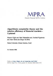
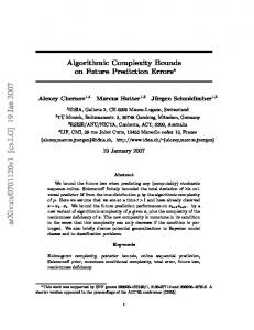
It was shown in [4] that the following version of Not-All-Equal (NAE) satisfying assignment problem is NP-complete. Cubic Monotone NAE (2,3)-Sat. Instance: Set X of variables, collection C of clauses over X such that each clause c ∈ C has | c |∈ {2, 3}, every variable appears in exactly three clauses and there is no negation in the formula. Question: Is there a truth assignment for X such that each clause in C has at least one true literal and at least one false literal? We reduce Cubic Monotone NAE (2,3)-Sat to our problem in polynomial time. Consider an instance Φ, we transform this into a bipartite graph G in polynomial time such that wr(G) = 2 if and only if Φ has an NAE truth assignment. We use three auxiliary gadgets Hc , Ic and B which are shown in Figure 1 and Figure 2.
ac
bc
tc
tc
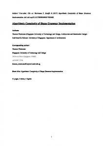
Figure 1: The two gadgets Hc and Ic . The graph Ic is on the right hand side of the figure. Our construction consists of three steps. Step 1. Put a copy of the graph B, a copy of the complete bipartite graph K1,6 and a copy of the complete bipartite graph K3,6 . Step 2. For each clause c ∈ C with | c |= 3, put a copy of the gadget Hc and for each clause c ∈ C with | c |= 2, put a copy of the gadget Ic . Step 3. For each variable x ∈ X, put a vertex x and for each clause c = y ∨z ∨w, where y, z, w ∈ X add the edges ac y, ac z and ac w. Also, for each clause c = y ∨ z, where y, z ∈ X add the edges bc y and bc z. Call the resultant graph G. The degree of every vertex in the graph G is 1 or 3 or 6 and the resultant graph is bipartite. Assume that the graph G can be partitioned into two weakly semiregular graphs G1 and G2 , we have the following lemmas. Lemma 1. The graphs G1 and G2 are (1,3)-graph.
13
Proof of Lemma 1. Without loss of generality, assume that the graph G1 is (α1 , α2 )-graph and the graph G2 is (β1 , β2 )-graph. Since ∆(G) = 6, by attention to the structure of the graph B, with respect to the symmetry, the following cases for (α1 α2 , β1 β2 ) can be considered: (16, 12), (15, 12), (24, 12), (14, 12), (13, 13). The graph G contains a copy of the complete bipartite graph K1,6 , so the case (24,12) is not possible, also, the graph G contains a copy of complete bipartite graph K3,6 , so the cases (16, 12), (15, 12), (14, 12) are not possible. Thus, the graphs G1 and G2 are (1,3)-graph. ♦ Lemma 2. For every vertex v with degree three all edges incident with the vertex v are in one part. Proof of Lemma 2. Since the graphs G1 and G2 are (1,3)-graph, the proof is clear. ♦ Now, we present an NAE truth assignment for the formula Φ. For every x ∈ X, if all edges incident with the vertex x are in the graph G1 , put Γ(x) = true and if all edges incident with the vertex x are in graph G2 , put Γ(x) = f alse. Let c = y ∨ z ∨ w be an arbitrary clause, if all edges ac y, ac z, ac w are in the graph G1 (G2 , respectively), then by the construction of the gadget Hc , the degree of the vertex tc in the graph G2 (G1 , respectively) is at least 5 (5, respectively). This is a contradiction. Similarly, let c = y ∨ z be an arbitrary clause, if all edges bc y, bc z are in the graph G1 (G2 , respectively), then by the construction of Ic , the degree of the vertex tc in the graph G2 (G1 , respectively) is 6. This is a contradiction. Hence, Γ is an NAE satisfying assignment. On the other hand, suppose that Φ is NAE satisfiable with the satisfying assignment Γ : X → {true, f alse}. For every variable x ∈ X, put all edges incident with the the vertex x in G1 if and only if Γ(x) = true. By this method, one can show that the graph G can be partitioned into two weakly semiregular subgraphs. This completes the proof.
v
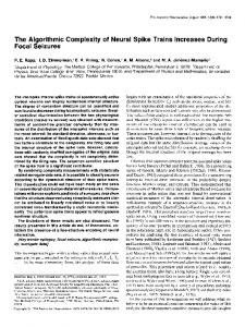
Figure 2: The two gadgets P and B. The graph B is on the right hand side of the figure.
7
Proof of Theorem 3
(i) Any subgraph of a tree is a forest, so in every decomposition of a tree T into some semiregular ) subgraphs, each subgraph is a (1,2)-forest. Thus, sr(T ) ≥ ⌈ ∆(T 2 ⌉. For every bipartite graph ′ H, we have χ (H) = ∆(H) (see for example [46]). Assume that f : E(T ) → {1, . . . , ∆(T )} is a ) proper edge coloring for T . The following partition is a decomposition of T into ⌈ ∆(T 2 ⌉ semiregular 14
subgraphs. ) ⌉ ⌈ ∆(T 2
E(T ) =
[
{e : f (e) = i or f (e) = i + ⌈
i=1
∆(T ) ⌉}. 2
This completes the proof. (ii) Let G be an arbitrary graph. By Vizing’s theorem [45], the edge chromatic number of a graph G is equal to either ∆(G) or ∆(G) + 1. The following partition is a decomposition of G into ′ ⌈ χ (G) 2 ⌉ semiregular subgraphs. ⌈χ
E(G) =
′ (G)
2 [
⌉
{e : f (e) = i or f (e) = i + ⌈
i=1
χ′ (G) ⌉}. 2
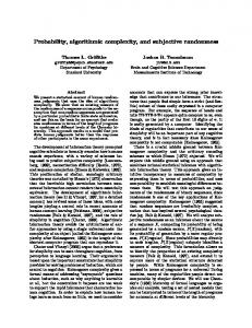
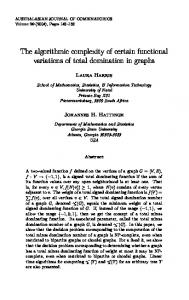
⌉ semiregular subgraphs. So the graph G can be partitioned into ⌈ ∆(G)+1 2 (iii) We use a reduction from the following NP-complete problem [4]. Cubic Monotone NAE (2,3)-Sat. Instance: Set X of variables, collection C of clauses over X such that each clause c ∈ C has | c |∈ {2, 3}, every variable appears in exactly three clauses and there is no negation in the formula. Question: Is there a truth assignment for X such that each clause in C has at least one true literal and at least one false literal? We reduce Cubic Monotone NAE (2,3)-Sat to our problem in polynomial time. Consider an instance Φ, we transform this into a bipartite graph G with ∆(G) ≤ 6 in polynomial time such that sr(G) = 2 if and only if Φ has an NAE truth assignment. We use three auxiliary gadgets Dc , Fc and P which are shown in Figure 3 and Figure 2.
bc
ac
tc
tc
Figure 3: The two auxiliary gadgets Fc and Dc . Dc is on the right hand side of the figure. Our construction consists of three steps. Step 1. Put a copy of the graph P. 15
Step 2. For each clause c ∈ C with | c |= 3, put a copy of the gadget Fc and for each clause c ∈ C with | c |= 2, put a copy of the gadget Dc . Step 3. For each variable x ∈ X, put a vertex x and for each clause c = y ∨z ∨w, where y, z, w ∈ X add the edges ac y, ac z and ac w. Also, for each clause c = y ∨ z, where y, z ∈ X add the edges bc y and bc z. Call the resultant graph G. The degree set of the graph G is {2, 3, 4, 6} and the graph is bipartite. Assume that G can be partitioned into two semiregular graphs G1 and G2 , we have the following lemmas. Lemma 3. The graphs G1 and G2 are (2,3)-graph. Proof of Lemma 3. Without loss of generality assume that G1 is (α − 1, α)-graph such that ∆(G1 ) = α and G2 is (β − 1, β)-graph such that ∆(G2 ) = β. In the graph G any vertex of degree six has a neighbor of degree three, Thus, α 6= 6 and β 6= 6. Also, there is no vertex of degree five, and any neighbor of each vertex of degree six has degree three, so we can assume that α 6= 5 and β 6= 5. In the graph P, the degree of the vertex v is four and the degree of each of its neighbor is two (note that the graph G contains a copy of the graph P). Thus, by the structure of P and since the graph G contains a vertex of degree six, we have α 6= 4 and β 6= 4. On the other hand, since ∆(G) = 6, we have α = β = 3. Hence, the graphs G1 and G2 are (2,3)-graph. ♦ Lemma 4. For every vertex z with degree three or two all edges incident with the vertex z are in one part. Proof of Lemma 4. Since the graphs G1 and G2 are (2,3)-graph, the proof is clear. ♦ Now, we present an NAE truth assignment for the formula Φ. For every x ∈ X, if all edges incident with the vertex x are in G1 , put Γ(x) = true and if all edges incident with the vertex x are in G2 , put Γ(x) = f alse. Let c = y ∨ z ∨ w be an arbitrary clause, if all edges ac y, ac z, ac w are in G1 (G2 , respectively), then by the construction of the gadget Fc and Lemma 4, the degree of the vertex tc in the graph G2 (G1 , respectively) is 4 (4, respectively). This is a contradiction. Similarly, let c = y ∨ z be an arbitrary clause, if all edges bc y, bc z are in G1 (G2 , respectively), then by the construction of the gadget Dc , the degree of the vertex tc in the graph G2 (G1 , respectively) is 4. This is a contradiction. Hence, Γ is an NAE satisfying assignment. On the other hand, suppose that Φ is NAE satisfiable with the satisfying assignment Γ : X → {true, f alse}. For every variable x ∈ X, put all edges incident with the the vertex x in G1 if and only if Γ(x) = true. By this method, it is easy to show that G can be partitioned into two semiregular subgraphs. This completes the proof.
8
Proof of Theorem 4
Let G be a graph. We say that an edge-labeling ℓ : E(G) → N is an additive vertex-colorings if and only if for each edge uv, the sum of labels of the edges incident to u is different from the sum 16
of labels of the edges incident to v. It was shown that determining whether a given 3-regular graph G has an edge-labeling which is an additive vertex-coloring from {1, 2} is NP-complete [3]. For a given 3-regular graph G, it is easy to see that G has an edge-labeling which is an additive vertexcoloring from {1, 2} if and only if the edge set of G can be partitioned into at most two locally irregular subgraphs. Thus, determining whether a given 3-regular graph G can be decomposed into two locally irregular subgraphs is NP-complete [3]. We will reduce this problem to our problem. Let G be a 3-regular graph. We construct a graph G′ such that G can be partitioned into two locally irregular subgraphs if and only if G′ can be partitioned into 2 subgraphs, such that each S8 subgraph is locally irregular or weakly semiregular. Let G′ = G ∪ C4 ∪ P5 ∪ K9,9 i=4 K1,i . The degree set of G′ is D = {j : 1 ≤ j ≤ 9}, so |D| ≥ 9, thus G′ cannot be partitioned into two weakly semiregular subgraphs. Now, assume that G′ can be partitioned into two subgraphs I and R such that I is locally irregular and R is (α, β)-graph. The graph G′ contains a copy of C4 , thus 2 ∈ {α, β}. Also, G′ contains a copy of P5 , thus 1 ∈ {α, β}. Hence R is a (1, 2)-graph. Note that K9,9 cannot be partitioned into two subgraphs I and R such that I is locally irregular and R is (1, 2)-graph. Thus, G′ cannot be partitioned into two subgraphs I and R such that I is locally irregular and R is weakly semiregular. On the other hand, it is easy to see that the graph S8 C4 ∪ P5 ∪ K9,9 i=4 K1,i can be partitioned into two locally irregular subgraphs. Therefore, G can be partitioned into two locally irregular subgraphs if and only if G′ can be partitioned into 2 subgraphs, such that each subgraph is locally irregular or weakly semiregular. This completes the proof.
9
Proof of Theorem 5
(i) Let ǫ > 0 be a fixed number and G be a 3-regular graph with sufficiently large number of vertices in terms of ǫ. Construct the graph H from the graph G by replacing every edge ab of G by a copy of the gadget I(a, b) which is shown in Fig. 4. It was shown that it is NP-complete to determine whether the edge chromatic number of a cubic graph is three [30]. Assume that the number of vertices in the graph H is n. We show that if χ′ (G) = 3 then rep(H c ) ≤ (1 + ǫ)( n2 )3 and if χ′ (G) > 3 then rep(H c ) ≥ ( n2 )4 , consequently, there is no polynomial time θ-approximation algorithm for computing rep(Ac ) when ( n2 )4 n n = > (1 − ǫ) = θ. (1 + ǫ)( n2 )3 2(1 + ǫ) 2 By the structure of the gadget I(a, b), the graph H is 3-regular and triangle-free, also by the structure of H, χ′ (G) = χ′ (H). Note that if H is triangle-free then rep(H c ) is square free. Qd Let rep(H c ) = i=1 pi , where for each i, i = 1, . . . , d, pi is a prime number. Assume that r : V (H c ) −→ Zrep(H c ) is a representation for H c . For each vertex v of H c define a d-triple Qd (rv1 , . . . , rvd ) ∈ i=1 Zpi such that rvi = (r(v) mod pi ). By the definition of the function r, vw is an i edge in H if and only if there exists an index i such that rvi = rw . For each edge e = xy of H, define i i S(e) = {i : rx = ry }. So for each edge e, S(e) is non-empty and since the graph H is triangle-free, for every two incident edges e and e′ we have S(e) ∩ S(e′ ) = ∅. Let c : E(H) −→ {1, . . . , d} be a 17
function such that c(e) = min S(e). It is clear that c is a proper edge coloring for the graph H. So d ≥ χ′ (H)
(2)
a
b
Figure 4: The auxiliary graph I(a, b). Define Mi = {e ∈ E(H), i ∈ S(e)} for every i, 1 ≤ i ≤ d. The set Mi contains all edges of the graph H like e = vu such that v and u have a same i-th component. Since the graph H is triangle-free, it follows that the set of edges Mi is a matching. Also, each z ∈ Zpi appears at most 2 times as the i-th component of vertices in the graph H. Also, each vertex of H which is not adjacent to any vertex of Mi , has a unique i-th component. For each i denote the number of edges of Mi by mi (note that |V (H)| = |V (H c )| = n). We have: pi ≥ mi + (n − 2mi ) = n − mi Also, since every matching has at most
n 2
(3)
edges, it follows that pi ≥
n 2
(4)
Now, let χ′ (H) = 3 and f : E(H) −→ {1, 2, 3} be a proper edge coloring of H. The edges of H can be partitioned into three perfect matchings f1 , f2 and f3 , where fi = {e : f (e) = i}. Without n loss of generality for each i, i = 1, 2, 3, assume that fi = {e1i , . . . , ei2 }. It follows from the prime number theorem that for any real α > 0 there is a n0 > 0 such that for all n′ > n0 there is a prime p such that n′ < p < (1+α)n′ (see [29] page 494). Thus for a sufficiently 1 large number n, there are three prime numbers p1 , p2 , p3 such that n2 ≤ p1 < p2 < p3 < n2 (1 + ǫ) 3 . β γ For every vertex v of the graph H, call the edges incident with the vertex v, eα 1 , e2 and e3 and let ψ : V (H c ) −→ Zp1 p2 p3 be a function such that ψ(v) = (α, β, γ). Clearly, this is a representation, so rep(H c ) ≤ p1 p2 p3 < (1 + ǫ)( n2 )3 . On the other side, assume that χ′ (G) > 3, so χ′ (H) > 3. Thus, we have:
rep(H c ) =
d Y
pi
≥
i=1 4 Y
pi
By Equation 2,
n ≥ ( )4 2
By Equation 4,
i=1
18
This completes the proof. (ii) Let Gc be a triangle-free r-regular graph. By Vizing’s theorem [45], the chromatic index of Gc is equal to either ∆(Gc ) or ∆(Gc ) + 1. Thus, for every r-regular graph Gc , r ≤ χ′ (Gc ) ≤ r + 1. Therefore, the set of edges of Gc can be partitioned into r + 1 matchings M1 , . . . , Mr+1 . By an argument similar to the proof of part (i), we have:
rep(G) ≤ (1 + ǫ)
r+1 Y
(n − |Mi |)
i=1
≤ (1 + ǫ)(n −
rn )r+1 2(r + 1)
n ≤ (1 + ǫ)e( )r+1 2
By Equation 3, By inequality (1 +
1 x ) < e, x
On the other hand n rep(G) ≥ ( )r . 2 Therefore we have a polynomial time (1 + ǫ) 2e n approximation algorithm for computing rep(G).
10 10.1
Concluding remarks and future work Trees
We proved that for every tree T , wr(T ) ≤ 2 log2 ∆(T ) + O(1). On the other hand, there are infinitely many values of ∆ for which the tree T might be chosen so that wr(T ) ≥ log3 ∆(T ). Finding the best upper bound for trees can be interesting. Problem 1. Find the best upper bound for the weakly semiregular numbers of trees in terms of the maximum degree. We proved that there is an O(n2 ) time algorithm to determine whether the weakly semiregular number of a given tree is two. Also, if c is a constant number, then there is a polynomial time algorithm to determine whether the weakly semiregular number of a given tree is at most c. However, one further step does not seem trivial. Is there any polynomial time algorithm to determine the weakly semiregular number of trees? Problem 2. Is there any polynomial time algorithm to determine the weakly semiregular number of trees? In this work we present an algorithm with running time O(n2 ) to determine whether the weakly semiregular number of a given tree is at most two. Is there any algorithm with running time O(n lg n) for this problem? 19
Problem 3. Is there any algorithm with running time o(n2 ) for determining whether the weakly semiregular number of a given tree is at most two?
10.2
Planar graphs
Balogh et al. proved that a planar graph can be partitioned into three forests so that one of the forests has maximum degree at most 8 [10]. On the other hand, we proved that for every tree T , wr(T ) ≤ 2 log2 ∆(T )+O(1). Thus, for every planar graph G, we have wr(G) ≤ 4 log2 ∆(G)+O(1). Also, it was shown that every planar graph with girth g ≥ 6 has an edge partition into two forests, one having maximum degree at most 4 [28]. Thus, for every planar graph G with girth g ≥ 6, we have wr(G) ≤ 2 log2 ∆(G) + O(1). Finding a good upper bound for all planar graphs can be interesting. Problem 4. Is this true ”For every planar graph G, we have wr(G) ≤ 2 log2 ∆(G) + O(1)”?
10.3
Representation Number
In this work, we proved that if NP 6= P, then for any ǫ > 0, there is no polynomial time (1 − ǫ) n2 approximation algorithm for the computation of representation number of regular graphs with n vertices. In 2000 it was shown by Evans, Isaak and Narayan [26] that if n, m ≥ 2, then rep(nKm ) = pi pi+1 . . . pi+m−1 where pi is the smallest prime number greater than or equal to m if and only if there exists a set of n − 1 mutually orthogonal Latin squares of order m. It is interesting to investigate what our result implies about the Orthogonal Latin Square Conjecture (There exists n − 1 mutually orthogonal Latin squares of order n if and only if n is a prime power). That is, can our reduction be extended from regular graphs to just nKm .
11
Acknowledgments
The authors would like to thank the anonymous referees for their useful comments which helped to improve the presentation of this paper.
References [1] A. Ahadi and A. Dehghan. The inapproximability for the (0, 1)-additive number. Discrete Math. Theor. Comput. Sci., 17(3):217–226, 2016. [2] A. Ahadi, A. Dehghan, M. Kazemi, and E. Mollaahmadi. Computation of lucky number of planar graphs is NP-hard. Inform. Process. Lett., 112(4):109––112, 2012. [3] A. Ahadi, A. Dehghan, and M.-R. Sadeghi. Algorithmic complexity of proper labeling problems. Theoret. Comput. Sci., 495:25–36, 2013. 20
[4] A. Ahadi, A. Dehghan, and M.-R. Sadeghi. On the complexity of deciding whether the regular number is at most two. Graphs Combin., 31(5):1359–1365, 2015. [5] A. Ahadi, A. Dehghan, M.-R. Sadeghi, and B. Stevens. Partitioning the edges of graph into regular, locally regular and/or locally irregular subgraphs is hard no matter which you choose. Submitted, 2015. [6] R. Akhtar, A. B Evans, and D. Pritikin. Representation numbers of complete multipartite graphs. Discrete Math., 312(6):1158–1165, 2012. [7] R. P. Anstee. An algorithmic proof of tutte’s f-factor theorem. J. Algorithms, 6(1):112–131, 1985. [8] C. Balbuena, D. Gonz´ alez-Moreno, and X. Marcote. On the connectivity of semiregular cages. Networks, 56(1):81–88, 2010. [9] C. Balbuena, X. Marcote, and D. Gonz´alez-Moreno. Some properties of semiregular cages. Discrete Math. Theor. Comput. Sci., 12(5):125–138, 2010. [10] J. Balogh, M. Kochol, A. Pluh´ ar, and X. Yu. Covering planar graphs with forests. J. Combin. Theory Ser. B, 94(1):147–158, 2005. [11] E. Barme, J. Bensmail, J. Przyby?o, and M. Wo?niak. On a directed variation of the 1-2-3 and 1-2 Conjectures. Discrete Appl. Math., 217(part 2):123–131, 2017. [12] O. Baudon, J. Bensmail, J. Przybylo, and M. Wo´zniak. On decomposing regular graphs into locally irregular subgraphs. European J. Combin., 49:90–104, 2015. [13] O. Baudon, J. Bensmail, and E. Sopena. On the complexity of determining the irregular chromatic index of a graph. J. Discrete Algorithms, 30:113–127, 2015. [14] P. Bennett, A. Dudek, A. Frieze, and L. Helenius. Weak and strong versions of the 1-2-3 conjecture for uniform hypergraphs. Electron. J. Combin., 23(2):Paper 2.46, 21, 2016. [15] J. Bensmail. Partitions and decompositions of graphs. PhD thesis, Universit´e de Bordeaux, 2014. [16] J. Bensmail, M. Merker, and C. Thomassen. Decomposing graphs into a constant number of locally irregular subgraphs. European J. Combin., 60:124–134, 2017. [17] J. Bensmail and B. Stevens. Decomposing graphs into locally irregular subgraphs: allowing k2’s helps a lot. Bordeaux Graph Workshop, France, page 103, 2014. [18] J. Bensmail and B. Stevens. Edge-partitioning graphs into regular and locally irregular components. Discrete Math. Theor. Comput. Sci., 17(3):43–58, 2016. [19] F. R. K. Chung. On the decomposition of graphs. SIAM J. Algebraic Discrete Methods, 2(1):1–12, 1981.
21
[20] A. Dehghan and M. Mollahajiaghaei. On the algorithmic complexity of adjacent vertex closed distinguishing colorings number of graphs. Discrete Appl. Math., 218:82–97, 2017. [21] A. Dehghan and M.-R. Sadeghi. Colorful edge decomposition of graphs: Some polynomial cases. Discrete Appl. Math., 2016, http://dx.doi.org/10.1016/j.dam.2016.10.019. [22] A. A. Diwan, J. E. Dion, D. J. Mendell, M. J. Plantholt, and S. K. Tipnis. The complexity of P4 -decomposition of regular graphs and multigraphs. Discrete Math. Theor. Comput. Sci., 17(2):63–75, 2015. [23] Dorit Dor and Michael Tarsi. Graph decomposition is NP-complete: a complete proof of Holyer’s conjecture. SIAM J. Comput., 26(4):1166–1187, 1997. [24] P. Erd˝ os and A. B. Evans. Representations of graphs and orthogonal latin square graphs. J. Graph Theory, 13(5):593–595, 1989. [25] A. B. Evans, G. H. Fricke, C. C. Maneri, T. A. McKee, and M. Perkel. Representations of graphs modulo n. J. Graph Theory, 18(8):801–815, 1994. [26] A. B. Evans, G. Isaak, and D. A. Narayan. Representations of graphs modulo n. Discrete Math., 223(1-3):109–123, 2000. [27] A. Ganesan and R. R. Iyer. The regular number of a graph. J. Discrete Math. Sci. Cryptogr., 15(2-3):149–157, 2012. [28] D. Gon¸calves. Covering planar graphs with forests, one having bounded maximum degree. J. Combin. Theory Ser. B, 99(2):314–322, 2009. [29] G. H. Hardy and E. M. Wright. An introduction to the theory of numbers. The Clarendon Press, Oxford University Press, New York, fifth edition, 1979. [30] I. Holyer. The NP-completeness of edge-coloring. SIAM J. Comput., 10(4):718–720, 1981. [31] I. Holyer. The NP-completeness of some edge-partition problems. 10(4):713–717, 1981.
SIAM J. Comput.,
[32] D. Kiani and M. Mollahajiaghaei. On the unitary Cayley graphs of matrix algebras. Linear Algebra Appl., 466:421–428, 2015. [33] D. G. Kirkpatrick and P. Hell. On the complexity of general graph factor problems. SIAM J. Comput., 12(3):601–609, 1983. [34] V. R. Kulli, B. Janakiram, and R. R. Iyer. Regular number of a graph. J. Discrete Math. Sci. Cryptography, 4(1):57–64, 2001. [35] Charles C. Lindner, E. Mendelsohn, N. S. Mendelsohn, and Barry Wolk. Orthogonal Latin square graphs. J. Graph Theory, 3(4):325–338, 1979. [36] B. Luˇzar, J. Przybylo, and R. Sot´ak. New bounds for locally irregular chromatic index of bipartite and subcubic graphs. arXiv preprint arXiv:1611.02341, 2016. 22
[37] D. Narayan. An upper bound for the representation number of graphs with fixed order. Integers, 3(4):A12, 2003. [38] D Narayan and J. Urick. Representations of split graphs, their complements, stars, and hypercubes. Integers, 7(13):A9, 2007. [39] J. Petersen. Die theorie der regul¨ aren graphs. Acta Mathematica, 15(1):193–220, 1891. [40] M. D. Plummer. Graph factors and factorization: 1985–2003: a survey. Discrete Math., 307(7-8):791–821, 2007. [41] J. Przybylo. On decomposing graphs of large minimum degree into locally irregular subgraphs. Electron. J. Combin., 23(2):Paper 2.31, 13, 2016. [42] J. Przybylo and M. Wo´zniak. On a 1, 2 conjecture. Discrete Math. Theor. Comput. Sci., 12(1):101–108, 2010. [43] B. Seamone. The 1-2-3 conjecture and related problems: a survey. arXiv:1211.5122. [44] B. Seamone and B. Stevens. Sequence variations of the 1-2-3 conjecture and irregularity strength. Discrete Math. Theor. Comput. Sci., 15(1):15–28, 2013. [45] V. G. Vizing. On an estimate of the chromatic class of a p-graph. Diskret. Analiz No., 3:25–30, 1964. [46] D. B. West. Introduction to graph theory. Prentice Hall Inc., Upper Saddle River, NJ, 1996.
23