Algorithmic complexity theory and the relative efficiency of financial ...

M PRA Munich Personal RePEc Archive

Algorithmic complexity theory and the relative efficiency of financial markets Updated Ricardo Giglio and Raul Matsushita and Annibal Figueiredo and Iram Gleria and Sergio Da Silva Federal University of Santa Catarina, Brazil

16. October 2008

Online at http://mpra.ub.uni-muenchen.de/11150/ MPRA Paper No. 11150, posted 19. October 2008 06:48 UTC

Algorithmic complexity theory and the relative efficiency of financial markets Ricardo GIGLIO1, Raul MATSUSHITA2, Annibal FIGUEIREDO3, Iram GLERIA4 and Sergio DA SILVA1 1

Department of Economics, Federal University of Santa Catarina, 88049970 Florianopolis SC, Brazil Department of Statistics, University of Brasilia, 70910900 Brasilia DF, Brazil 3 Institute of Physics, University of Brasilia, 70910900 Brasilia DF, Brazil 4 Institute of Physics, Federal University of Alagoas, 57072970 Maceio AL, Brazil 2

PACS 89.65.Gh – First pacs description PACS 89.20.-a – Second pacs description Abstract – Financial economists usually assess market efficiency in absolute terms. This is to be viewed as a shortcoming. One way of dealing with the relative efficiency of markets is to resort to the efficiency interpretation provided by algorithmic complexity theory. We employ such an approach in order to rank 36 stock exchanges and 20 US dollar exchange rates in terms of their relative efficiency.

Introduction – Informational efficiency of financial markets is a central, hot topic in finance. It is meant that if price changes fully incorporate the information in possession of all market participants such changes are unpredictable; the market in question is then said to be information efficient. Early empirical observations of the statistical properties of prices [1], [2] detected a Brownian motion. In an efficient market populated by rational agents if the price is properly anticipated then it must fluctuate randomly [3]. Such a stochastic process resembles a probabilistic model of a fair game, one in which gains and losses cancel each other out. When informed traders move to take advantage of their information, the price will move by an amount and in the direction that eliminates this advantage. As a result, there is an association between the unanticipated information obtained by the informed traders and the consequent movement of market prices. The uninformed traders can then infer from an observed price increase that some traders in the market have favorable information about the asset. Information is not wasted, and the price is a sufficient statistic for all relevant information in possession of all traders [4], [5], [6]. Thus the efficient market theory [7] is the notion that prices in financial markets promptly adjust to reflect information. After presenting an overview of market efficiency in their

classic financial econometrics textbook, Campbell and coauthors [8] observed that (p. 24) the notion of relative efficiency, i.e. the efficiency of one market measured against another may be a more useful concept than the all-or-nothing (absolute) view taken by much of the traditional efficiency market literature. They made an analogy with physical systems that are usually given an efficiency rating based on the relative proportion of energy converted to work. The efficient market is an idealized concept that is unattainable, but that serves as a fundamental benchmark for measuring relative efficiency. Indeed, one must regard the efficient market hypothesis as a limiting case. In practice, prices reflect only the information for which the acquisition costs cannot outweigh the benefits. There are also transaction costs. Moreover, information may not be widely disseminated and thus reflected in prices. Following the arrival of new information, market participants may diverge from one another in how they think it will impact prices; in other words, expectations are heterogeneous. Residual inefficiencies are always present in actual markets. Such inefficiencies can introduce artificial patterns and then redundant information in real-world financial price series. Thus it is inappropriate to assess whether a given actual market is efficient or not. A proper definition of efficiency has to measure to what extent one

market departs from the idealized efficient market. Algorithmic complexity theory makes a connection between the efficient market hypothesis and the unpredictable character of asset returns because a time series that has a dense amount of non-redundant information (such as that of the idealized efficient market) exhibits statistical features that are almost indistinguishable from those observed in a time series that is random [9]. As a result, measurements of the deviation from randomness provide a tool to assess the relative efficiency of a given market. Because algorithmic complexity theory cannot discriminate between trading on noise and trading on information, it detects no difference between a time series conveying a large amount of non-redundant information and a pure random process. We adopt such an approach. Considering financial markets as complex systems is already common in econophysics [10], [11]. Sharing such a perspective, here we will present a method that allows us to rank stock exchanges and currencies in terms of their relative efficiency. The absolute efficiency of stock markets has been investigated in a huge number of papers [12], [7], but we could track only three previous attempts similar to ours to deal with their relative efficiency. Shmilovici and colleagues [13] provide a test based on the insight that the compression of the efficient market time series is not possible since there are no patterns. In that case, “stochastic complexity” is highest. The stochastic complexity of a time series is a measure of the number of binary digits needed to represent and reproduce the information in the time series. The authors use the Rissanen context tree algorithm to track patterns and then compress the series of 13 stock exchange indices as well as the stock prices of the companies listed on the Tel-Aviv 25. Also, Chen and Tan [14] suggested an approach that was proved to be one particular case of that in Shmilovici et al. And Oh and coauthors [15] explicitly addressed the relative efficiency of currency markets using a tool called the approximate entropy statistic [16]. The tool aimed at tracking similar subsets in a time series. The approximate

entropy statistic is strongly alignmentdependent, however, in that two parameters (lag length and the similarity criterion) must be specified a priori [17] (see also [18]). Next section will show our distinct perspective applied to a larger data base along with a simpler methodology that is based straightforwardly on the Lempel-Ziv (“deterministic”) complexity index. Lempel-Ziv algorithmic complexity – Shannon entropy of information theory implies that a genuinely random series is the limiting case where its expected information content is maximized, in which case there is maximum uncertainty and no redundancy in the series. The algorithmic (Kolmogorov) complexity of a string is given by the length of the shortest computer program that can produce the string. The shortest algorithm cannot be computable, however. Yet there are several ways to circumvent this problem. Lempel and Ziv [19] suggest a useful measure that does not rely on the shortest algorithm. Kaspar and Schuster [20] provide an easily calculable measure of the Lempel-Ziv index which runs as follows. A program first either inserts a new digit into the binary string S = s1 ,… , sn or copies the new digit to S . The program then reconstructs the entire string up to the digit sr < sn that has been newly inserted. Digit sr does not come from the substring s1 ,… , sr −1 ; otherwise, sr could simply be copied from s1 ,… , sr −1 . To learn whether the rest of S can be reconstructed by either simply copying or inserting new digits we take sr +1 , and then check whether this digit belongs to one of the substrings of S , in which case it can be obtained by simply copying it from S . If sr +1 can indeed be copied the routine goes on until a new digit (which once again needs to be inserted) appears. The number of newly inserted digits plus one (if the last copy step is not followed by inserting a digit) gives the complexity measure c of the string S . As an illustration, consider the following three strings of 10 binary digits each. A 0000000000

B 0101010101 C 0110001001 At first sight one might correctly guess that A is less random so that A is less complex than B, which in turn is less complex than C. The complexity index c agrees with such an intuition. For the string A one has only to insert the first zero and then rebuild the entire string by copying this digit; thus c = 2 , where c is the number of steps necessary to create a string. For the string B one has to additionally insert digit 1 and then copy the substring 01 to reconstruct the entire string; thus c = 3 . For the string C one has to further insert 10 and 001, and then copy 001; thus c =5. A genuinely random string asymptotically approaches its maximum complexity r as its length n grows following the rule lim c = r = logn2 n [20]. One may thus n →∞

compute a positive finite normalized complexity index LZ = cr to get the complexity of a string relative to that of a genuinely random one. Under the Lempel and Ziv [19] broad definition of complexity almost all sequences of sufficiently large length are found to be complex. To get a useful measure of complexity, they then take a De Bruijn sequence, which is commonly considered as a good finite approximation of a complex sequence [19]. After proving that the De Bruijn sequence is indeed complex according to their definition, and that its complexity index cannot be less than one, they decided to take it as a benchmark against which other sequences could be compared. Thus a finite sequence with a complexity index greater than one is guaranteed to be more complex than (or at least as complex as) a De Bruijn sequence of same size. Note then that the LZ index is not an absolute measure of complexity (which is perhaps nonexistent); nor is the index ranged between zero and one. Here we consider sliding time windows, calculate the LZ index for every window, and then get the average. For instance, for a time series of 2,000 data points and a chosen time window of 1,000 observations we first compute the LZ index of the window from 1 to 1,000, then the index of the window from 2 to 1,001, and so on, up to

the index of the window from 1,001 to 2,000. Then we take the average of the indices. Efficiency can also be thought of as lack of autocorrelation. The LZ complexity can also capture that, and is general enough to encompass Markov processes. In a sense, the LZ index provides a statistic that is more basic than those produced by autoregressive processes of any order. If a time series is autocorrelated we expect it to present more patterns and accordingly to have lower complexity than an independent one. That the LZ complexity measure can also capture this feature can be seen in the example of an unfair coin, whose probability distribution of the current value is dependent on the previous one with probability p. If p = ½ the process collapses to that of the fair coin with no memory (i.e. an independent process); if either p = 0 or p = 1 the current value is perfectly predictable from past observation, i.e. the process is totally dependent. We reckoned the LZ index of the sequences generated by the unfair coin for different probabilities only to find a parabola-shaped curve (not shown). This means that maximum complexity is reached if p = ½, and lack of complexity obtains as the probability is either 0 or 1. Some applications of the LZ index in literature include the following. Use for DNA sequencing in order to reconstruct the phylogenetic tree of several species of placental mammals [21]. Analysis of the complexity of the heart rate variability signals to identify intrauterine growth-restricted fetuses [18], and even identification of temporal complexity in short sequences of musical rhythms [22]. Data and analysis – We collected seven years of daily data from July 2000 to July 2007 (2,000 observations) from 36 stock exchange indices (Table 1), and 20 US dollar exchange rates (Table 2). The source was Yahoo Finance and EconStats. Analysis was performed with the returns of the raw series. The return series were coded as ternary strings as follows [13]. Assuming a stability basin b for a return observation ρt , a data point dt of the ternary

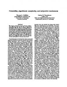
string was coded as dt = 0 if ρt ≤ −b , dt = 1 if ρt ≥ +b , and dt = 2 if − b < ρt < +b . The series would have become binary if we had shrunk the stability basin to the attractor zero, i.e. b = 0 ; yet we assumed b = 0.0025 following Shmilovici et al.. We checked for the effects of changing b only to realize that the rankings did not alter too much; yet more research is needed to consider a more sophisticated analysis in the choice of b . As an illustration, we take five daily percentage returns of the S&P 500 and compare them with b = 0.25%. From 18 to 22 June 2007 the percentage returns were, respectively, 0.652, –0.1226, 0.1737, –1.381, and 0.6407. Thus the trading week was coded as 12201. Figure 1 shows the evolution of the index using 1,000 sliding windows for (a) a computer-generated pseudo-random series (average LZ from all the 1,000 windows = 1.0180), (b) returns of the Dow Jones (average LZ = 1.0201), (c) returns of the Shanghai Composite (average LZ index = 1.0032), and (d) returns of the Karachi 100 (average LZ index = 0.9918). Table 1 shows the average LZ indices and variances for all the stock exchanges. As can be seen, all the series seem to be very complex. They look more like the genuinely random series than the totally redundant, perfectly predictable series. Based on the discussion presented above we considered LZ = 1 as a threshold, counted the number of occurrences where the LZ index was caught above one, and then considered that as a measure of relative efficiency. For the pseudo-random series the LZ = 1 threshold was surpassed 98.8% of the times; thus we say that it is 98.8% efficient. (Of course, the efficiency measure of a pseudo-random series will vary depending on how such a series is generated.) The Dow Jones, Shanghai Composite, and Karachi 100 were found to be, respectively, 95.4%, 49.5%, and 23.7% efficient. Note that the Dow Jones series looks like the pseudo-random series of our example. Table 1 shows the measures for all the stock exchanges. As can be seen, the S&P 500 even beats our pseudo-random series. By contrast, the Colombo Stock Exchange was found to be only 10.5% efficient, which means that stock prices in that market convey

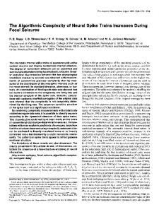
some redundant information. As expected [23], we have found the less developed markets less efficient. Table 2 shows the relative efficiency of selected US dollar exchange rates, whereas Fig. 2 displays the LZ index evolution over the same sliding windows (i.e. 1,000) for the dollar price in terms of (a) pound sterling (average LZ index = 1.0223; 99.81% efficient), (b) euro (average LZ index = 1.0254; 99.45% efficient), (c) Brazilian real (average LZ index = 1.0156; 92.60% efficient), (d) Indian rupee (average LZ index = 0.9958; 43.54% efficient), and (e) Chinese yuan (average LZ index = 0.9266; 17.94% efficient). As for the latter, the initial low complexity of the dollar price in yuan terms in Fig. 2 can be explained by the fact that China’s currency remained pegged to the US dollar from 16 June 1994 to 21 July 2005 [24]. It can be said that generally we have presented a method that deals with the hierarchy of related complex systems. Yet there are other alternative ways of doing such rankings (see [25], [26], [27], and references therein). As a control experiment we considered one such method, namely detrended fluctuation analysis (DFA). Our estimate procedure followed Ref. [25]. (Further details are provided elsewhere [28]). The DFA outperforms the traditional Hurst exponents and other methods designed to track long range memory [25], [29], [30]. The last two columns in Tables 1 and 2 show the average DFA exponents of the 1,000 sliding windows using 5-day sliding steps and a scale range of 100 days. Because our aim was to make a comparison with the LZ index, we considered returns (rather than log returns) and sliding windows of same size (i.e. 1,000) when estimating the DFA exponents. One limitation of such an estimation procedure is that there is a bias introduced into the estimates within each window because returns are sensitive to scale changes. Tables 1 and 2 also show the percentage of the times that the DFA exponent values were caught inside the interval 0.5 ± 0.06. Fig. 3 takes four series to illustrate it. Interval 0.5 ± 0.06 was arbitrarily chosen. We could observe that the ranking varied depending on the interval length (not

shown). This means that such an interval length choice becomes a serious issue in here (see [31]). Overall the stock market indices and exchange rates presented weak long range memory. This finding is consistent with that of high complexity of the series. Also, the indices and exchange rates of developed markets were top ranked. But the matching between the LZ indices and the DFA exponents were not that perfect. This is not so surprising since we have employed an arbitrary stability basin b for the LZ as well as an ad hoc interval length for the DFA. Conclusion – By considering data from 36 stock market indices and 20 US dollar exchange rates, this paper puts forward a method to assess the relative efficiency of financial markets. This is made possible thanks to the efficiency interpretation provided by algorithmic complexity theory. The latter makes a connection between the efficient market hypothesis and the unpredictable character of asset returns. The idealized efficient market generates a time series that has a dense amount of nonredundant information, and thus presents statistical features similar to a genuinely random time series. Physical systems are usually given an efficiency rating based on the relative proportion of energy converted to work. We suggest an analogous efficiency rating based on the relative amount of non-redundant information conveyed by financial prices. The price of the idealized efficient market conveys information that is fully nonredundant; this market is then said to be 100% efficient. Since residual inefficiencies are always present in actual markets one should not expect some of them to be efficient in absolute terms. Yet by considering the random efficient market as a benchmark one can, for instance, say that the S&P 500 is 99.1% efficient whereas the Colombo Stock Exchange is only 10.5% efficient.

*** We are very grateful to two anonymous referees and to the coeditor for useful comments. Financial support from the Brazilian agencies CNPq and CAPES (Procad) is also acknowledged.

REFERENCES [1] BACHELIER M. L., Theorie de la Speculation (Gauthier-Villars, Paris) 1900. [2] FAMA E. F., Journal of Business, 38 (1965) 34. [3] SAMUELSON P. A., Industrial Management Review, 6 (1965) 41. [4] HAYEK F. A., American Economic Review, 35 (1945) 519. [5] GROSSMAN S. J., Journal of Finance, 31 (1976) 573. [6] IVANOV P. C., YUEN A., PODOBNIK B. and LEE, Y., Physical Review E, 69 (2004) 056107. [7] FAMA E. F., Journal of Finance, 25 (1970) 383. [8] CAMPBELL J. Y., LO A.W. and MACKINLAY A. C., The Econometrics of Financial Markets (Princeton University Press, Princeton) 1997. [9] MANTEGNA R. N. and STANLEY H. E., An Introduction to Econophysics: Correlations and Complexity in Finance (Cambridge University Press, Cambridge) 2000. [10] MATIA K., ASHKENAZY Y. and STANLEY H. E., Europhysics Letters, 61 (2003) 422. [11] NASCIMENTO C. M., JUNIOR H. B. N., JENNINGS H. D., SERVA M., GLERIA I. and VISWANATHAN G. M., Europhysics Letters, 81 (2008) 18002. [12] BEECHEY M., GRUEN D. and VICKERY J., Reserve Bank of Australia Research Discussion Paper, No. 2000-01, 2000. [13] SHMILOVICI A., ALON-BRIMER Y. and HAUSER S., Computational Economics, 22 (2003) 273. [14] CHEN S. H. and TAN C. W., Journal of Management and Economics, 3 (1999) 3. [15] OH G., KIM S. and EOM C., Physica A, 382 (2007) 209. [16] PINCUS S., Proceedings of the National Academy of Sciences of the USA, 88 (1991) 2297. [17] RICHMAN J. S. and MOORMAN J.R., American Journal of Physiology, 278 (2000) 2039. [18] FERRARIO M., SIGNORINI M. and MAGENES G., Computers in Cardiology, 32 (2005) 989.

[19] LEMPEL A. and ZIV J., IEEE Transactions on Information Theory, 22 (1976) 75.

[26] MANTEGNA R. N., European Physical Journal B, 11 (1999) 193.

[20] KASPAR F. and SCHUSTER H. G., Physical Review A, 36 (1987) 842.

[27] GLIGOR M. and AUSLOOS M., European Physical Journal B, 63 (2008) 533.

[21] LI B., LI Y. B. and HE H. B., Genomics, Proteomics & Bioinformatics, 3 (2005) 206.

[28] MATSUSHITA R., GLERIA I., FIGUEIREDO A. and DA SILVA S., Physics Letters A, 368 (2007) 173.

[22] SHMULEVICH I. and POVEL D. J., Journal of New Music Research, 29 (2000) 61.

[29] HU K., IVANOV P. C., CHEN Z., CARPENA P. and STANLEY H. E., Physical Review E, 64 (2001) 011114.

[23] PODOBNIK B., FU D., JAGRIC T., GROSSE I. and STANLEY H. E., Physica A, 362 (2006) 465. [24] MATSUSHITA R., FIGUEIREDO A., GLERIA I. and DA SILVA S., Physica A, 378 (2007) 427.

[30] CHEN Z., IVANOV P. C., HU K. and STANLEY H. E., Physical Review E, 65 (2002) 041107. [31] COUILLARD M. and DAVISON M., Physica A, 348 (2005) 404.

[25] XU L., IVANOV P. C., HU K., CHEN, Z., CARBONE, A. and STANLEY H. E., Physical Review E, 71 (2005) 1. Fig. 2: LZ index evolution over 1,000 sliding windows for the dollar price in terms of (a) pound sterling (average LZ index = 1.0223; 99.81% efficient), (b) euro (average LZ index = 1.0254; 99.45% efficient), (c) Brazilian real (average LZ index = 1.0156; 92.60% efficient), (d) Indian rupee (average LZ index = 0.9958; 43.54% efficient), and (e) Chinese yuan (average LZ index = 0.9266; 17.94% efficient).

Fig. 1: LZ index evolution over 1,000 sliding windows for (a) a computer-generated pseudo-random series (average LZ = 1.0180), (b) returns of the Dow Jones (average LZ = 1.0201), (c) returns of the Shanghai Composite (average LZ index = 1.0032), and (d) returns of the Karachi 100 (average LZ index = 0.9918).

Fig. 3: DFA exponent evolution over 1,000 sliding windows for (a) returns of the S&P 500 index (average DFA = 0.4759; 98.3% of the occurrences inside the interval 0.5 ± 0.06), (b) returns of the Karachi 100 (average DFA = 0.5881; 23.3% of the occurrences inside the interval 0.5 ± 0.06), (c) dollar price in pounds (average DFA = 0.5272; 98.6% of the occurrences inside the interval 0.5 ± 0.06), and (d) dollar price in yuans (average DFA = 0.3655; 39.6% of the occurrences inside the interval 0.5 ± 0.06).

Table 1. The relative efficiency of selected stock market indices Stock Exchange

Country

S&P 500

USA

DAX 30

GER

Nikkei 225

JPN

All Ordinaries

AUS

ATX

AUT

Dow Jones

USA

Korea Composite

KOR

Tel-Aviv 100

ISR

Hang Seng

HKG

Straits Times

SIN

CAC 40

FRA

Helsinki General

FIN

Kuala Lumpur SE

MAS

FTSE 100

UK

Prague X

CZE

Bel 20

BEL

IBC

VEN

Madrid General

ESP

Swiss Market

SUI

Nasdaq Composite Amsterdam EX

USA NED

Bovespa

BRA

IPC

MEX

Merval

ARG

Jakarta Composite

IDN

Istanbul 100

TUR

Moscow Times

RUS

Copenhagen

DEN

Athex Composite

GRE

Bombay SE

IND

Taiwan Weighted

TPE

Shanghai Composite

CHN

Philippines

PHI

Lima General

PER

Karachi 100

PAK

Colombo SE

SRI

Average and Variance of the LZ Index 1.0232 (0.0001) 1.0257 (0.0002) 1.0432 (0.0002) 1.0246 (0.0002) 1.0173 (0.0001) 1.0201 (0.0001) 1.0163 (0.0001) 1.0187 (0.0001) 1.0151 (0.0001) 1.0153 (0.0001) 1.0138 (0.0002) 1.0149 (0.0048) 1.0158 (0.0003) 1.0106 (0.0005) 1.0139 (0.0002) 1.0118 (0.0000) 1.0110 (0.0003) 1.0201 (0.0001) 1.0101 (0.0003) 1.0080 (0.0001) 1.0100 (0.0003) 1.0127 (0.0002) 1.0060 (0.0001) 1.0050 (0.0003) 1.0054 (0.0002) 1.0085 (0.0004) 1.0050 (0.0001) 1.0025 (0.0002) 1.0048 (0.0001) 1.0010 (0.0002) 1.0006 (0.0004) 1.0032 (0.0014) 0.9987 (0.0002) 0.9903 (0.0001) 0.9918 (0.0001) 0.9795 (0.0004)

Relative Efficiency*, % 99.1 98.4 98.2 97.8 97.4 95.4 94.9 92.9 91.5 90.3 88.4 88.4 88 86.6 81 80.4 79.9 79.3 78.4 75.4 74.4 67.8 64 62.9 62.1 61.3 59.2 58.7 56.9 53.3 50.3 49.5 43.1 37.9 23.7 10.5

Average and Variance of the DFA Exponent 0.4759 (0.0004) 0.4794 (0.0006) 0.4626 (0.0007) 0.5420 (0.0004) 0.5556 (0.0006) 0.4990 (0.0004) 0.4663 (0.0003) 0.5395 (0.0010) 0.5225 (0.0007) 0.4894 (0.0009) 0.4402 (0.0007) 0.5181 (0.0004) 0.5862 (0.0003) 0.4643 (0.0004) 0.5521 (0.0005) 0.4828 (0.0002) 0.6068 (0.0018) 0.5002 (0.0002) 0.4719 (0.0004) 0.4584 (0.0011) 0.4811 (0.0003) 0.5005 (0.0006) 0.5206 (0.0005) 0.5570 (0.0003) 0.5614 (0.0005) 0.5228 (0.0007) 0.5471 (0.0006) 0.5243 (0.0005) 0.4799 (0.0012) 0.5113 (0.0014) 0.4893 (0.0005) 0.4980 (0.0003) 0.5599 (0.0003) 0.6271 (0.0027) 0.5881 (0.0014) 0.5522 (0.0013)

Occurrences Inside the Interval 0.5 ± 0.06, %

*Occurrences above the threshold LZ = 1 Daily data from July 2000 to July 2007 (2,000 observations) Variances in brackets

To be published in Europhysics Letters

98

Table 2. The relative efficiency of selected US dollar exchange rates Currency

Pound Sterling

97

1.0253 (0.0001)

99.45

0.5126 (0.0002)

100

NZL

1.0248 (0.0001)

99.20

0.4958 (0.0004)

99

Swiss Franc

SUI

1.0169 (0.0001)

99.12

0.5061 (0.0004)

100

Icelandic Krona

ISL

1.0184 (0.0001)

97.48

0.5463 (0.0004)

77

Mexican Peso

MEX

1.0254 (0.0001)

96.58

0.4875 (0.0003)

100

Danish Krone

DEN

1.0223 (0.0002)

94.10

0.5120 (0.0004)

99

Brazilian Real

BRA

1.0156 (0.0001)

92.60

0.5179 (0.0005)

95

Canadian Dollar

CAN

1.0219 (0.0002)

90.07

0.4837 (0.0001)

100

South African Rand

RSA

1.0177 (0.0002)

86.41

0.5115 (0.0005)

98

Japanese Yen

JPN

1.0153 (0.0002)

85.51

0.5157 (0.0001)

100

Singapore Dollar

SIN

1.0074 (0.0002)

66.48

0.5167 (0.0016)

77

Australian Dollar

AUS

1.004 (0.0001)

63.41

0.5074 (0.0005)

100

Indian Rupee

IND

0.9957 (0.0003)

43.54

0.5138 (0.0021)

81

Colombian Peso

COL

0.9913 (0.0002)

21.98

0.5580 (0.0004)

51

Taiwan New Dollar

TPE

0.9794 (0.0004)

21.17

0.5638 (0.0007)

57

Chinese Yuan

CHN

0.9265 (0.0039)

17.94

0.3655 (0.0505)

40

Sri Lanka Rupee

SRI

0.9687 (0.0006)

11.84

0.5449 (0.0025)

48

62

New Zealand Dollar

66 91 93 45 99

1.0314 (0.0002)

Eurozone

10 92 63 100 12 99 92 71 99 99 96 59 48 91 76 93 87 91 100 100 50 13 23 66

99

100

Euro

NOR

Occurrences Inside the Interval 0.5 ± 0.06, %

0.5187 (0.0003)

82

SWE

99.81

Average and Variance of the DFA Exponent 0.5272 (0.0003)

99.60

Norwegian Krone

1.0236 (0.0002)

Relative Efficiency*, %

99.71

Swedish Krona

82

93

UK

Average and Variance of the LZ Index 1.0223 (0.0001)

0.5247 (0.0004)

96

100

Country

* Occurrences above the threshold LZ = 1 Daily data from July 2000 to July 2007 (2,000 observations) Variances in brackets