Algorithmic Contributions to Qualitative Constraint

´ Ecole Doctorale SPI Universit´ e Lille Nord de France

Algorithmic Contributions to Qualitative Constraint-based Spatial and Temporal Reasoning ` THESE pr´esent´ee et soutenue publiquement le 27 f´evrier 2017 pour l’obtention du

Doctorat de l’Universit´ e d’Artois (sp´ ecialit´ e Informatique) par

Michael Sioutis

Rapporteurs :

Philippe Balbiani - Directeur de Recherche Maroua Bouzid - Professeur

CNRS, IRIT Universit´e de Caen Basse-Normandie

Examinateurs :

Mehul Bhatt - Professeur Jean-Fran¸cois Condotta - Professeur Bertrand Mazure - Professeur Yakoub Salhi - Maˆıtre de Conf´erences

Universit´e Universit´e Universit´e Universit´e

Invit´e :

G´erard Ligozat - Professeur

Universit´e Paris-Sud 11

de Brˆeme (Allemagne) d’Artois (Co-directeur) d’Artois (Co-directeur) d’Artois (Co-encadrant)

Centre de Recherche en Informatique de Lens — UMR 8188

Acknowledgments I would like to thank the Centre de Recherche en Informatique de Lens (CRIL), the Université d’Artois, and the region of Nord-Pas-de-Calais (which has become a part of the new region Hauts-de-France as of 1 January 2016) for funding my PhD studies. In particular, I would like to thank the CRIL laboratory for offering me an office and the technical resources to work on my thesis and, most importantly, for providing me with an environment of brilliant researchers that kept me motivated and in pursuit of my full potential. I would like to thank my advisors, Professors Jean-François Condotta and Bertrand Mazure and Assistant Professor Yakoub Salhi, for trusting me to undertake this thesis topic under their guidance and direction. Each of them contributed in a different, yet always positive, way to my work. I would especially like to mention Jean-François Condotta, who I was fortunate enough to meet in Paris prior to my PhD journey, and who was one of the major reasons I decided to move to Lens and become a member of the CRIL team. I would like to thank Professor Sanjiang Li for collaborating with me on several research problems and for inviting me to the University of Technology Sydney (UTS) in Australia, where I was also honored to get to know and collaborate with one of his excellent PhD students, Shufeng Kong, and an exceptional research fellow, Dr. Jae Hee Lee. Unfortunately, it was only after my stay in Australia that I also got to know in person Dr. Zhiguo Long, another excellent researcher and a former PhD student in UTS under the supervision of Professor Li. However, I had the pleasure of collaborating with Dr. Long remotely during and after my research visit in UTS. I would like to thank my family for their love and their support. Having a warm and welcoming place back in your home country, always makes things significantly easier. I would like to thank my friends and collaborators, Panagiotis Liakos and Dr. Katia Papakonstantinopoulou, for keeping me in balance and for engaging in wonderful conversations with me about science and otherwise. Finally, special thanks go to Maria Kontogianni, for whom I have a deep affection. Special thanks also go to my special friend on the other side of the Atlantic Ocean, Fátima Peñaloza.

i

ii

I dedicate this thesis to my late grandfather, Michael Sioutis, Sr.

iii

iv

Table of Contents Chapter 1 Introduction

Partie I

1

State of the Art

7

Chapter 2 Qualitative Spatial and Temporal Constraint Languages

9

2.1

Introduction . . . . . . . . . . . . . . . . . . . . . . . . . . . . . . . . . . . .

9

2.2

Base Relations of Qualitative Constraint Languages . . . . . . . . . . . . . .

10

2.3

Cases of Qualitative Spatial and Temporal Constraint Languages . . . . . . .

10

2.3.1

Point Algebra . . . . . . . . . . . . . . . . . . . . . . . . . . . . . . .

11

2.3.2

Cardinal Direction Calculus . . . . . . . . . . . . . . . . . . . . . . . .

11

2.3.3

Interval Algebra . . . . . . . . . . . . . . . . . . . . . . . . . . . . . .

11

2.3.4

Block Algebra . . . . . . . . . . . . . . . . . . . . . . . . . . . . . . .

13

2.3.5

RCC-8 . . . . . . . . . . . . . . . . . . . . . . . . . . . . . . . . . . .

14

2.3.6

9-intersection model (9-IM) . . . . . . . . . . . . . . . . . . . . . . . .

15

2.3.7

Orientation Calculi . . . . . . . . . . . . . . . . . . . . . . . . . . . .

17

2.4

Relational Operations . . . . . . . . . . . . . . . . . . . . . . . . . . . . . . .

18

2.5

Classes of Relations . . . . . . . . . . . . . . . . . . . . . . . . . . . . . . . .

21

2.5.1

Distributive Subclasses of Relations . . . . . . . . . . . . . . . . . . .

22

Conclusion . . . . . . . . . . . . . . . . . . . . . . . . . . . . . . . . . . . . .

23

2.6

Chapter 3 Reasoning with Qualitative Constraint Networks

25

3.1

Introduction . . . . . . . . . . . . . . . . . . . . . . . . . . . . . . . . . . . .

25

3.2

Qualitative Constraint Networks (QCNs) . . . . . . . . . . . . . . . . . . . .

26

3.3

Reasoning Problems Associated with QCNs . . . . . . . . . . . . . . . . . . .

28

v

Table of Contents 3.3.1

Satisfiability Problem . . . . . . . . . . . . . . . . . . . . . . . . . . .

29

3.3.2

Minimal Labeling Problem . . . . . . . . . . . . . . . . . . . . . . . .

30

3.3.3

Redundancy Problem . . . . . . . . . . . . . . . . . . . . . . . . . . .

31

3.4

Tractability of QCNs . . . . . . . . . . . . . . . . . . . . . . . . . . . . . . . .

32

3.5

Algorithms for Reasoning with QCNs . . . . . . . . . . . . . . . . . . . . . .

33

3.5.1

Algebraic Closure and -consistency . . . . . . . . . . . . . . . . . . .

34

3.5.2

Algorithms for the Satisfiability Problem of QCNs . . . . . . . . . . .

41

3.5.3

Algorithms for the Minimal Labeling Problem of QCNs . . . . . . . .

46

3.5.4

Algorithms for the Redundancy Problem of QCNs . . . . . . . . . . .

49

3.6

Constraint Properties of QCNs . . . . . . . . . . . . . . . . . . . . . . . . . .

52

3.7

Decomposability of QCNs . . . . . . . . . . . . . . . . . . . . . . . . . . . . .

55

Decomposability in the CSP framework . . . . . . . . . . . . . . . . .

59

Conclusion . . . . . . . . . . . . . . . . . . . . . . . . . . . . . . . . . . . . .

60

3.7.1 3.8

Chapter 4 Combining Space & Time into Qualitative Spatio-Temporal Frameworks 63 4.1

Introduction . . . . . . . . . . . . . . . . . . . . . . . . . . . . . . . . . . . .

63

4.2

Linear Point-based Time Spatio-Temporal Logics . . . . . . . . . . . . . . . .

64

4.3

Spatio-Temporal Change based on Transition Constraints . . . . . . . . . . .

70

4.4

Combining RCC-8 and Interval Algebra . . . . . . . . . . . . . . . . . . . . .

76

4.5

Spatio-Temporal Periodicity

. . . . . . . . . . . . . . . . . . . . . . . . . . .

79

4.6

Conclusion . . . . . . . . . . . . . . . . . . . . . . . . . . . . . . . . . . . . .

82

Contributions

85

Partie II

Chapter 5 Efficient Algorithms for tackling Qualitative Constraint Networks 5.1

Introduction . . . . . . . . . . . . . . . . . . . . . . . . . . . . . . . . . . . .

87

5.2

Partial Algebraic Closure and Partial -consistency . . . . . . . . . . . . . . .

88

5.2.1

The PWC Algorithm . . . . . . . . . . . . . . . . . . . . . . . . . . . .

97

5.2.2

The iPWC Algorithm . . . . . . . . . . . . . . . . . . . . . . . . . . .

98

5.3

Directional Algebraic Closure and Directional -consistency . . . . . . . . . . 109 5.3.1

5.4

The DWC Algorithm

. . . . . . . . . . . . . . . . . . . . . . . . . . . 111

Efficient Algorithms for the Satisfiability Problem of QCNs . . . . . . . . . . 115 5.4.1

vi

87

The PartialConsistency Algorithm . . . . . . . . . . . . . . . . . . . . . 117

5.5

5.4.2

The IterativePartialConsistency Algorithm . . . . . . . . . . . . . . . . 119

5.4.3

Reasoners . . . . . . . . . . . . . . . . . . . . . . . . . . . . . . . . . . 119

5.4.4

Experimental evaluation . . . . . . . . . . . . . . . . . . . . . . . . . . 124

Efficient Algorithms for the Minimal Labeling Problem of QCNs . . . . . . . 133 5.5.1

5.6

Efficient Algorithms for the Redundancy Problem of QCNs . . . . . . . . . . 143 5.6.1

5.7

Experimental Evaluation . . . . . . . . . . . . . . . . . . . . . . . . . 140 Experimental Evaluation . . . . . . . . . . . . . . . . . . . . . . . . . 146

Towards Efficient Utilization of Parallelism . . . . . . . . . . . . . . . . . . . 147 5.7.1

Partitioning Graphs and Non-Soundness . . . . . . . . . . . . . . . . . 147

5.7.2

A Simple Decomposition Scheme for Sound and Efficient Use of Parallelism . . . . . . . . . . . . . . . . . . . . . . . . . . . . . . . . . . . 152

5.7.3 5.8

Experimental Evaluation . . . . . . . . . . . . . . . . . . . . . . . . . 157

Conclusion and Future Work . . . . . . . . . . . . . . . . . . . . . . . . . . . 159

Chapter 6 Enriching Qualitative Spatio-Temporal Reasoning

161

6.1

Introduction . . . . . . . . . . . . . . . . . . . . . . . . . . . . . . . . . . . . 161

6.2

Revisiting the Satisfiability Problem in L1

6.3

6.4

6.5

6.6

. . . . . . . . . . . . . . . . . . . 162

Capturing Spatio-Temporal Behaviour in L1 . . . . . . . . . . . . . . . . . . 166 6.3.1

Spatio-Temporal Periodicity . . . . . . . . . . . . . . . . . . . . . . . 166

6.3.2

Spatio-Temporal Smoothness and Continuity . . . . . . . . . . . . . . 168

Semantic tableau for L1 . . . . . . . . . . . . . . . . . . . . . . . . . . . . . . 170 6.4.1

Rules for Constructing a Semantic Tableau . . . . . . . . . . . . . . . 171

6.4.2

Systematic Construction of a Semantic Tableau

6.4.3

Soundness and Completeness of our Semantic Tableau Method . . . . 175

. . . . . . . . . . . . 172

Ordering Spatio-Temporal Sequences to meet Transition Constraints . . . . . 178 6.5.1

Spatio-Temporal Sequence Ordering Problems . . . . . . . . . . . . . 179

6.5.2

Constraining Spatio-Temporal Sequences with Point Algebra . . . . . 189

Conclusion and Future Work . . . . . . . . . . . . . . . . . . . . . . . . . . . 192

Chapter 7 Conclusion and Future Work Bibliography

195 199

vii

Table of Contents

viii

List of Tables 2.1 2.2 2.3 2.4

Definition of the various relations of RCC; relations in bold are included in RCC-8 Converse tables for (a) Point Algebra, (b) Cardinal Direction Calculus, (c) Interval Algebra, and (d) RCC-8 . . . . . . . . . . . . . . . . . . . . . . . . . . . . . . . . Weak composition tables for (a) Point Algebra and (b) RCC-8 . . . . . . . . . . . Axioms for relation algebras, where r, s, t ∈ 2B . . . . . . . . . . . . . . . . . . . .

3.1

Weighting scheme for Interval Algebra base relations . . . . . . . . . . . . . . . .

5.1 5.2 5.3 5.4 5.5 5.6 5.7 5.8

Triangulation time based on different methods . . Tabular overview of our reasoners . . . . . . . . . Evaluation with real-world RCC-8 datasets . . . . Performance comparison on CPU time . . . . . . Effect on obtaining non-redundant relations . . . Characteristics of real RCC-8 networks . . . . . . Biconnected components of real RCC-8 networks Performance comparison based on elapsed time .

ix

. . . . . . . .

. . . . . . . .

. . . . . . . .

. . . . . . . .

. . . . . . . .

. . . . . . . .

. . . . . . . .

. . . . . . . .

. . . . . . . .

. . . . . . . .

. . . . . . . .

. . . . . . . .

. . . . . . . .

. . . . . . . .

. . . . . . . .

. . . . . . . .

. . . . . . . .

. . . . . . . .

14 18 20 21 39 122 123 126 146 146 156 156 158

List of Tables

x

List of Figures 2.1 2.2 2.3 2.4 2.5 2.6

11 11 12 13 15

2.8

The base relations of Point Algebra . . . . . . . . . . . . . . . . . . . . . . . . . . The base relations of Cardinal Direction Calculus . . . . . . . . . . . . . . . . . . The base relations of Interval Algebra . . . . . . . . . . . . . . . . . . . . . . . . The base relation (o, mi, s) of Block Algebra . . . . . . . . . . . . . . . . . . . . . The base relations of RCC-8 . . . . . . . . . . . . . . . . . . . . . . . . . . . . . . A geometric interpretation of the 8 relations between two regions with connected boundaries (symbol ¬ stands for not, hence, ¬∅ is a non-empty set) . . . . . . . Three possible configurations for regions x, y, z when we have EC(x, y) and N T P P (y, z) . . . . . . . . . . . . . . . . . . . . . . . . . . . . . . . . . . . . . . The lattice of Interval Algebra . . . . . . . . . . . . . . . . . . . . . . . . . . . . .

3.1 3.2 3.3 3.4 3.5 3.6 3.7

A QCN of RCC-8 along with its spatial configuration (note that region y has a hole) Binary operations on QCNs . . . . . . . . . . . . . . . . . . . . . . . . . . . . . . A RCC-8 network (left) and its minimal network (right) . . . . . . . . . . . . . . A RCC-8 network (left) and its prime network (right) . . . . . . . . . . . . . . . . Patching two QCNs . . . . . . . . . . . . . . . . . . . . . . . . . . . . . . . . . . . RCC-8 configurations . . . . . . . . . . . . . . . . . . . . . . . . . . . . . . . . . . A graph (upper part) and its tree decomposition (lower part) . . . . . . . . . . .

27 28 30 32 53 54 55

4.1

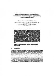
Left: segmented cell bodies (green), lobulated cell nuclei (yellow and red) and background (black), Middle: segmented cell nucleus extending outside border of host cell (red pixels), Right: the result of applying a morphological erosion operator; here the original partially overlaps relation changes to proper part . . . . . . A conceptual neighbourhood graph of RCC-8 . . . . . . . . . . . . . . . . . . . . Example of a spatio-temporal sequence based on RCC-8 . . . . . . . . . . . . . . Transition graph of the spatio-temporal sequence in Figure 4.3 . . . . . . . . . . An example UPQCN U of RCC-8 . . . . . . . . . . . . . . . . . . . . . . . . . . . The motif of the UPQCN U of RCC-8 shown in Figure 4.5 . . . . . . . . . . . . . Solution of the UPQCN U of RCC-8 shown in Figure 4.5 (i>2) . . . . . . . . . . .

2.7

4.2 4.3 4.4 4.5 4.6 4.7 5.1 5.2 5.3 5.4 5.5 5.6 5.7

16 19 22

70 71 72 73 80 81 82

Example of a chordal graph . . . . . . . . . . . . . . . . . . . . . . . . . . . . . . 89 Triangulation of the underlying constraint graph of a QCN . . . . . . . . . . . . . 91 Pruning capacity of -consistency restricted to a triangulation of the constraint graph of a QCN (partial -consistency) and standard -consistency on that QCN 92 Pruning capacity of -consistency (PC) over partial -consistency (PPC) . . . . . 93 A non-complete chordal graph G . . . . . . . . . . . . . . . . . . . . . . . . . . . 94 The ] operation on two QCNs accompanied by their respective graphs . . . . . . 99 QCNs with respect to their constraint graphs . . . . . . . . . . . . . . . . . . . . 102 xi

List of Figures 5.8 5.9 5.10 5.11 5.12 5.13 5.14 5.15 5.16 5.17 5.18 5.19 5.20 5.21 5.22 5.23 5.24 6.1 6.2

6.3 6.4

6.5 6.6 6.7 6.8 6.9

xii

Structures of a random regular graph with an average degree k = 9 and a scale-free graph with a preferential attachment m = 2, both having 100 nodes . . . . . . . Performance comparison of iPWC and PWC for RCC-8 networks . . . . . . . . . . Hash table based adjacency list for representing a chordal RCC-8 network . . . . Performance comparison for random scale-free RCC-8 networks . . . . . . . . . . Evidence of the power law node degree distribution of the real datasets considered Matrix representations of different graph configurations of adm1 . . . . . . . . . Experiment with random regular networks . . . . . . . . . . . . . . . . . . . . . Experiment with random scale-free-like networks . . . . . . . . . . . . . . . . . . Experiment with hard random scale-free-like networks . . . . . . . . . . . . . . . Experiment with hard random scale-free-like networks and a SAT implementation CPU time for series S(n, d, 6.5) of IA . . . . . . . . . . . . . . . . . . . . . . . . . CPU time for instances of RCC-8 not forced to be consistent . . . . . . . . . . . A graph and its partitioning graph with the parts comprising it (also contained in dashed circles in the initial graph) . . . . . . . . . . . . . . . . . . . . . . . . . A graph and its partitioning graph with the parts comprising it (also contained in dashed circles in the initial graph) . . . . . . . . . . . . . . . . . . . . . . . . . A chordal graph and its partitioning graph with the parts comprising it (also contained in dashed circles in the initial graph) . . . . . . . . . . . . . . . . . . . A graph G (top) with its biconnected components (middle) and its tree decomposition (bottom) . . . . . . . . . . . . . . . . . . . . . . . . . . . . . . . . . . . . . A separable constraint graph with an articulation vertex v . . . . . . . . . . . . . A countably infinite sequence of satisfiable atomic QCNs that agree on their common part . . . . . . . . . . . . . . . . . . . . . . . . . . . . . . . . . . . . . . . . A countably infinite sequence of satisfiable atomic QCNs that contains a subsequence which begins and ends with two QCNs representing the same set of spatial constraints (i.e., a sub-sequence which defines a loop between two QCNs) (a); we can reduce the sub-sequence to just considering the first QCN and patch it with the QCN following the sub-sequence (b) . . . . . . . . . . . . . . . . . . . . . . . A LUPQCN formula φ over timeline t . . . . . . . . . . . . . . . . . . . . . . . . . A countably infinite sequence of not trivially inconsistent and -consistent QCNs, where there exists a point of time t after which the QCNs in the sequence represent the same set of constraints . . . . . . . . . . . . . . . . . . . . . . . . . . . . . . . A L1 formula and its simplified tableau . . . . . . . . . . . . . . . . . . . . . . . The example spatio-temporal sequence and its corresponding transition graph of Section 4.3 . . . . . . . . . . . . . . . . . . . . . . . . . . . . . . . . . . . . . . . . A conceptual neighbourhood graph . . . . . . . . . . . . . . . . . . . . . . . . . . Example of the construction of a transition graph through algorithm Arachni . . . Example of a QSCN of Rectangle Algebra . . . . . . . . . . . . . . . . . . . . . .

106 108 121 125 127 127 128 130 131 132 141 142 148 149 151 152 157

163

164 166

167 175 179 181 184 191

Chapter 1

Introduction Qualitative Spatial and Temporal Reasoning (QSTR) is a major field of study in Artificial Intelligence and, particularly, in Knowledge Representation, which deals with the fundamental cognitive concepts of space and time in an abstract manner. This qualitative manner of dealing with space and time is in line with the qualitative abstractions of spatial and temporal aspects of the common-sense background knowledge on which the human perspective of physical reality is based. For instance, in natural language we use verbs such as inside, before, and north of to spatially or temporally relate one object with another object or oneself, without resorting to providing quantitative information about these entities. More formally, qualitative spatial and temporal reasoning restricts the rich mathematical theories that deal with spatial and temporal entities to simple qualitative constraint languages. The conciseness of the constraint languages used in the qualitative approach provides a promising framework that further boosts research and applications in spatial and temporal reasoning, as it allows for rather inexpensive reasoning about entities located in space and time. For example, some of these calculi may be implemented for handling spatial Geographic Information Systems (GIS) queries efficiently and some may be used for navigating and communicating with a mobile robot [Hazarika, 2012; Bhatt et al., 2011]. The first constraint language to deal with space or time in a qualitative manner was proposed by Allen in [Allen, 1981; Allen, 1983], called Interval Algebra, and it has been mostly used for reasoning about time ever since. Allen wanted to define a framework for reasoning about time in the context of natural language processing that would be reliable and efficient enough for reasoning about extracted and newly indrocuded temporal information in a qualitative manner. In particular, Interval Algebra uses intervals on the timeline to represent entities corresponding to actions, events, or tasks. Interval Algebra has become one of the most well-known qualitative constraint languages, due to its use for representing and reasoning about temporal information in various applications. Specifically, typical applications of Interval Algebra involve planning and scheduling [Allen and Koomen, 1983; Allen, 1991; Pelavin and Allen, 1987; Dorn, 1995], natural language processing [Song and Cohen, 1988], temporal databases [Snodgrass, 1987; Chen and Zaniolo, 1998], multimedia databases [Little and Ghafoor, 1993], molecular biology [Golumbic and Shamir, 1993] (e.g., arrangement of DNA segments/intervals along a linear chain involves particular temporal-like problems [Benzer, 1959]), and workflow [Lu et al., 2006]. Inspired by the success of Interval Algebra, Randell, Cui, and Cohn developed the Region Connection Calculus (RCC) in [Randell et al., 1992]. As its name suggests, the Region Connection Calculus studies the different relations that can be defined between regions in some topological space; these relations are based on the primitive relation of connection. As an example of a 1

Chapter 1. Introduction relation of the Region Connection Calculus, the relation disconnected between two regions x and y suggests that none of the points of region x connects with a point of region y, and vice versa. Two of its fragments, namely, RCC-8 and RCC-5 (a sublanguage of RCC-8 where no significance is attached to boundaries of regions), have been used in several real-life applications. In particular, Bouzy in [Bouzy, 2001] used the RCC-8 qualitative constraint language in programming the Go game, and Andreas et al. in [Lattner et al., 2005] used RCC-5 to set up assistance systems in intelligent vehicles. Other typical applications of the Region Connection Calculus involve GIS, robot navigation, high level vision, and natural language processing [Bhatt et al., 2011]. In the literature, there have also been efforts towards combining space and time in an interrelated manner and, consequently, forming spatio-temporal formalisms. With such qualitative spatio-temporal frameworks, we can represent for example the fact that a given region was contained in another region at one point in time and externally connected to that region at a next point of time, or even the fact that a point will always move towards a particular direction over time. Towards constraint-based qualitative spatio-temporal reasoning, most of the work has relied on formalisms based on the propositional temporal logic (PTL), also known as linear temporal logic, and some qualitative spatial constraint language, like the RCC-8 language we referenced earlier (cf. [Wolter and Zakharyaschev, 2003; Wolter and Zakharyaschev, 2000b]). PTL [Huth and Ryan, 2004] is the well known temporal logic comprising operators U (until), # (next point in time), 2 (always), and 3 (eventually) over various flows in time, such as hN, 0 16

2.1 Line Conditions.

2.3. Cases of Qualitative Spatial and Temporal Constraint Languages boundary (∂), and exterior (−) of regions A and B. The maximum number of dimensions of the intersection is 0 for points, 1 for lines, and 2 for areas. The interested reader may find more information about possible relations between areas, lines and points, and their respective calculi that can be defined in the dimensionally extended 9-intersection model in [Clementini et al., 1993].

2.3.7

Orientation Calculi

Orientation relations describe the orientation between two spatial entities with respect to a third object. As such, a binary relation between a primary spatial entity and a reference spatial entity is, in general, not sufficient to describe the orientation between those entities, since some kind of frame of reference must also be considered [Cohn, 1997]; after doing so, one is then able to define an explicit ternary relation upon the primary spatial entity, the reference spatial entity, and the frame of reference. Many orientation constraint languages are defined using this approach [Freksa, 1992; Isli and Cohn, 2000; Schlieder, 1993; Röhrig, 1994], while others presuppose an immutable extrinsic frame of reference (e.g., gravitation, a fixed coordinate system) as in the calculus of dinstances and cardinal directions presented in [Frank, 1992] (also cf. [Hernández, 1994]) or a natural intrinsic orientation that is exhbitited by certain spatial entities (e.g., humans, buildings) as in the OPRAm calculus presented in [Moratz et al., 2005; Mossakowski and Moratz, 2012; Moratz, 2006]. Regarding orientation constraint languages based on explicit ternary relations, of particular interest is the approach of Schlieder where triples of points are mapped to one of the three qualitative values +, 0, and −, denoting anticlockwise, colinear, and clockwise orientations respectively [Schlieder, 1993]. The approach of Schlieder can be used for reasoning about visible locations in qualitative navigation tasks [Schlieder, 1993], for shape description [Schlieder, 1996], or to develop a qualitative constraint language for reasoning about the relative orientation of pairs of line segments [Schlieder, 1995]. Another important ternary orientation constraint language is that of Röhrig [Röhrig, 1994; Röhrig, 1993] which is based on the ternary relation CY CORD(x, y, z) that is true in the 2-dimensional space when x, y, and z are in clockwise orientation. Röhrig also demonstrates how some qualitative constraint languages can be interpreted using the CY CORD(x, y, z) relation and, thus, exploit his reasoning system that builds on that relation [Röhrig, 1993]. Regarding orientation constraint languages based on an extrinsic frame of reference, it is most common to use some global reference direction, which allows the orientation between two objects to be represented with respect to the reference direction using just binary relations (e.g., compass directions as in [Frank, 1992]). Such approaches were later generalised to form the Star algebra [Renz and Mitra, 2004; Mitra, 2004; Mitra, 2002]. Regarding orientation constraint languages based on a natural intrinsic orientation, the OPRAm calculus [Moratz et al., 2005; Mossakowski and Moratz, 2012; Moratz, 2006] is among the most seasoned qualitative constraint languages for reasoning about qualitative relative direction information. In OPRAm , oriented points, i.e., pairs of a point and a direction on the 2-dimensional plane, serve as the basic entities since they are the simplest spatial entities that have an intrinsic orientation. Sets of base relations can have adjustable granularity levels in this calculus. Further, OPRAm offers simple geometric rules for computing the calculus’s compositions based on triples of oriented points. 17

Chapter 2. Qualitative Spatial and Temporal Constraint Languages

2.4

Relational Operations

Given a set of base relations B of a qualitative constraint language, we have that B is closed under the converse operation (−1 ). In particular, the converse operation associates a relation r−1 ∈ 2B with each base relation b ∈ B, which is defined by r−1 = {b0 ∈ B | ∃x, y ∈ D with x b y and y b0 x}. The converse operation can be generalized to total set of relations 2B as follows. For each S the −1 B −1 −1 relation r ∈ 2 , r is defined by r = b∈r b . For every x, y ∈ D and r ∈ 2B , it also −1 holds that y r x if x r y. The inverse is not necessarily true in the general case [Dylla et al., 2013]. For most of the qualitative constraint languages, there exists for each base relation b ∈ B a single base relation of B that corresponds to the converse of b, viz., the relation {(y, x) | (x, y) ∈ b}. For these languages, the converse relation of any base relation b ∈ B is b−1 , which is a base relation of B. Moreover, for every x, y ∈ D and r ∈ 2B we have that x r y if and only if y r−1 x. Examples of qualitative constraint languages for which the converse of a base relation corresponds to a relation comprising more than one base relations are the Cardinal Direction (Relations) Calculus (CDR) [Skiadopoulos and Koubarakis, 2005] and its recently introduced rectangular variant (RDR) [Navarrete et al., 2013]. The converse of a relation 2B can be obtained from a converse table which stores the converse base relation b−1 for each base relation b ∈ B. The converse tables of some of the most well-known qualitative constraints languages that we presented earlier are given in Table 2.2. Given for example the RCC-8 relation {DC, T P P i, N T P P } we can easily derive its converse relation, viz., relation {DC, T P P, N T P P i}, thus, {DC, T P P i, N T P P }−1 = {DC, T P P, N T P P i}. Appart from the converse operation (−1 ), 2B is also equipped with the usual set-theoretic operations, viz., union and intersection, and the weak composition operation denoted by symbol  [Renz and Ligozat, 2005]. Given two relations r, r0 ∈ 2B , r ∪ r0 corresponds to a relation of 2B that comprises the base relations of B that exist in either r or r0 . In a similar manner, r ∩ r0 corresponds to a relation of 2B that comprises the base relations of B that exist in both r and r0 . The weak composition operation is a bit more complex to define than the relational operations we discussed so far. Let us first recall the relational composition which is defined by b ◦ b0 ={(x, y)|∃z : (x, z) ∈ b ∧ (z, y) ∈ b0 } for two base relations b, b0 ∈ B. According to the definition of relational composition, we have to look at an infinite number of tuples in order to Table 2.2: Converse tables for (a) Point Algebra, (b) Cardinal Direction Calculus, (c) Interval Algebra, and (d) RCC-8 (a)

18

(b)

(c)

(d)

b

b−1

b

b−1

b

b−1

b

b−1

< > =

> < =

N NW W SW S SE E NE EQ

S SE E NE N NW W SW EQ

b bi o oi m mi d di si s f fi eq

bi b oi o mi m di d s si fi f eq

DC EC PO TPP TPPi NT P P NT P P i EQ

DC EC PO TPPi TPP NT P P i NT P P EQ

2.4. Relational Operations

z y x

z y

z

x y

x N T P P (x, z)

T P P (x, z)

P O(x, z)

Figure 2.7: Three possible configurations for regions x, y, z when we have EC(x, y) and N T P P (y, z)

compute the composition of base relations, which is clearly not feasible. Fortunately, many domains such as points or intervals in a timeline are ordered or, otherwise, well-structured domains and composition can be computed using the semantics of the relations. However, for domains such as arbitrary spatial regions that are more vague and where there is no common representation for the entities we consider, computing the true composition is not feasible and composition has to be approximated by using a weaker variant of it, called weak composition [Renz and Ligozat, 2005]. Formally, the weak composition () of two base relations b, b0 ∈ B is defined as the strongest relation r ∈ 2B which contains b ◦ b0 , or formally, b  b0 ={b00 ∈ B|b00 ∩(b ◦ b0 ) 6= ∅}. The advantage of weak composition is that we stay within the given set of relations 2B while applying the algebraic operations, as 2B is by definition closed under weak composition, union, intersection, and converse. As an example, let us consider the RCC-8 base relations of EC and N T P P . The weak composition EC  N T P P yields the set of base relations {N T P P , T P P , P O}, as shown in Figure 2.7. The obtained set corresponds to all the base relations that can be possible between regions x and z when we have that EC(x, y) and N T P P (y, z). Let us now also see why RCC-8, for instance, has only weak composition and not relational composition. Consider the RCC-8 set of constraints {T P P (x, y), EC(x, z), T P P (z, y)}. It can be verified that T P P ∈ EC  T P P , EC ∈ T P P  T P P −1 , and T P P ∈ EC −1  T P P . As such, assuming that relational composition holds, we should be able to extract a valid configuration using and starting with any of the infinite available tuples that satisfy relation T P P or EC. However, if we pick a tuple (x, y) for satisfying relation T P P such that y is instantiated as a region with two disconnected pieces and x completely fills one piece, then z cannot be instiantiated. So, T P P 6∈ EC ◦ T P P and, consequently, relational composition does not hold for RCC-8. As noted earlier, well-structured domains such as points or intervals in a timeline are ordered and composition can be computed using the semantics of the relations. For example, for Point Algebra and Interval Algebra, with their usual domains based on Q as presented earlier, weak composition is equivalent to relational composition, i.e., we have that r  r0 = r ◦ r0 for every r, r0 ∈ 2B . For qualitative constraint languages for which relational composition does not hold, we have that r ◦ r0 ⊂ r  r0 for some r, r0 ∈ 2B , as we also demonstrated in the case of RCC-8. A complete analysis on the relations of RCC-8 for which relational composition does not hold is provided in [Li and Wang, 2006]. The weak composition operation can be generalized to the S total set of relations 2B as follows. For every r, r0 ∈ 2B , we have that r  r0 = b∈r,b0 ∈r0 b  b0 . The weak composition of two relations r, r0 ∈ 2B can be facilitated by a weak composition table which stores the weak compositions among all base relations of the considered qualitative constraint language. The weak composition tables of Point Algebra and RCC-8 are given in Table 2.3. Given for example the RCC-8 relations {T P P, N T P P } and {T P P } we can easily 19

Chapter 2. Qualitative Spatial and Temporal Constraint Languages Table 2.3: Weak composition tables for (a) Point Algebra and (b) RCC-8 (a) 




=

< > =

< B
>

< > =

(b) 

DC

EC

PO

TPP

NTPP

TPPi

NTPPi

EQ

DC

B

DC, EC, P O, TPP, NT P P EC, P O, TPP, NT P P

DC, EC, P O, TPP, NT P P P O, TPP, NT P P

DC

DC

DC, EC, P O, T P P i, NT P P i

DC, EC, P O, TPP, NT P P DC, EC, P O, TPP, NT P P

DC

EC

DC, EC

DC

EC

PO

B

P O, TPP, NT P P

P O, TPP, NT P P

DC, EC, P O, TPP, NT P P

TPP, NT P P

NT P P

DC, EC, P O, T P P i, NT P P i DC, EC, P O, T P P i, NT P P i

NTPP

DC

DC

NT P P

NT P P

TPPi

DC, EC, P O, T P P i, NT P P i DC, EC, P O, T P P i, NT P P i

EC, P O, T P P i, NT P P i

DC, EC, P O, TPP, NT P P P O, T P P i, NT P P i

P O, TPP, NT P P

P O, T P P i, NT P P i

P O, T P P i, NT P P i

P O, TPP, T P P i, EQ P O, T P P i, NT P P i

DC, EC, P O, T P P i, NT P P i DC, EC, P O, TPP, T P P i, EQ DC, EC, P O, TPP, NT P P T P P i, NT P P i

PO

TPP

DC, EC, P O, T P P i, NT P P i DC

DC, EC, P O, TPP, NT P P DC, EC, P O, TPP, T P P i, EQ DC, EC, P O, T P P i, NT P P i DC, EC

DC

EC

PO

TPP

NTPPi

EQ

P O, TPP, NT P P , T P P i, N T P P i, EQ NT P P

TPP

B

NT P P

NT P P i

TPPi

NT P P i

NT P P i

NT P P i

TPPi

NT P P i

EQ

derive relation {T P P, N T P P } by performing the following operation: {T P P, N T P P }  {T P P } = (T P P  T P P ) ∪ (N T P P  T P P ) = {T P P, N T P P } ∪ {N T P P } = {T P P, N T P P }. The weak composition operation  along with the converse operation −1 , and the total set of relations 2B along with the identity relation Id of a qualitative constraint language (where B is its set of base relations), form an algebraic structure (2B , Id, ,−1 ) which can correspond to a relation algebra for some qualitative constraint languages in the sense of Tarski [Tarski, 1941; Dylla et al., 2013]. This topic has been extensively discussed in [Ligozat and Renz, 2004; Dylla et al., 2013]. In [Dylla et al., 2013] the authors thoroughly analyze existing qualitative constraint languages and provide a classification involving different notions of relation algebra. In fact, we 20

2.5. Classes of Relations Table 2.4: Axioms for relation algebras, where r, s, t ∈ 2B Axiom ∪-commutativity ∪-associativity Huntington axiom -associativity -distributivity identity law −1 -involution −1 -distributivity −1 -involutive distributivity Tarski/de Morgan axiom

Definition r∪s=s∪r r ∪ (s ∪ t) = (r ∪ s) ∪ t r∪s∪r∪s=r r  (s  t) = (r  s)  t (r ∪ s)  t = (r  t) ∪ (s  t) r  Id = r (r−1 )−1 = r (r ∪ s)−1 = r−1 ∪ s−1 (r  s)−1 = s−1  r−1 r−1  r  s ∪ s = s

have the following result: Proposition 1 (cf. [Dylla et al., 2013]) Each of the qualitative constraint languages of Point Algebra, Cardinal Direction Calculus, Interval Algebra, Block Algebra, and RCC-8 is a relation algebra with the algebraic structure (2B , Id, ,−1 ). In what follows, for a qualitative constraint language that is a relation algebra with the algebraic structure (2B , Id, ,−1 ), we will simply say that it is a relation algebra as the algebraic structure will always be of the same format. In our context, a relation algebra is nothing more than a qualitative constraint language that satisfies certain axioms. These axioms are listed in Table 2.4 and allow for several optimizations when designing algorithms for reasoning with qualitative constraint languages. For instance, -associativity ensures that if we need to compute r  s  t for some relations r, s, t ∈ 2B , we can do so by choosing to compute either r  (s  t) or (r  s)  t, i.e., we do not need to compute the operation both from left to right and from right to left. Due to the fact that the most interesting and well-known spatial and temporal calculi are relation algebras (cf. Proposition 1), and for the sake of simplicity in the presentation of our algorithms in what follows in the thesis, we will focus on qualitative constraint languages that are relations algebras and, hence, satisfy the related axioms.

2.5

Classes of Relations

As mentioned earlier, 2B is by definition closed under weak composition, union, intersection, and converse. In the context of the algorithms that are studied in this thesis, we deal with particular subsets of relations of 2B that are closed under threee of the four aforementions relational operations, namely, weak composition, intersection, and converse. We call such subsets of relations subclasses of relations. Clearly, the entire set of relations 2B is a class of relations by itself. Formally, we define a subclass of relations as follows. Definition 1 A subclass of relations is a subset A ⊆ 2B that contains the singleton relations of 2B and B and is closed under converse, intersection, and weak composition. Given a relation r of 2B and a subclass A ⊆ 2B , A(r) will denote the smallest (with respect to the number of base relations) relation of A including r. 21

Chapter 2. Qualitative Spatial and Temporal Constraint Languages pi mi oi f

si eq di

d s

fi o

m p

Figure 2.8: The lattice of Interval Algebra

2.5.1

Distributive Subclasses of Relations

The notion of distributive subclasses of relations will be important in what follows in the thesis, hence, we accomodate a separate section here to properly define it. Given three relations r, r0 , and r00 , we say that weak composition distributes over intersection if we have that r  (r0 ∩ r00 ) = (r  r0 ) ∩ (r  r00 ) and (r0 ∩ r00 )  r = (r0  r) ∩ (r00  r). Definition 2 A subclass A ⊆ 2B is a distributive subclass if weak composition distributes over non-empty intersections for all relations r, r0 , r00 ∈ A. A subclass A ⊆ 2B is a maximal distributive subclass if there exists no other distributive subclass that properly contains A. The distributivity of a class of relations is a new concept introduced in [Duckham et al., 2014; Li et al., 2015a] and thoroughly analysed in [Long and Li, 2015]. However, there exist several examples in the literature where the authors implicitly or explicitly exploited the fact that for certain subclasses of relations for a considered qualitative constraint language weak composition distributes over non-empty intersection for all relations of that subclass. As an example, van Beek and Cohen observed this property for the subclass of convex relations of Point Algebra [van Beek and Cohen, 1990]. (This observation also exists in the PhD Thesis of van Beek [Van Beek, 1990].) In another example of this property, Chandra and Pujari implicitly consider the distributivity of a subclass of convex relations for RCC-8 in their proof of Theorem 8 in [Chandra and Pujari, 2005] that involves a special reasoning problem of RCC-8 networks, viz., the minimal labeling problem, which we have already mentioned and briefly explained earlier on in the introductory chapter of the thesis and will formally define later on in Section 3.3. More recently, Amaneddine and Condotta in [Amaneddine and Condotta, 2012] identified maximal distributive subclasses of relations for Point Algebra and Interval Algebra in their effort to guarantee a particular strong characterization for networks of the aforementioned qualitative constraint languages through a polynomial algorithm. What is more interesting, is the fact that all subclasses of convex relations that have been defined in the literature for the most well-known qualitative constraint languages, 22

2.6. Conclusion viz., Point Algebra, Interval Algebra, Cardinal Direction Calculus, Block Algebra, and RCC-8, turn out to be maximal distributive sublasses of relations for these languages [Long and Li, 2015]. This is due to the fact that subclasses of convex relations and distributive subclasses of relations share a very important common property, viz., they exhibit convexity in Helly’s sense [Danzer et al., 1963]. As such, distributive subclasses of relations generalize the notion of subclasses of convex relations. However, for the sake of completeness, let us introduce the notion of convexity for relations of qualitative constraint languages and its relationship with distributive subclasses of relations. In general, to define a subclass of convex relations for a given qualitative constraint language, one has to take into account the semantics of the base relations of the set B of that language and assume a geometrical characterization of the language as well, and first obtain a partial ordering [Dushnik and Miller, 1941] on its set of base relations (B, ). Such a partially ordered set is most often represented by a Hasse diagram [Birkhoff, 1948]. As an example, Ligozat in [Ligozat, 1994] defines a partially ordered set (B, ) for Interval Algebra, which is represented by the Hasse diagram shown in Figure 2.8 (referred to as a lattice due to the form of the Hasse diagram depicting it). The interpretation of the lattice of Interval Algebra with respect to convexity is as follows. For b1 , b2 ∈ B with b1  b2 , we write [b1 , b2 ] as the set of base relations b such that b1  b  b2 , and call such a relation a convex relation. Hence, the total set of convex relations can be obtained by enumerating the intervals in the lattice. For example, relation {d, s, o, m} in Interval Algebra is convex as it correponds to interval [d, m] in the lattice. As we will stick with distributive subclasses of relations in the context of this thesis, we will not delve more into the details of convexity and convex relations. The interested reader is kindly asked to refer to [Ligozat, 2011] for a complete analysis of the aforementioned notions. An observation is that subclasses of convex relations for Point Algebra, Interval Algebra, Cardinal Direction Calculus, Block Algebra, and RCC-8 are Helly [Long and Li, 2015]. A Helly subclass of relations is defined as follows. Definition 3 A subclass A ⊆ 2B is Helly if and only if for any n relations r1 , r2 , . . . rn ∈ A we have: n \ ri 6= ∅ iff (∀1 ≤ i, j ≤ n) ri ∩ rj 6= ∅ i=1

Then, we have the following result by Long and Li in [Long and Li, 2015]: Theorem 1 ([Long and Li, 2015]) A subclass A ⊆ 2B for a qualitative constraint language that is a relation algebra is distributive if and only if it is Helly. Maximal distributive subclasses of qualitative spatial and temporal constraint languages can be identified through an automatic procedure as described in [Long and Li, 2015]. In the simplest case, identifying a maximal distributive subclass for some qualitative constrtaint language can ˆ\ be done with a brute-force procedure that checks if B ∪ Z satisfies distributivity for some subset B ˆ Z ⊂ 2 , where X denotes the closure under converse, intersection, and weak composition for a subset X ⊆ 2B .

2.6

Conclusion

In this chapter, we introduced various qualitative constraint-based formalisms for reasoning about time and space. More precisely, we introduced the algebraic structure upon which such formalisms are defined, which comprises a set of base relations and certain standard relational 23

Chapter 2. Qualitative Spatial and Temporal Constraint Languages operations. In particular, the set of base relations of a given qualitative constraint language allows us to represent the definite knowledge between any two or more entities with respect to the given level of granularity. Moreover, the indefinite knowledge between any two or more entities can be represented by unions of possible base relations. Regarding relational operations, we defined the converse operation and the weak composition operation, both of which are essential in being able to reason with the relations of a qualitative constraint language. For instance, given two entities and the knowledge of how the first entity is related to the second one, the converse operation allows us to obtain the knowledge of how the second entity is related to the first one. The weak composition operation allows us to eliminate certain configurations among entities for which we already have some partial knowledge. As an example, if we know that a temporal event occurs before a second temporal event, which in turn occurs before a third temporal event, the weak composition operation allows us to infer that the first temporal event occurs befores the third temporal event. We used various representative examples to highlight the different types of relations that are considered by a spatial or temporal qualitative constraint language. As a matter of fact, we considered qualitative constraint languages based on points, intervals, blocks, and even regions, and we also focused on some aspects of orientation and the means by which it can be handled. Of course, the list of qualitative constraint languages that we presented is far from exhaustive, but it is sufficient for motivating our contributions that we will present later on.

24

Chapter 3

Reasoning with Qualitative Constraint Networks 3.1

Introduction

In this chapter, we formally introduce the notion of a qualitative constraint network (QCN), and draw the connection between the relational operations presented in the previous chapter and some useful local consistency conditions for characterizing QCNs. We present the fundamental reasoning problems associated with QCNs, overview the state of the art algorithms for dealing with those problems, and explain some constraint properties of QCNs. Finally, we discuss about some decomposability aspects of QCNs considered in the literature. A QCN comprises a set of variables corresponding to a set of spatial or temporal entities and a set of relations that constrain the possible qualitative configurations between the different entities. Given a QCN over a set of variables corresponding to a set of spatial or temporal entities, we are particularly interested in its satisfiability problem, that is, deciding whether there exists an interpretation of all the variables of the QCN such that all of its constraints are satisfied by this interpretation; such an interpretation being called a solution. The satisfiability problem is closely related to the minimal labeling problem and the redundancy problem, in the sense that the latter two problems exhibit functions that build on the core algorithms used to obtain a solution of a QCN. In particular, the minimal labeling problem is the problem of determining all the base relations for each of the constraints of a QCN that participate in at least one of its solutions, whilst the redundancy problem is the problem of obtaining all the non-redundant constraints of a QCN, i.e., those constraints that do not contain at least one base relation participating in a solution of the modified QCN that results by removing these constraints. Depending on the subset of relations of a qualitative constraint language over which a given QCN is defined, certain characterizations of that QCN can be established that allow us to deal with the aforementioned reasoning problems in polynomial time; this is typically achieved through the use of specialized local consistency conditions and related algorithms. Moreover, and always in relation to the discussed reasoning problems, we will see how certain constraint properties in the context of qualitative constraint-based reasoning allow us to exploit the structure of some special cases of QCNs and deal with them in a more efficient manner. 25

Chapter 3. Reasoning with Qualitative Constraint Networks

3.2

Qualitative Constraint Networks (QCNs)

As we already discussed, qualitative constraint languages use relations to encode spatial or temporal knowledge between entities. Hence, it comes natural to use constraints to capture these relations. In what follows, sometimes we will refer to constraints as relations when it is clear from the context that a particular relation along with some entities forms a constraint upon those entities. The problem of reasoning about qualitative spatial or temporal information can be modelled as an infinite-domain variant of a Constraint Satisfaction Problem (CSP) [Montanari, 1974], for which we use the term Qualitative Constraint Network (QCN). For instance, there are infinitely many time points or temporal intervals in the timeline and infinitely many regions in a two or three dimensional space. Formally, a QCN is defined as follows. Definition 4 A qualitative constraint network (QCN) is a pair (V, C) where: • V = {v1 , . . . , vn } is a non-empty finite set of variables each of which corresponds to a set of spatial or temporal entities; • C is a mapping that associates a relation r ∈ 2B with each pair (v, v 0 ) of V × V , that relation being denoted by C(v, v 0 ). Mapping C is such that C(v, v) = {Id} and C(v, v 0 ) = (C(v 0 , v))−1 for every v, v 0 ∈ V . An example of a QCN of RCC-8 is shown in Figure 3.1 along with a corresponding spatial configuration. In particular, the QCN comprises the set of variables {x, y, z} and the constraints C(x, y) = C(y, z) = C(z, x) = {EC}. Converse relations as well as Id loops are not mentioned or shown in the figure for simplicity. Note that we always regard a QCN as a complete network. In what follows, given a QCN N = (V, C) and v, v 0 ∈ V , relation C(v, v 0 ) will also be denoted by N [v, v 0 ]. We have the following definitions regarding QCNs: Definition 5 Let N = (V, C) be a QCN, then: • a partial solution of N on V 0 ⊆ V is a valuation σ of the variables of V 0 such that for each pair of variables (u, v) ∈ V 0 × V 0 , we have that σ(u) and σ(v) satisfy C(u, v), i.e., there exists a base relation b ∈ C(u, v) such that (σ(u), σ(v)) ∈ b; • a solution of N is a partial solution on V ; • a QCN N 0 is equivalent to N if and only if it admits the same set of solutions with N ; • a sub-QCN1 N 0 of N , denoted by N 0 ⊆ N , is a QCN (V 0 , C 0 ) such that V 0 = V and C 0 (v, v 0 ) ⊆ C(v, v 0 ) ∀v, v 0 ∈ V ; • N is atomic if it comprises only singleton relations, where a singleton relation is a relation {b} for some base relation b ∈ B; • a scenario S of N is an atomic satisfiable sub-QCN of N ; • a partial scenario of N on V 0 ⊆ V is a scenario restricted to constraints involving only variables of V 0 ; 1

26

This term is also found by the name “refined QCN” throughout the literature.

3.2. Qualitative Constraint Networks (QCNs)

x {EC}

z

y

{EC}

x

y

z

{EC}

Figure 3.1: A QCN of RCC-8 along with its spatial configuration (note that region y has a hole) • a base relation b ∈ C(v, v 0 ), with v, v 0 ∈ V , is feasible (resp. unfeasible) iff there exists (resp. there does not exist) a scenario S = (V, C 0 ) of N such that C 0 (v, v 0 ) = {b}; • the constraint graph of N is the graph (V, E), denoted by G(N ), for which we have that {v, v 0 } ∈ E iff C(v, v 0 ) 6= B;2 • N is said to be trivially inconsistent iff ∃v, v 0 ∈ V with C(v, v 0 ) = ∅; • ⊥V will denote the QCN N whose each constraint between each pair of variables (v, v 0 ) ∈ V × V is defined by the empty relation ∅. Let us further introduce some operations with respect to QCNs. Given a QCN N = (V, C) and v, v 0 ∈ V , we have that: • N[v,v0 ]/r with r ∈ 2B yields the QCN N 0 = (V, C 0 ) defined by C 0 (v, v 0 ) = r, C 0 (v 0 , v) = r−1 and C 0 (y, w) = C(y, w) ∀(y, w) ∈ (V × V ) \ {(v, v 0 ), (v 0 , v)}; • N ↓V 0 , with V 0 ⊆ V , yields the QCN N restricted to V 0 . Given two QCNs N = (V, C) and N 0 = (V, C 0 ) of the same set of variables V , we have that: • N +N 0 yields the QCN N 00 = (V, C 00 ), where C 00 (v, v 0 ) = C(v, v 0 )∪C 0 (v, v 0 ) for all v, v 0 ∈ V . Given two QCNs N = (V, C) and N 0 = (V 0 , C 0 ) such that C(u, v) = C 0 (u, v) for every u, v ∈ V ∩ V 0 , we have that: • N ∪ N 0 yields the QCN N 00 = (V 00 , C 00 ), where V 00 = V ∪ V 0 , C 00 (u, v) = C 00 (v, u) = B for all (u, v) ∈ (V \ V 0 ) × (V 0 \ V ), C 00 (u, v) = C(u, v) for every u, v ∈ V , and C 00 (u, v) = C 0 (u, v) for every u, v ∈ V 0 . Finally, given a QCN N = (V, C) and a subclass A ⊆ 2B , we have that: • A(N ) yields the QCN N 0 = (V, C 0 ) defined by C 0 (v, v 0 ) = A(C(v, v 0 )) ∀v, v 0 ∈ V . The aforementioned binary operations on QCNs are presented in Figure 3.2 for clarity. 2

Note that the constraint graph of a QCN does not involve the universal relation B as it is the non-restrictive relation that contains all base relations, thus, it does not really pose a constraint. (The result of the weak composition of any relation with the universal relation is the universal relation.)

27

Chapter 3. Reasoning with Qualitative Constraint Networks

x

x {EC, P O}

{DC, EC}

{DC, P O, T P P } {DC, EC}

z

y

y

{P O, T P P }

N1

B {DC, EC}

{N T P P }

y

{N T P P }

N2

x

{DC, P O, T P P }

w

w

{EC, P O}

z

{P O, T P P }

N1 ∪ N 2 x

x {EC, P O, T P P }

{EC}

y

{DC, T P P } {DC}

z

y

{T P P, T P P I}

N3

z {N T P P I}

N4

x

{DC, EC, P O, T P P } {DC, EC}

z

y {T P P, T P P I, N T P P I} N3 + N4 Figure 3.2: Binary operations on QCNs

3.3

Reasoning Problems Associated with QCNs

Given a QCN, we are particularly interested in its satisfiability problem, that is, the problem of deciding whether there exists an interpretation of all the variables of the QCN such that all its constraints are satisfied by this interpretation; such an interpretation being called a solution as defined earlier. The satisfiability problem is closely related to the minimal labeling problem (MLP) [Montanari, 1974] (cf. [Liu and Li, 2012]) and the redundancy problem [Duckham et al., 2014; Li et al., 2015a], in the sense that the latter problems exhibit functions that build on the core algorithms used to obtain a solution of a QCN. We will view the aforementioned reasoning problems in detail in what follows. 28

3.3. Reasoning Problems Associated with QCNs

3.3.1

Satisfiability Problem

The satisfiability problem of QCN is among the most important problems associated with QCNs. We can formally define the satisfiability problem of a QCN as follows. Definition 6 The satisfiability problem, given a QCN N , is the problem of deciding whether N is satisfiable, i.e., whether it admits a solution. The satisfiability problem for most of the well-known qualitative constraint languages is NPcomplete. Specifically, and with the exception of Point Algebra, checking the satisfiability of an arbitrary QCN of RCC-8, Cardinal Direction Calculus, Interval Algebra, or Block Algebra is NPcomplete [Renz and Nebel, 1999; Ligozat, 1998; Nebel and Bürckert, 1995; Balbiani et al., 2002]. Checking the satisfiability of a QCN of Point Algebra can be done in polynomial time [van Beek, 1992]. In the literature, the usual approach for solving the satisfiability problem of a given QCN involves obtaining a scenario of that QCN. This is because we have a particular local consistency condition for deciding the satisfiability of atomic QCNs for many qualitative constraint languages, that we will discuss in a later section. Once the scenario is obtained, a solution of the QCN can be constructed in polynomial time using some canonical model, i.e., a structure that allows to model any satisfiable sentence of the qualitative constraint language. Of particular interest is the case of RCC-8, for which several canonical models have been defined in order to obtain interesting solutions, such as a domain of regular closed sets of the set of real numbers [Challita, 2012], a domain of countably many homeomorphic disjoint components of some topological space [Li and Wang, 2006; Li, 2006], and the usual domain of regions corresponding to regular closed subsets of some topological space that do not have to be internally connected and do not have a particular dimension [Renz, 2002a]. The canonical model of Renz, allows a simple representation of regions with respect to a set of RCC-8 constraints, and, further, enables one to generate realizations in any dimension d ≥ 1. As an example, let us view the QCN of RCC-8 in Figure 3.1. This QCN is atomic and also, clearly, satisfiable. As such, the QCN is also a scenario of itself. A solution σ of the QCN is shown to its left, where σ(x), σ(y), and σ(z) correspond to the 2-dimensional shapes tagged with x, y, and z respectively in the figure. As our domain is infinite, note that we can have an infinite number of solutions for any given scenario. There have been many works in the literature that try to solve the satisfiability problem of a non-tractable QCN3 in an efficient manner. All these works consider some kind of backtracking search (either iterative or recursive), a preprocessing operation to prune off certain unfeasible base relations that is based on a polynomial algorithm that makes use of weak composition, and, most importantly, a subclass of relations of 2B with the property that QCNs defined over that subclass become tractable [Nebel and Bürckert, 1995; Nebel, 1997; Renz and Nebel, 2001; Renz, 1999; Renz and Nebel, 1999; Balbiani et al., 2002; Balbiani et al., 1999; Ligozat, 1998]. Of course, for tractable QCNs, dedicated polynomial algorithms have been defined, as is the case for QCNs of Point Algebra where a polynomial method based on topological sort [Knuth, 1973] is defined in [van Beek, 1992, chap. 3]. We will review the approaches for solving the satisfiability problem of QCNs in more detail in the following sections, and we will also present our contributions for solving the satisfiability problem of QCNs later on in a separate chapter. 3

In what follows, as a convention, by saying that a QCN N is tractable (resp. non-tractable), we mean that the satisfiability problem for the class of QCNs that is defined by the restrictions imposed on N (if any) is tractable (resp. non-tractable), i.e., solvable (resp. not solvable) by a deterministic Turing machine in polynomial time.

29

Chapter 3. Reasoning with Qualitative Constraint Networks

v1 {EC, T P P }

v0

{N T P P i}

v2

{DC, P O}

v1 {EC}

v0

{N T P P i}

v2

{DC}

Figure 3.3: A RCC-8 network (left) and its minimal network (right)

3.3.2

Minimal Labeling Problem

The minimal labeling problem (MLP), also known as the deductive closure problem, is a fundamental problem in qualitative spatial and temporal reasoning which involves making all the constraints of a QCN minimal, i.e., obtaining the base relations participating in at least one solution for each of the constraints of that network. Definition 7 Given a QCN N = (V, C), we say that a relation C(v, v 0 ), with v, v 0 ∈ V , is minimal if and only if every base relation b ∈ C(v, v 0 ) is feasible. Notably, the MLP of a QCN is equivalent to the corresponding satisfiability problem with respect to polynomial Turing-reductions. As such, verifying if a QCN comprises only minimal relations is a NP-hard problem for QCNs for which the satisfiability problem is NP-complete (cf. [Liu and Li, 2012]). Since their introduction in 1974 [Montanari, 1974], minimal constraint networks have been the focus of study in both the constraint programming community (cf. [Gottlob, 2012]) and the qualitative spatial and temporal reasoning community [van Beek and Cohen, 1990; Gerevini and Saetti, 2011; Liu and Li, 2012; Chandra and Pujari, 2005; Amaneddine and Condotta, 2013; Bessière et al., 1996; Gerevini and Schubert, 1995; Amaneddine and Condotta, 2012]. We define the notion of a minimal QCN as follows. Definition 8 A QCN N = (V, C) is minimal if and only if ∀v, v 0 ∈ V we have that C(v, v 0 ) is minimal. Finally, the MLP of a QCN can be formally defined as follows. Definition 9 Given a QCN N , the minimal labeling problem (MLP) is the problem of obtaining the largest (with respect to ⊆) minimal sub-QCN N 0 of N . Solving the MLP of a given QCN involves prunning off unfeasible base relations iteratively until a state is reached where no more unfeasible base relations exist. In that state, all the constraints of the (possibly) modified QCN will be minimal and, thus, we will have obtained a minimal QCN. The unique equivalent minimal sub-QCN of a QCN N is denoted by Nmin . As an example, let us view the QCN N of RCC-8 in Figure 3.3 on the left hand. Network N is satisfiable, but not minimal, as it comprises unfeasible base relations. In particular, the base relation P O between variables v1 and v2 is unfeasible as P O 6∈ {N T P P i}−1  {EC, T P P } and, thus, it cannot participate in a solution. Likewise, base relation T P P (v0 , v1 ) is unfeasible as T P P 6∈ {N T P P i}  {DC, P O} and, thus, it also cannot participate in a solution. By removing the aforementioned two unfeasible base relations we obtain the minimal network on the right hand of the figure, i.e., network Nmin . In the literature, the works on obtaining the equivalent minimal sub-QCN of a QCN N have focused on identifying particular subclasses of relations of 2B for the qualitative constraint 30

3.3. Reasoning Problems Associated with QCNs language considered for which minimality can be guaranteed through a polynomial algorithm [van Beek and Cohen, 1990; Gerevini and Saetti, 2007; Gerevini and Saetti, 2011; Liu and Li, 2012; Chandra and Pujari, 2005; Amaneddine and Condotta, 2013; Bessière et al., 1996; Gerevini and Schubert, 1995; Amaneddine and Condotta, 2012]. In the particular case of [Amaneddine and Condotta, 2013], the authors go a step further by proposing a backtracking search algorithm that iteratively prunes off unfeasible base relations of a given QCN N until Nmin is obtained. We will review the approaches for solving the MLP of QCNs in more detail in the following sections, and we will also present our contributions for solving the MLP of QCNs later on in a separate chapter.

3.3.3

Redundancy Problem

Recently, the important problem of deriving redundancy in a RCC-8 network was considered and already well established in [Duckham et al., 2014; Li et al., 2015a]. For a RCC-8 network N a constraint is redundant, if removing that constraint from N (i.e., replacing that constraint with the universal relation) does not change the solution set of N . A prime network of N is a network which contains no redundant constraints, but has the same solution set as N . Finding a prime network can be useful in many applications such as computing, storing, and compressing the relationships between spatial objects and hence saving space for storage and communication, facilitating comparison between different networks, merging networks [Condotta et al., 2008; Condotta et al., 2009], aiding quering in spatially-enhanced databases [Nikolaou and Koubarakis, 2013; Open Geospatial Consortium, 2012], unveiling the essential network structure of a network (e.g., being a tree or of bounded treewidth [Bodirsky and Wölfl, 2011]), and adjusting geometrical objects to meet topological constraints [Wallgrün, 2012]. We refer the reader to [Li et al., 2015a] for a well depicted real motivational example and further application possibilities. In [Li et al., 2015a], the notion of redundancy is also generalized to qualitative constraint languages other than just RCC-8. Given a QCN N = (V, C), we say that N entails a relation r(v, v 0 ) ∈ 2B , with v, v 0 ∈ V , if for every solution σ of N , the relation defined by (σ(v), σ(v 0 )) is a base relation b such that b ∈ r(v, v 0 ). A relation C(v, v 0 ) in N is redundant if network N[v,v0 ]/B entails C(v, v 0 ). Note that by definition every universal relation B in a QCN is redundant. Recalling the fact that the constraint graph of a QCN involves all the non-universal relations, we trivially obtain the following lemma: Lemma 1 Given a QCN N = (V, C) and its constraint graph G(N ) = (V, E), a relation N [v, v 0 ] with v, v 0 ∈ V is redundant if {v, v 0 } 6∈ E. We recall the definition of a reducible and a prime QCN. Definition 10 A QCN N = (V, C) is reducible if it comprises a redundant relation other than relation B, and irreducible otherwise. An equivalent to N irreducible QCN N 0 = (V, C 0 ) such that C 0 (v, v 0 ) ⊆ C(v, v 0 ) ∀v, v 0 ∈ V if C 0 (v, v 0 ) 6= B is called a prime QCN of N . If a prime QCN of N is also unique, it is denoted by Nprime .

Given an arbitrary QCN N , finding a prime QCN of N is clearly at least as hard as determining if N is reducible. We then have the following result for QCNs for which the satisfiability problem is NP-complete. Proposition 2 ([Li et al., 2015a]) Let N = (V, C) be a QCN for which the satisfiability problem is NP-complete. It is co-NP-complete to decide if a relation C(v, v 0 ), with v, v 0 ∈ V , is redundant in N . 31

Chapter 3. Reasoning with Qualitative Constraint Networks

v1 {EC}

v0

{N T P P i}

v2

{DC}

v1 {EC}

v0

{N T P P i}

B

v2

Figure 3.4: A RCC-8 network (left) and its prime network (right) We can now formally define the redundancy problem of a QCN as follows. Definition 11 Given a QCN N , the redundancy problem is the problem of determining a prime QCN of N . The redundancy problem was first approached by Egenhofer and Sharma for topological constraints [Egenhofer and Sharma, 1993], where they observed that a minimal set of constraints (i.e., a prime network) contains somewhere between (n−1) and (n2 −n)/2 non-univesral relations, but without providing any efficient algorithms for deriving such a minimal set even for atomic networks. In a recent paper, Wallgrün proposed two algorithms to approximately find the prime network [Wallgrün, 2012]. As observed in [Wallgrün, 2012], and later explored in more detail in [Li et al., 2015a], neither of these two algorithms is guaranteed to provide the optimal simplification. The redundancy problem is also related to the minimal labeling problem that we defined earlier, in the sense that to obtain a minimal network we remove “unnecessary” base relations from each constraint. In a similar manner, to obtain a prime network we remove “redundant” constraints from the qualitative constraint network. As an example, let us view the QCN N of RCC-8 in Figure 3.4 on the left hand. Network N satisfiable, but not irreducible, as it comprises redundant relations. In particular, the relation {DC} between variables v1 and v2 is redundant as it can be entailed by N[v1 ,v2 ]/B and, thus, can be replaced with relation B (that denotes the lack of a constraint between two entities in a QCN). By removing that redundant relation we obtain the equivalent to N and irreducible network on the right hand of the figure, i.e., network Nprime . As already noted, the redundancy problem of QCNs has only recently been formally established in terms of providing efficient algorithms for obtaining optimal solutions [Duckham et al., 2014; Li et al., 2015a]. In particular, in [Duckham et al., 2014; Li et al., 2015a] it is proven that QCNs defined over particular subclasses of relations of 2B can yield their unique prime networks with the aid of a polynomial algorithm. We will review the approaches for solving the redundancy problem of QCNs in more detail in the following sections, and we will also present our contributions for solving the redundancy problem of QCNs later on in a separate chapter.

3.4

Tractability of QCNs

Earlier in this chapter, there has been some mentioning of particular subclasses of relations of 2B with the property that QCNs defined over that subclass become tractable. We will simply refer to such subclasses of relations as tractable subclasses of relations. A tractable subclass of relations is defined as follows. Definition 12 A subclass A ⊆ 2B is a tractable subclass if a QCN N comprising only relations from A is tractable. A subclass A ⊆ 2B is a maximal tractable subclass if there exists no other tractable subclass that properly contains A. 32

3.5. Algorithms for Reasoning with QCNs For many qualitative constraint languages, the essence of the notion of tractability for a given subclass A ⊆ 2B lies in the fact that a satisfiable QCN defined over such a subclass can be polynomially refined to an atomic satisfiable sub-QCN, viz., a scenario, for which a particular local consistency condition can be used to verify its satisfiability [Huang, 2012; Renz, 2007]. If a QCN N = (V, C) over a tractable subclass of relations is unsatisfiable, it will be polynomially refined to ⊥V . For example, the maximal tractable subclasses for RCC-8 and IA are the classes ˆ 8 , C8 , and Q8 [Renz, 1999; Renz and Nebel, 2001], and HIA [Nebel and Bürckert, 1995; Nebel, H ˆ 8 and HIA contain exactly those relations that are transformed to 1997], respectively. Classes H propositional Horn formulas when using the propositional encodings of RCC-8 and IA respectively. Further, and for RCC-8 in particular, let us denote by N P 8 the set of relations that by themselves result in NP-completeness when combined with the set of singleton relations, defined as follows in [Renz, 1999]. N P8 =

{ r | ({P O} 6⊆ r and ({N T P P } ⊆ r or {T P P } ⊆ r) and ({N T P P i} ⊆ r or {T P P i} ⊆ r)} ∪ {{EC, N T P P, EQ}, {DC, EC, N T P P, EQ}, {EC, N T P P i, EQ}, {DC, EC, N T P P i, EQ}}

Then, the maximal tractable subclasses for RCC-8 are defined using the N P 8 set of relations as follows ([Renz, 1999]). ˆ8 = H

(2B \ N P 8 ) \ { r | ({EQ, N T P P } ⊆ r and {T P P } 6⊆ r) or ({EQ, N T P P i} ⊆ r and {T P P i} 6⊆ r)} B C8 = (2 \ N P 8 ) \ { r | ({EC} ⊂ r and {P O} 6⊆ r) and r ∩ {T P P, N T P P, T P P i, N T P P i, EQ} 6= ∅} B Q8 = (2 \ N P 8 ) \ { r | ({EQ} ⊂ r and {P O} 6⊆ r) and r ∩ {T P P, N T P P, T P P i, N T P P i} 6= ∅}

If we denote by P8 the set of relations 2B \ N P 8 (i.e., the set of relations where every relation ˆ 8 , C8 , and Q8 ), then all relations of P8 not contained belongs to at least one of the classes H in C8 contain EC and all relations of P8 not contained in Q8 contain EQ [Renz, 1999]. The propositional encoding of either C8 or Q8 is neither a Horn formula nor a Krom formula, but ˆ 8 in the sense that any QCN defined classes C8 and Q8 themselves are directly related to class H ˆ 8 [Renz, 1999]. over either C8 or Q8 can be polynomially refined to a sub-QCN defined over H In general, large tractable subclasses of qualitative spatial and temporal constraint languages can be identified without any manual intervention and without the need for additional NP-hardness proofs, through an automatic procedure as described in [Renz, 2007]. However, maximality of the tractable subclasses of relations obtained through the aforementioned procedure is not guaranteed for the qualitative constraint languages and, thus, a formal analysis of the qualitative constraint language at hand is still required [Renz, 2007]. As a final note, we consider maximal tractable subclasses of relations that by definition include all the singleton relations of the considered qualitative constraint language. For certain qualitative constraint languages, such as Interval Algebra, other subsets of their relations that do not contain all of the singleton relations can also be maximally tractable [Krokhin et al., 2001; Krokhin et al., 2003].

3.5

Algorithms for Reasoning with QCNs

We present here the state of the art algorithms that are used for qualitative spatial and temporal reasoning. Further, we make the connection with the reasoning problems presented in Section 3.3 33

Chapter 3. Reasoning with Qualitative Constraint Networks along with certain properties of subclasses of relations by referring to related results where applicable.

3.5.1

Algebraic Closure and -consistency

Given a QCN N = (V, C), the method of algebraic closure [Ligozat and Renz, 2004] (also called closure under weak composition) removes certain base relations that are guaranteed to not participate in any solution of N . The algebraic closure applies the following iterative operation until a fixed state is reached: ∀vi , vk , vj ∈ V,

C(vi , vj ) ← C(vi , vj ) ∩ (C(vi , vk )  C(vk , vj ))

Due to the definition of the weak composition operation denoted by symbol , the algebraic closure method is sound as it only removes base relations that do not participate in any solution of a given qualitative constraint network. Every time the algebraic closure method results in the assignment of the empty relation ∅ to a constraint of a given qualitative constraint network, we can conclude that the given network is unsatisfiable. However, in general, it is not complete for deciding the satisfiability of any qualitative constraint network, i.e., we cannot conclude the satisfiability of an arbitrary qualitative constraint network if the algebraic closure method does not result in the assignment of the empty relation ∅ to a constraint of the network at hand. We will now present a local consistency, called -consistency, that is directly related to the algebraic closure method. Definition 13 A QCN N = (V, C) is said to be -consistent if and only if we have that C(vi , vj ) ⊆ C(vi , vk )  C(vk , vj ), ∀vi , vk , vj ∈ V . The -consistent QCN obtained after the application of the algebraic closure method on a QCN N is unique and equivalent to N . Further, it is called the closure of N under -consistency and it is denoted by (N ). Network (N ) corresponds to the largest (with respect to ⊆) consistent sub-QCN of N . Given two QCNs N = (V, C) and N 0 = (V, C 0 ) we have the following properties with respect to -consistency: • (N ) ⊆ N (Dominance); • (N ) is equivalent to N (Equivalence); • ((N )) = (N ) (Idempotence); • if N 0 ⊆ N then (N 0 ) ⊆ (N ) (Monotonicity). Interestingly, -consistency is able to decide the satisfiability of atomic QCNs for many qualitative constraint languages. In fact, -consistency provides the particular local consistency condition we were referring to in Sections 3.3.1 and 3.4. In particular, we have the following result by reviewing all the related literature for the satisfiability problem of a QCN of Point Algebra, Cardinal Direction Calculus, Interval Algebra, Block Algebra, or RCC-8 [van Beek, 1992; Ligozat, 1996; Nebel, 1995; Nebel and Bürckert, 1995; Nebel, 1997; Renz and Nebel, 2001; Renz, 1999; Renz and Nebel, 1999; Balbiani et al., 2002; Balbiani et al., 1999; Ligozat, 1998], or by simply consulting [Dylla et al., 2013] which summarises the related contributions: Proposition 3 (cf. [Dylla et al., 2013]) Let N = (V, C) be an atomic QCN of Point Algebra, Cardinal Direction Calculus, Interval Algebra, Block Algebra, or RCC-8. Then, N is satisfiable if and only if it is -consistent. 34

3.5. Algorithms for Reasoning with QCNs With respect to the discussion about tractable subclasses of relations in Section 3.4, and the related literature, we can obtain the following result: Proposition 4 ([Huang, 2012; Renz, 2007]) Let N = (V, C) be a QCN of Point Algebra, Cardinal Direction Calculus, Interval Algebra, Block Algebra, or RCC-8, defined over one of the n , or H ˆ 8 , C8 , and Q8 respectively. If N is not trivially inconsistent classes PPA , PCDC , HIA , HIA and -consistent, then N can be polynomially refined to an atomic -consistent sub-QCN. Due to Propositions 3 and 4, we can obtain the following result: Proposition 5 Let N = (V, C) be a QCN of Point Algebra, Cardinal Direction Calculus, Interval n , or H ˆ8, Algebra, Block Algebra, or RCC-8, defined over one of the classes PPA , PCDC , HIA , HIA C8 , and Q8 respectively. If N is not trivially inconsistent and -consistent, then N is satisfiable. Note that for Point Algebra the maximal tractable subclass of relations PPA 4 coincides with the total set of relations 2B . Also, we discussed in Section 3.3.1 that a QCN of Point Algebra can be solved with a polynomial method based on topological sort as defined in [van Beek, 1992, chap. 3]. This method takes O(n2 ) time for a given QCN of Point Algebra over n variables; on the other hand, -consistency, although more time consuming to enforce as we will see later on, defines a more general approach and, hence, is still able to decide the satisfiability of that QCN. It is important to remark that there exist qualitative constraint languages for which the satisfiability of atomic QCNs cannot be decided by -consistency. Such a qualitative constraint language is the Star algebra ST ARrm , for m = 4, which is also a relation algebra [Renz and Mitra, 2004]. The satisfiability problem of an atomic QCN of ST ARr4 is tractable, i.e., it can be solved in polynomial time, but it cannot be done so with the use of -consistency. In fact, atomic QCNs of ST ARr4 are solvable through a polynomial reduction to a particular instance of linear programming [Schrijver, 1986]. Let us list the following two properties for a given qualitative constraint language L that we will refer to from here on where necessary: • L is a relation algebra; • every -consistent atomic QCN of L is satisfiable. Regarding the minimal labeling problem, the use of -consistency in the literature provides us with the following result: Theorem 2 ([Long and Li, 2015]) Let N = (V, C) be a QCN defined over a distributive subclass of relations of a qualitative constraint language that is a relation algebra and for which every -consistent atomic QCN is satisfiable. If N is not trivially inconsistent and -consistent, then N is minimal. Due to Propositions 1 (at page 21) and 3 (which are also used in [Long and Li, 2015]) and Theorem 2, we can obtain the following corollary: Corollary 1 Let N = (V, C) be a QCN defined over a distributive subclass of relations of Point Algebra, Cardinal Direction Calculus, Interval Algebra, Block Algebra, or RCC-8. If N is not trivially inconsistent and -consistent, then N is minimal. 4

P stands for pre-convex [Ligozat, 2011].

35

Chapter 3. Reasoning with Qualitative Constraint Networks Before moving on, let us recall the following definition of an all-different qualitative constraint network: Definition 14 Let N = (V, C) be a satisfiable QCN of a qualitative constraint language that is a relation algebra and for which every -consistent atomic QCN is satisfiable. Then, N is said to be all-different iff ∀u, v ∈ V , with u 6= v, we have that N does not entail relation (u {EQ} v). For the redundancy problem, Li et al. in [Li et al., 2015a] exploit -consistency in the following manner: Lemma 2 ([Li et al., 2015a]) Let N = (V, C) be an all-different QCN defined over a distributive subclass of relations of a qualitative constraint language that is a relation algebra and for which every -consistent atomic QCN is satisfiable. If N is not trivially inconsistent and 0 0 -consistent, T then a00 relation00 N0 [v, v00], with v, v 0 ∈ V , is non-redundant in N iff we have that 0 N [v, v ] 6= {N [v, v ]  N [v , v ] | v ∈ V \ {v, v }}. Then, due to Propositions 1 (at page 21) and 3 and Lemma 2, we can obtain the following corollary:

Corollary 2 Let N = (V, C) be an all-different QCN defined over a distributive subclass of relations of Point Algebra, Cardinal Direction Calculus, Interval Algebra, Block Algebra, or RCC-8. If N is not trivially inconsistent and -consistent, N [v, v 0 ], with v, v 0 ∈ V , is T then 00a relation 0 00 non-redundant in N iff we have that N [v, v ] 6= {N [v, v ]  N [v , v 0 ] | v 00 ∈ V \ {v, v 0 }}.

The aforementioned results regarding the redundancy problem of a given QCN N , allows one to extract the total set of non-redundant constraints in N with a polynomial algorithm (in particular, cubic in the number of variables of N ) and construct Nprime as described in [Li et al., 2015a]. We will present that algorithm in detail in Section 3.5.4. Let us now discuss some complexity results with respect to -consistency. Clearly, given a QCN N = (V, C), -consistency for N can be decided or determined in O(n3 ) time, where n = |V |, as there exist at most n(n − 1)(n − 2) possible triples of variables in V and a single check C(vi , vj ) ⊆ C(vi , vk )  C(vk , vj ) is performed for every such triple of variables vi , vj , vk ∈ V . Applying or enforcing -consistency on N , i.e., making N -consistent if it is not, requires the implementation of the algebraic closure method through an algorithm. As -consistency is closely related to path consistency in the sense that -consistency is a weaker notion of path consistency where the relational composition operation ◦ is replaced by the weak composition operation  [Renz and Ligozat, 2005], the algorithms that efficiently implement the algebraic closure method are inspired by algorithms for enforcing path consistency in the CSP framework, in particular, algorithms PC1 and PC2 [Mackworth and Freuder, 1985; Mackworth, 1977; Montanari, 1974]. Algorithms that are based on PC1 are rather naive in their approach. In particular, they operate as follows. Given a QCN N = (V, C), PC1-based algorithms contain an inner loop that closes N under weak composition by performing the C(vi , vj ) ← C(vi , vj ) ∩ (C(vi , vk )  C(vk , vj )) consistency operation ∀vi , vk , vj ∈ V . Clearly, and as noted earlier, since there are O(n3 ) many such triples, where n = |V |, this inner loop costs O(n3 ) time. However, there also exists an outer loop that is resumed every time there has been a removal of at least one base relation from some constraint of N during the iteration of the inner loop. Since there can be at most O(n2 |B|) base relations in N , the outer loop can be executed a total of O(n2 ) times. As such, the worst-case runtime of PC1-based algorithms is O(n5 ), and the best-case runtime is Ω(n3 ) which occurs when the QCN is already -consistent and only one iteration through the 36

3.5. Algorithms for Reasoning with QCNs outer loop is needed. On the other hand, PC2-based algorithms can achieve a worst-case runtime of O(n3 ) for that same QCN N . In the context of QCNs, PC2-based algorithms use a dedicated data structure (usually a queue as we will see later) that is initialized with all the constraints of a given QCN N = (V, C) over n variables that need to be processed, which can be at most O(n2 ) in number. A main loop selects and removes a constraint from the data structure and performs O(n) consistency operations which consider all triples of variables that involve that constraint. As an example, if the constraint C(vi , vj ) is chosen, with vi , vj ∈ V , the consistency operations C(vi , vk ) ← C(vi , vk ) ∩ (C(vi , vj )  C(vj , vk )) and C(vk , vj ) ← C(vk , vj ) ∩ (C(vk , vi )  C(vi , vj )) are performed for every vk ∈ V . Since every constraint of N can have at most |B| base relations, it follows that every constraint of N can be revised (i.e., one of its base relations can be prunned off during a consistency operation) a total of O(|B|) times (constant). When a constraint is revised, it is added to the data structure –if it does not already exist there– as it can affect other constraints through its participation in follow up consistency operations. Thus, at any point of the execution, the data structure only keeps track of the constraints that need to be processed in a follow up consistency operation. In addition, and as mentioned earlier, the total number of constraints that can exist in the data structure is bounded by O(n2 ), which constitutes the memory footprint of the algorithm. Hence, the worst-case runtime of PC2-based algorithms is O(n3 ), and the best-case runtime is the same as with PC1-based algorithms, viz., Ω(n3 ). The WC Algorithm An algorithm that implements the algebraic closure method, and that is based on the PC2 algorithm, is provided in Algorithm 1, called WC, where a queue is assumed as the primary data structure for storing constraints to be processed. Given a QCN N = (V, C), the queue is initialized with all the pairs of variables in V which correspond to the constraints of N (line 2). The consistency operations take place in lines 6 and 13. Notice that whenever a constraint is modified by a reduction of its set of base relations (lines 7 and 14), it is appropriately added back to the queue (lines 10, 12, 17, and 19). Proposition 6 ([Allen, 1983; Vilain et al., 1990]) Given a QCN N of a qualitative constraint language that is a relation algebra, algorithm WC terminates and returns (N ). Given a QCN N = (V, C), and as explained earlier for PC2-based algorithms, algorithm WC enforces -consistency on N in O(|V |3 |B|) time. Variations of the WC algorithm exist with respect to the selection of the next constraint to be processed, but also the choice of the data structure for storing the constraints to be processed. It also very important to define techniques that will allow for fast weak composition, intersection, and converse operations. Let us discuss some of these approaches. Data Structures. Regarding the choice of the data structure, the most common approach, and to the best of our knowledge the solely used one nowadays, is based on opting for some queue data structure. In the past, dedicated n × n (0, 1)-matrices have also been used to store the pairs of variables corresponding to the constraints of a given QCN to be processed within a -consistency enforcing algorithm. However, accessing the set of contraints that need to be processed alone takes O(n2 ) time, as a full iteration of the matrix needs to be performed in any case to identify the pairs of variables that are assigned the value of 1, i.e., that need to be processed (as opposed to the 37

Chapter 3. Reasoning with Qualitative Constraint Networks Algorithm 1: WC(N )

1 2 3 4 5 6 7 8 9 10 11 12

13 14 15 16 17 18 19

20

in : A QCN N = (V, C) of a qualitative constraint language that is a relation algebra. output : (N ). begin Q ← {(vi , vj ) | vi , vj ∈ V with 0 ≤ i ≤ j < |V |}; while Q 6= ∅ do (vi , vj ) ← Q.pop(); foreach vk ∈ V do t ← C(vi , vk ) ∩ (C(vi , vj )  C(vj , vk )); if t 6= C(vi , vk ) then C(vi , vk ) ← t; C(vk , vi ) ← t−1 ; if i ≤ k then Q ← Q ∪ {(vi , vk )}; else Q ← Q ∪ {(vk , vi )}; t ← C(vk , vj ) ∩ (C(vk , vi )  C(vi , vj )); if t 6= C(vk , vj ) then C(vk , vj ) ← t; C(vj , vk ) ← t−1 ; if k ≤ j then Q ← Q ∪ {(vk , vj )}; else Q ← Q ∪ {(vj , vk )}; return N ;

value of 0). Due to this inefficient (for the particular use case) storage design, the worst-case runtime of the -consistency enforcing algorithm can be increased to O(n4 ). Indeed, consider the case where in each iteration only a single constraint is modified by a reduction of its set of base relations. Thus, there can be at most O(n2 |B|) iterations. This alone is not a problem, as we explained earlier in this section that each such modified constraint participates in O(n) consistency operations which consider all triples of variables that involve that constraint. However, in each iteration we iterate O(n2 ) elements of the matrix and, thus, have an additional O(n2 ) overhead. In the case where a queue is used, given a QCN N = (V, C) over n variables, we already saw that the queue is initialized with all the O(n2 ) pairs of variables in V which correspond to the constraints of N . In particular, each entity of the queue correlates with a unique pair of variables corresponding to some constraint. A pair of variables can be added to the queue with the push operation, and removed from it with the pop operation. Hence, a queue allows us to both keep track of and iterate the minimum required number of constraints that need to be processed in a follow up consistency operation within a -consistency enforcing algorithm at any point of its execution. Howerer, a queue can also have its disadvantages. Using a queue as a data structure requires one to also maintain some additional data structure, such as a set or a (0, 1)-matrix, dedicated for fast membership testing of a pair of variables corresponding to a constraint. In particular, membership testing takes place when we want to check if a pair of variables corresponding to a constraint already exists in the queue, so that we do not add it again for revision. Since a queue is usually implemented as a doubly linked list or a modified dynamic array, membership testing of a single item costs O(n2 ) time. On the other hand, membership testing of a pair of variables will always take constant time when using a (0, 1)-matrix, and it 38

3.5. Algorithms for Reasoning with QCNs Table 3.1: Weighting scheme for Interval Algebra base relations relation weight

eq 1

p 3

pi 3

m 2

mi 2

o 4

oi 4

s 2

si 2

d 4

di 3

f 2

fi 2

will also take constant time on average when using a set of pairs of variables (although it can take O(n2 ) time in the worst case). Ordering of Constraints. Regarding the selection of the next constraint to be processed, approaches have focused around queues and queuing strategies, and have varied from simply opting to operate a queue in a FIFO (first in first out) or LIFO (last in first out) manner, to applying some kind of specialized heuristic that selects the next constraint to be processed based on some preference value. With respect to the simpler approach, i.e., opting to operate the queue in a FIFO or LIFO manner, none of the strategies has a clear advantage over the other. In general, a FIFO strategy is better when dealing with a queue that contains more than thousands or even millions of pairs of variables (this can easily be the case for a QCN over n variables with n ≥ 1000), because it is important to make a first complete pass over the pairs of variables, perform all the consistency operations in which they are involved, and unveil any inconsistencies among triples of variables that might originally exist in the given QCN. On the other hand, a LIFO strategy can prove to be more beneficial for queues of smaller size. A pair of variables corresponding to a recently modified constraint which has been deemed more restrictive due to a reduction of its set of base relations, might be more prone to result in a reduction of the set of base relations of other constraint as well if used in a follow up consistency operation. Thus, pushing that pair of variables in the queue last and immediately reusing it by popping it for reprocessing first, might unveil an inconsistency faster. Due to each of the FIFO and LIFO strategies having its own benefits, it is common to combine both strategies during the execution of a -consistency enforcing algorithm. For example, one can start off with a FIFO strategy to make a first complete pass over the pairs of variables in the queue, and then repeatedly switch to a LIFO strategy whenever it feels necessary to focus more on some particular pairs of variables (e.g., pairs of variables for which the set of bease relations of the corresponding constraints was drastically reduced). With respect to approaches that rely on some heuristic to select the next constraint to be processed, all of them are based on assigning a preference value to a constraint. These approaches are described in extent in [van Beek and Manchak, 1996; Renz and Nebel, 2001]. In particular, there is the weight heuristic, an estimate of how much the constraint corresponding to a pair of variables will restrict other constraints. Restrictiveness is measured for each base relation by successively composing the base relation with every possible relation, and then summing up the cardinalities of the resulting compositions. The result is then suitably scaled and a weight is assigned to each base relation. As an illustration, the weighting scheme for the base relations of Interval Algebra is shown in Table 3.1. The weight of a constraint is then given by the sum of the weights of its base relations. For example, the weight of the relation {p, o, f } is 3 + 4 + 2 = 9. The smaller the weight of a relation, the more restrictive the relation is. The most restrictive relations are processed first; the reason for doing so is that they restrict the other relations on average most and, therefore, render them less likely to be processed repeatedly in the future. Chances are, that a relation which has lost less than half of its base relations due to some consistency operation will be processed more until the termination of the algorithm than a relation which has lost more than half of its base relations, likewise, due to some consistency 39

Chapter 3. Reasoning with Qualitative Constraint Networks operation. In [Renz and Nebel, 2001], the authors exploit the fact that the RCC-8 constraint language has a limited number of relations, viz., 28 in total, and compute the exact restrictiveness by composing each relation (not just each base relation as in [van Beek and Manchak, 1996]) with every other relation and summing up the cardinalities of the resulting compositions. The result is then scaled into weights from 1 (the most restrictive relations) to 16 (the least restrictive relations). In its simplest form, the weight heuristic can correspond to the cardinality heuristic where the weight of every base relation is set to one. Apart from the weight and cardinality heuristics, there also exists the constrainedness heuristic. The constrainedness heuristic is an estimate of how much a change in a relation will restrict other relations. It is determined as follows. Given a QCN N = (V, C) over n variables, suppose the pair of variables we are interested in is (vi , vj ), with vi , vj ∈ V and 0 ≤ i ≤ j < n. The constrainedness of the relation corresponding to the pair of variables (vi , vj ), viz., C(vi , vj ), is the sum of the weights of the relations C(vk , vi ) and C(vj , vk ), for every k such that 0 ≤ k < n. The intuition comes from examining the -consistency algorithm in Algorithm 1 which would propagate a change in relation C(vi , vj ). We see that C(vi , vj ) will be composed with C(vj , vk ) (line 6) and C(vk , vi ) (line 13), for every k such that 0 ≤ k < n. As a side note, heuristics that select the next constraint to be processed based on some preference value are usually implemented with the use of a priority queue data structure. A priority queue is like a regular queue data structure, but where additionally each element has a priority associated with it. In a priority queue, an entity with high priority is served before an entity with low priority. If two entities have the same priority, they are served according to their order in the queue. In the context of QCNs, a priority queue is most often implemented with a heap and coupled with a hash table data stucture that maps each pair of variables to an entry in the queue comprising the pair of variables itself and a weight denoting its priority. As such, given a QCN over n variables, using a priority queue in the -consistency enforcing algorithm would allow membership testing of an item to be performed in constant time and require a O(log(n2 )) cost in time for adding or removing an item. Speeding Up Consistency Operations. Finally, in order to have a fast -consistency enforcing algorithm, we need to have fast weak composition, intersection, and converse operations. Regarding the intersection operation, the relations of a qualitative constraint language are most efficiently implemented as bit vectors [van Beek and Manchak, 1996; Ladkin and Reinefeld, 1997]. In this way, the fast bit-wise AN D operation can be used to perform the intersection operation. For example, if we assign the bit vectors 00000001 and 00000010 to base relations DC and EC of RCC-8 respectively, the bit vector 00000011 will correspond to relation DC ∪ EC. Then, by intersecting 00000011 with 00000001, for example, we can immediately obtain base relation DC. Note that the size of the bit-vector is |B|, with each of its bits corresponding to a base relation. As noted in Section 2.4, the converse of a relation 2B can be obtained from a converse table which stores the converse base relation b−1 for each base relation b ∈ B. In fact, as most qualitative constraint languages have a small number of relations with respect to the available memory in modern computers that is required to store them, we do not need to only maintain the converse table for each base relation, but can maintain a larger converse table that stores the converse relation r−1 for each relation r ∈ 2B . One can do something similar in the case of weak composition, i.e., she can opt to store the entire weak composition table considering the weak compositions between all the relations and not just the base relations. However, in this case, a 2-dimensional array would be required, which 40

3.5. Algorithms for Reasoning with QCNs would have a O(22|B| ) memory footprint (we consider here |B| to be a variable) and could pose a challenge even for todays modern computers (e.g., consider the RCC-23 calculus with 23 base relations, which in addition to RCC-8 allows reasoning about convexity [Cohn et al., 1997]). In the case where storing a 2|B| × 2|B| 2-dimensional array is impractical, we can consider Hogge’s method [Hogge, 1987] which uses four small tables instead of a single large one, in particular, one with 22d|B|/2e entries, two with 2|B| entries, and one with 22b|B|/2c entries [Ladkin and Reinefeld, 1997]. The result of a weak composition can then be obtained by the union of the four array accesses plus 3 shift operations and some logical AN Ds. At the cost of a slight increase of memory space, Hogge’s method can be improved to use only two tables, one with 2|B|+d|B|/2e entries holding the d|B|/2e low order weak compositions, and the other one with 2|B|+b|B|/2c entries holding the b|B|/2c high order weak compositions [Ladkin and Reinefeld, 1997]. In the case where even Hogge’s method is not directly applicable, caching for both weak compositions and converse results using hash tables can prove to be extremely beneficial as discussed in [Ladkin and Reinefeld, 1997; Gantner et al., 2008; Westphal et al., 2009]. In particular, since the number of entries in a hash table does not need to be directly dependent on the number of base relations in general, caching can be especially interesting for large calculi where full precomputations, as discussed above, are impossible. Also, as a -consistency enforcing algorithm is a fixed point algorithm, and therefore the actual weak compositions that have to be calculated tend to be clustered, even small hash tables can prove to be useful [Gantner et al., 2008; Westphal et al., 2009]. Hybrid Algorithms A comprehensive comparative experimental study of different PC1-based and PC2-based consistency enforcing algorithms, different data structures, and different heuristic implementations takes place in [Saade, 2008; Condotta et al., 2006a]. This study also introduces new heuristics corresponding to a combination of the existing heuristics that we discussed earlier. In addition, a new algorithm is introduced, based on both PC1 and PC2. This algorithm firstly performs a main loop in which all triples of variables of a given QCN participate in consistency operations, in a similar way to PC1. Then, in a second phase, it operates in a similar way to PC2, with the exception that the dedicated data structure that is normally initialized with all the pairs of variables corresponding to the constraints of a given QCN that need to be processed, is initialized only with the pairs of variables corresponding to constraints that were modified during the first main PC1-like loop instead. This algorithm serves as a compromise between PC1 and PC2-based -consistency enforcing algorithms in terms of time and memory efficiency (e.g., PC1-based algorithms do not need a dedicated data structure for storing constraints to be processed). For more details, the reader may refer to the PhD Thesis of Saade [Saade, 2008].

3.5.2

Algorithms for the Satisfiability Problem of QCNs

In the case where a QCN is defined over a subclass of relations for which -consistency alone is able to decide satisfiability, and since algorithm WC is able to enforce -consistency on a given QCN of a relation algebra due to Proposition 6 (at page 37), we have the following result: Proposition 7 ([Allen, 1983; Vilain et al., 1990]) Let A ∈ 2B be a subclass of relations of a qualitative constraint language that is a relation algebra, over which not trivially inconsistent and -consistent QCNs are satisfiable. Then, given a QCN N = (V, C) defined over A, algorithm WC terminates and returns ⊥V if and only if N is unsatisfiable. 41

Chapter 3. Reasoning with Qualitative Constraint Networks Algorithm 2: Consistency(N , A)

1 2 3 4 5 6

in : A QCN N = (V, C), and a subclass A. output : Null, or a refinement of network N over A. begin N ← WC(N ); if N = ⊥V then return Null; if ∀vi , vj ∈ V with i < j we have that C(vi , vj ) ∈ A then return N ;

13

choose a constraint C(vi , vj ) with vi , vj ∈ V and i < j such that C(vi , vj ) 6∈ A; split C(vi , vj ) into r1 , ..., rk ∈ A: r1 ∪ ... ∪ rk = C(vi , vj ); foreach r ∈ {rl | 1 ≤ l ≤ k} do N [vi , vj ] ← r; N [vj , vi ] ← r−1 ; result ← Consistency(N , A); if result 6= Null then return result;

14

return Null;

7 8 9 10 11 12

From Proposition 7 we can assert the following theorem: Theorem 3 ([Allen, 1983; Vilain et al., 1990]) Let A ∈ 2B be a subclass of relations of a qualitative constraint language that is a relation algebra, over which not trivially inconsistent and -consistent QCNs are satisfiable. Then, given a QCN N = (V, C) defined over A, algorithm WC is sound and complete for deciding the satisfiability of N . Then, due to Theorem 3, and Propositions 1 (at page 21), and 5 (at page 35), we have the following result: Corollary 3 Let N = (V, C) be a QCN of Point Algebra, Cardinal Direction Calculus, Interval n , or H ˆ8, Algebra, Block Algebra, or RCC-8, defined over one of the classes PPA , PCDC , HIA , HIA C8 , and Q8 respectively. We have that algorithm WC is sound and complete for deciding the satisfiability of N . For the general case of QCNs, i.e., for QCNs that are not strictly defined over subclasses of relations for which -consistency alone is able to decide satisfiability, some kind of backtracking algorihm must be used that operates on the basis of splitting the relations of a given QCN into disjunctions of relations belonging to a tractable subclass for which -consistency alone is indeed able to decide satisfiability. Such a backtracking-based approach has been presented in the context of qualitative spatial and temporal reasoning in [Nebel, 1997; Ladkin and Reinefeld, 1992; Renz and Nebel, 2001]. This approach was then adopted for solving problems of simple temporal constraints [Dechter et al., 1991] in [Stergiou and Koubarakis, 1998; Stergiou and Koubarakis, 2000]. A nice theoretical evaluation of selected general backtracking algorithms is presented in [Kondrak and van Beek, 1997; Kondrak and van Beek, 1995]. The Consistency Algorithm An algorithm that implements a backtracking search for solving general QCNs is provided in Algorithm 2, called Consistency. Algorithm Consistency receives as input a QCN N = (V, C), 42

3.5. Algorithms for Reasoning with QCNs and a subclass of relations A. First, -consistency is enforced through the WC algorithm (line 2), which we described in detail in Section 3.5.1. Then, granted that enforcing -consistency did not result in a trivially inconsistent network, algorithm Consistency chooses a constraint C(vi , vj ) with vi , vj ∈ V and i < j such that C(vi , vj ) 6∈ A (line 7). In the case where such a constraint does not exist, a not trivially inconsistent and -consistent refinement of network N defined over subclass A is returned as a solution. In any other case, constraint C(vi , vj ) is split into subrelations r1 , ..., rk ∈ A, for which we have that r1 ∪ ... ∪ rk = C(vi , vj ) (line 8). Each of these relations is instantiated accordingly to the constraint network N (line 10) and a recursive call is initiated (line 11). When the algorithm termitates, it is guaranteed to return either Null (line 14), or a not trivially inconsistent and -consistent refinement of network N defined over subclass A (line 13). Note that except for the first step, in all subsequent recursive calls of the Consistency algorithm, the WC algorithm only has to be run for the paths that are possibly affected by each prior instantiation, as explained in [Renz and Nebel, 2001; Gantner et al., 2008], which takes O(n2 ) intersections and weak compositions, where n = |V |. (This detail is not included in the WC algorithm.) To obtain this constraint incremental variation of the WC algorithm, it suffices to replace the command Q ← {(vi , vj ) | 0 ≤ i ≤ j < n} in line 2 of the WC algorithm, with the command Q ← {(vi , vj )}, where vi , vj are the variables appearing in the constraint C(vi , vj ) in line 10 of the Consistency algorithm. As such, the WC algorithm can be seen as approximating consistency for general QCNs, but also as realising forward checking [Dechter, 2003] in the backtracking algorithm by closing all triples of variables of a given QCN under weak composition and eliminating base relations that are unfeasible. Heuristics. It is most common, if not necessary, to implement some heuristics regarding constraint (line 7) and subrelation (line 9) selection, as they can overall improve the efficiency of the backtracking algorithm [Renz and Nebel, 2001; van Beek and Manchak, 1996]. These involve the cardinality heuristic for constraint selection, and the weight heuristic for subrelation selection. With respect to the cardinality heuristic for constraint selection, a constraint with the smallest number of subrelations (as specified in line 8 of the algorithm) is preferred among others. When selecting a constraint, the cardinality heuristic can be further influenced by the weights of the subrelations of a constraint (where the weights are assigned to the relations in a similar manner to what we described for the -consistency enforcing algorithm). In particular, the weights can function as a tie-breaker for constraints sharing the same cardinality. With respect to the weight heuristic for subrelation selection, the least restrictive subrelation is selected according to its weight. In fact, the cardinality heuristic for constraint selection and the weight heuristic for subrelation selection correspond exactly to the minimum remaining values (MRV) heuristic and the least-constraining value heuristic in the CSP framework respectively, both of which are described in detail in [Russell and Norvig, 2010]. Further, the tie-breaker used in the cardinality heuristic for constraint selection can be seen as the degree heuristic [Russell and Norvig, 2010], again, in the CSP framework. The cardinality heuristic for constraint selection can also be combined with a dynamic weight as a boost in the way that it is described by Boussemart et al. [Boussemart et al., 2004]. In particular, in the context of QCNs, when a relation is reduced to the empty relation, dynamic weights are increased based on the depth of the search tree (exactly as in Mistral 5 , a well-known CSP solver). Further, last conflict-based reasoning can be performed to reduce the amount of thrashing [Lecoutre et al., 2006; Lecoutre et al., 2009], and eligible and frozen constraints [Condotta et al., 2007] can be used to reduce the search space. In particular, the concept of eligibility characterizes constraints that will not be used during the search, and 5

http://homepages.laas.fr/ehebrard/mistral.html

43

Chapter 3. Reasoning with Qualitative Constraint Networks the concept of frozen constraints describes exactly those constraints that can be instantiated to a fixed value (thus, those constraints that can be frozen) in order to avoid uneccessary reprocessing and updates. Finally, restart and nogood recording techniques can be used in the domain of qualitative spatial and temporal reasoning in the way of [Katsirelos and Bacchus, 2005; Lecoutre et al., 2007]. In fact, such techniques are applied orthogonally to the usual backtracking-based approach for solving qualitative constraint satisfaction problem in [Westphal and Hué, 2012; Westphal et al., 2010], where first evaluations show promising results. Given a QCN N = (V, C), and a subclass A, the search space for algorithm Consistency is 2 O(α|V | ), where α is the branching factor (see line 8 of the Consistency algorithm) provided by ˆ 8 for RCC-8 [Renz and Nebel, 2001]). With respect subclass A (e.g., α = 1.4375 for subclass H to the Consistency algorithm, we have the following result: Proposition 8 ([Nebel, 1997; Renz and Nebel, 2001]) Let A ∈ 2B be a subclass of relations of a qualitative constraint language that is a relation algebra, over which not trivially inconsistent and -consistent QCNs are satisfiable. Then, given A, and a QCN N defined over 2B , algorithm Consistency terminates and returns Null if and only if N is unsatisfiable. From Proposition 8 we can assert the following theorem: Theorem 4 ([Nebel, 1997; Renz and Nebel, 2001]) Let A ∈ 2B be a subclass of relations of a qualitative constraint language that is a relation algebra, over which not trivially inconsistent and -consistent QCNs are satisfiable. Then, given A, and a QCN N defined over 2B , we have that algorithm Consistency is sound and complete for deciding the satisfiability of N . Then, due to Theorem 4, and Propositions 1 (at page 21), and 5 (at page 35), we have the following result: n , or H ˆ 8 , C8 , and Q8 , and a QCN N of Corollary 4 Given one of the classes PCDC , HIA , HIA Cardinal Direction Calculus, Interval Algebra, Block Algebra, or RCC-8 respectively, we have that algorithm Consistency is sound and complete for deciding the satisfiability of N .

The IterativeConsistency Algorithm We also present an additional algorithm, which is the iterative counterpart of the recursive chronological backtracking algorithm Consistency. The recursive and iterative algorithms are functionally equivalent. However, the iterative algorithm does not suffer from a recursion depth or a recursion stack limit. Further, its structure, although a little more complex, makes it easier to fine-tune it, performance-wise. We call the iterative algorithm IterativeConsistency, presented in Algorithm 3. Again, we note that Consistency and IterativeConsistency are functionally equivalent. The advantage of IterativeConsistency over Consistency relies on the fact that it does not suffer from a recursion depth or a recursion stack limit and it avoids the overhead of costly recursive calls and call stack management altogether. In particular, and in the case where Python is used, we have experimentally verified that the performance of an implementation of the IterativeConsistency algorithm is in general around 5% better than the performance of an implementation of the Consistency algorithm. 44

3.5. Algorithms for Reasoning with QCNs Algorithm 3: IterativeConsistency(N , A)

1 2 3 4 5 6 7 8 9 10 11 12 13 14 15 16 17

in : A QCN N = (V, C), and a subclass A. output : Null, or a refinement of network N over A. begin Stack ← list(∅) // Initialize stack; N ← WC(N ); if N = ⊥V then return Null; while True do if ∀vi , vj ∈ V with i < j we have that C(vi , vj ) ∈ A then return N ;

choose a constraint C(vi , vj ) with vi , vj ∈ V and i < j such that C(vi , vj ) 6∈ A; split C(vi , vj ) into r1 , ..., rk ∈ A: r1 ∪ ... ∪ rk = C(vi , vj ); rvalues ← {rl | 1 ≤ l ≤ k}; while True do if rvalues = ∅ then while Stack 6= ∅ do N , rvalues ← Stack.pop(); if rvalues then break; if rvalues = ∅ and Stack = ∅ then return Null;

18 19

r ← rvalues .pop(); N0 ← N; N [vi , vj ] ← r; N [vj , vi ] ← r−1 ; N ← WC(N ); if N 6= ⊥V then break;

20 21 22 23 24 25 26 27

N ← N 0;

Stack.append(N 0 , rvalues );

Reasoners We close this section with a small discussion on state of the art reasoners for solving general QCNs. The first robust reasoners for QCNs of Interval Algebra and QCNs of RCC-8 appeared in [Nebel, 1997] (viz., Nebel’s solver) and [Renz, 2002b; Renz and Nebel, 2001] (viz., Renz’s solver), respectively. These reasoners were later superseded by GQR, a generic qualitative constraint reasoner that supports arbitrary qualitative constraint languages [Westphal et al., 2009; Gantner et al., 2008]. For this purpose, any qualitative constraint language can be fed to GQR through a description of its base relations, its identity relation, and the weak composition and converse operations that are associated with its base relations. Additionally, tractable subclasses of relations for a given qualitative constraint language can be specified. GQR stores a QCN over n variables using a n × n constraint matrix, much like Nebel’s and Renz’s solvers. With respect to this aspect, GQR handles the constraint matrix that represents a qualitative constraint network more efficiently during backtracking search, i.e., it does not create a copy of the matrix at each forward step of the backtracking algorithm (as is the case with Nebel’s and Renz’s solvers), but it only keeps track of the constraints that are altered at each forward step to be able to 45

Chapter 3. Reasoning with Qualitative Constraint Networks Algorithm 4: Minimize(N ) : A QCN N = (V, C) defined over a subclass of relations of a qualitative constraint language that is a relation algebra, over which not trivially inconsistent and -consistent QCNs are satisfiable. output : Nmin . begin N0 ← N; foreach vi , vj ∈ V with 0 ≤ i ≤ j < |V | do foreach b ∈ N 0 [vi , vj ] do if b 6∈ WC(N[v0 i ,vj ]/{b} )[vi , vj ] then N [vi , vj ] ← N [vi , vj ] \ {b}; N [vj , vi ] ← N [vj , vi ] \ {b−1 }; in

1 2 3 4 5 6 7

return N ;

8

reconstruct the matrix in the case of backtracking. This alone has a tremendous positive effect on the performance of GQR when compared with the performance of Nebel’s or Renz’s solver. In addition, the search algorithms and heuristics in GQR have been fine-tuned over several years of active development and are more efficient than the ones met in Nebel’s or Renz’s solver. In fact, given the fact that Nebel’s and Renz’s solvers were implemented many years ago, parts of their algorithms are simply outdated given the advances in constraint programming. GQR incorporates many of the techniques that we have discussed in this chapter, as well as several techniques from the CSP and SAT communities. More details on GQR can be found in the PhD Thesis of Matthias Westphal [Westphal, 2014].

3.5.3

Algorithms for the Minimal Labeling Problem of QCNs

In the case where a QCN is defined over a subclass of relations for which -consistency alone is able to guarantee minimality, and since algorithm WC is able to enforce -consistency on a given QCN of a relation algebra due to Proposition 6 (at page 37), we have the following result: Proposition 9 Let A ∈ 2B be a subclass of relations of a qualitative constraint language that is a relation algebra, over which not trivially inconsistent and -consistent QCNs are minimal. Then, given a satisfiable QCN N = (V, C) defined over A, algorithm WC terminates and returns Nmin (viz., the unique equivalent minimal sub-QCN of N ). Then, due to Proposition 9 and Theorem 2 (at page 35), we have the following result: Proposition 10 ([Long and Li, 2015]) Let N = (V, C) be a satisfiable QCN defined over a distributive subclass of relations of a qualitative constraint language that is a relation algebra and for which every -consistent atomic QCN is satisfiable. Then, algorithm WC terminates and returns Nmin . Finally, due to Proposition 10, and Propositions 1 (at page 21) and 3 (at page 34), we have the following result: Corollary 5 Let N = (V, C) be a satisfiable QCN defined over a distributive subclass of relations of Point Algebra, Cardinal Direction Calculus, Interval Algebra, Block Algebra, or RCC-8. We have that algorithm WC terminates and returns Nmin . 46

3.5. Algorithms for Reasoning with QCNs Algorithm 5: MinimizeSDCM(N ,A)

1

in : N = (V, C) a QCN on 2B , A a subclass of 2B . output : A sub-QCN of N . begin // Step 1:

2 3 4 5 6 7

Ninit ← N ; NF ← ⊥V ; NnonF ← ⊥V ; N ← (N ); NnonF ← Ninit \ N ; if N = ⊥V then return ⊥V ; // Step 2:

8 9 10 11 12 13 14 15 16 17 18

Initialization

Minimization

0

while {v, v ∈ V | (N [v, v 0 ] \ NF [v, v 0 ]) 6= ∅} = 6 ∅ do Select v, v 0 ∈ V such that (N [v, v 0 ] \ NF [v, v 0 ]) 6= ∅; r ← N [v, v 0 ] \ NF [v, v 0 ]; N 0 ← MinSubQCN(N , Ninit ); if N 0 = Null then NnonF [v, v 0 ] ← NnonF ∪ r; NnonF ← (NnonF [v, v 0 ])−1 ; else NF [v, v 0 ] ← NF ∪ A(N 0 ); N ← Ninit \ NnonF ;

return NF ;// Step 3: Return of the result

In the case where a QCN is defined over a subclass of relations for which -consistency alone is able to decide satisfiability, and since algorithm WC is able to enforce -consistency on a given QCN of a relation algebra due to Proposition 6 (at page 37), we can devise an algorithm based on WC that will extract the unique equivalent minimal sub-QCN of that QCN by iterating all of its constraints and minimizing them. Such an algorithm is presented in Algorithm 4, called Minimize. We have the following result: Proposition 11 ([Gerevini and Renz, 2002]) Let A ∈ 2B be a subclass of relations of a qualitative constraint language that is a relation algebra, over which not trivially inconsistent and -consistent QCNs are satisfiable. Then, given a satisfiable QCN N = (V, C) defined over A, algorithm Minimize terminates and returns Nmin . Then, due to Proposition 11, and Propositions 1 (at page 21), and 5 (at page 35), we have the following result: Corollary 6 Let N = (V, C) be a satisfiable QCN of Point Algebra, Cardinal Direction Calculus, n , Interval Algebra, Block Algebra, or RCC-8, defined over one of the classes PPA , PCDC , HIA , HIA ˆ 8 , C8 , and Q8 respectively. We have that algorithm Minimize terminates and returns Nmin . or H Given a QCN N = (V, C) over n variables, algorithm Minimize runs in O(n5 ) time. Minimize iterates a number of O(n2 ) constraints and calls algorithm WC for each one of the O(|B|) base relations of a constraint; each such call requiring O(n3 ) time. 47

Chapter 3. Reasoning with Qualitative Constraint Networks Algorithm 6: MinSubQCN(N ,Ninit )

1 2 3 4 5 6

in : Two QCNs N =(V, C) and Ninit =(V, Cinit ) such that N ⊆ Ninit . output : Null, or a -consistent sub-QCN N 0 with A(N 0 ) ⊆ Ninit . begin N 0 ← WC(N ); if ∃vi , vj ∈ V such that N 0 [vi , vj ] = ∅ then return Null; if ∀vi , vj ∈ V we have that A(N 0 [vi , vj ]) ⊆ Ninit [vi , vj ] then return N 0 ;

13

choose a constraint N 0 [vi , vj ] with vi , vj ∈ V such that A(N 0 [vi , vj ]) 6⊆ Ninit [vi , vj ]; split N 0 [vi , vj ] into r1 , ..., rk ∈ A: r1 ∪ ... ∪ rk = N 0 [vi , vj ]; foreach r ∈ {rl | 1 ≤ l ≤ k} do N 0 [vi , vj ] ← r; N 0 [vj , vi ] ← r−1 ; result ← MinSubQCN(N 0 ,Ninit ); if result 6= Null then return result;

14

return Null;

7 8 9 10 11 12

For the general case of QCNs, i.e., for QCNs that are not strictly defined over subclasses of relations for which -consistency alone is able to decide satisfiability or guarantee minimality, Amaneddine and Condotta in [Amaneddine and Condotta, 2013] present an algorithm that essentially decomposes a given QCN N into a set of QCNs {(N1 ), (N2 ), . . . , (Nk )}, where k is some positive integer, such that (N1 ) + (N2 ) + . . . + (Nk ) equals a sub-QCN of N and (Ni ), with i ∈ {1, 2, . . . , k}, is a QCN defined over the subclass A ∈ 2B given as parameter. This algorithm is called MinimizeSDCM and it is presented in Algorithm 5. Every such not trivially inconsistent and -consistent QCN (Ni ) that we mentioned earlier, is extracted through a call to algorithm MinSubQCN, presented in Algorithm 6. Note that this function is very similar to the one presented in Section 3.5.2 for solving the satisfiability problem of a QCN. With respect to the reasoning behind algorithm MinimizeSDCM and Proposition 6 (at page 37), we are provided with the following result: Theorem 5 ([Amaneddine and Condotta, 2013]) Given a satisfiable QCN N = (V, C) and a subclass A ⊆ 2B of relations of a qualitative constraint language that is a relation algebra and over which not trivially inconsistent and -consistent QCNs are minimal, we have that algorithm MinimizeSDCM, with N and A as parameters, returns Nmin . Then, due to Theorems 5 and 2 (at page 35) and the reasoning behind algorithm MinimizeSDCM, we have the following result: Theorem 6 ([Long and Li, 2015; Amaneddine and Condotta, 2013]) Given a satisfiable QCN N = (V, C) and a distributive subclass A ⊆ 2B of relations of a qualitative constraint language that is a relation algebra and for which every -consistent atomic QCN is satisfiable, we have that algorithm MinimizeSDCM, with N and A as parameters, returns Nmin . Finally, due to Theorem 6, and Propositions 1 (at page 21) and 3 (at page 34), we have the following result: 48

3.5. Algorithms for Reasoning with QCNs Algorithm 7: Delphys(N ) : An all-different QCN N defined over a distributive subclass of relations of a qualitative constraint language that is a relation algebra and for which every -consistent atomic QCN is satisfiable. output : χ, the set of non-redundant relations in (N ). begin χ ← ∅; N 0 ← WC(N ); Q ← {(vi , vj ) | vi , vj ∈ V with 0 ≤ i < j < |V |}; while Q 6= ∅ do (vi , vj ) ← Q.pop(); τ ← ∅; foreach vk ∈ V \ {vi , vj } do t ← N 0 [vi , vk ]  N 0 [vk , vj ]; foreach b ∈ B do if b 6∈ t then τ ← τ ∪ {b}; in

1 2 3 4 5 6 7 8 9 10 11 12

13 14

15

if τ ∪ N 0 [vi , vj ] 6= B then χ ← χ ∪ {N 0 [vi , vj ]}; return χ;

Corollary 7 Given a satisfiable QCN N = (V, C) of Point Algebra, Cardinal Direction Calculus, Interval Algebra, Block Algebra, or RCC-8 and a distributive subclass A ⊆ 2B of relations of the respective qualitative constraint language, we have that algorithm MinimizeSDCM, with N and A as parameters, terminates and returns Nmin .

3.5.4

Algorithms for the Redundancy Problem of QCNs

In the case where a QCN N is defined over a distributive subclass of relations, and since algorithm WC is able to enforce -consistency on a given QCN of a relation algebra due to Proposition 6 (at page 37), we can devise an algorithm based on WC that will extract the set of non-redundant constraints in the closure under weak composition of N , viz., (N ), by implementing Lemma 2 (at page 36). Such an algorithm is presented in Algorithm 7, called Delphys. We have the following result with respect to Delphys: Proposition 12 ([Li et al., 2015a]) Let N = (V, C) be an all-different QCN defined over a distributive subclass of relations of a qualitative constraint language that is a relation algebra and for which every -consistent atomic QCN is satisfiable. Then, algorithm Delphys terminates and returns the set of non-redundant relations in (N ). Then, due to Proposition 12, and Propositions 1 (at page 21) and 3 (at page 34), we have the following result: Corollary 8 Let N = (V, C) be a QCN defined over a distributive subclass of relations of Point Algebra, Cardinal Direction Calculus, Interval Algebra, Block Algebra, or RCC-8. We have that algorithm Delphys terminates and returns the set of non-redundant relations in (N ). 49

Chapter 3. Reasoning with Qualitative Constraint Networks Algorithm 8: extractPrimeQCN(N ) : A QCN N = (V, C) defined over a subclass of relations of a qualitative constraint language that is a relation algebra, over which not trivially inconsistent and -consistent QCNs are satisfiable. output : A prime QCN of N . begin C 0 ← map({((v, v 0 ) : (B if v 6= v 0 else {Id})) | v, v 0 ∈ V }); Q ← {(vi , vj ) | vi , vj ∈ V with 0 ≤ i < j < |V |}; while Q 6= ∅ do (vi , vj ) ← Q.pop(); flag ← True; foreach b ∈ B \ C(vi , vj ) do if WC(N[vi ,vj ]/{b} ) 6= ⊥V then C 0 (vi , vj ) ← C(vi , vj ); C 0 (vj , vi ) ← (C(vi , vj ))−1 ; flag ← False; break; in

1 2 3 4 5 6 7 8 9 10

11 12

13

if flag = True then C(vi , vj ) = C(vj , vi ) = B; return (V, C 0 );

Clearly, given a QCN N = (V, C) over n variables, algorithm Delphys runs in O(n3 ) time as the WC algorithm call in line 3 dominates the overall execution time. We can construct the prime QCN of a given QCN of Point Algebra, Cardinal Direction Calculus, or RCC-8 by exploiting the following result: Proposition 13 ([Li et al., 2015a]) Let N = (V, C) be an all-different QCN defined over a distributive subclass of relations of Point Algebra, Cardinal Direction Calculus, or RCC-8. Then, we have that ∀u, v ∈ V a constraint N [u, v] is redundant in N if and only if (N )[u, v] is redundant in (N ). In particular, due to Propositions 12, 13, 1 (at page 21), and 3 (at page 34), and by taking into account the fact that given a QCN N we have that Nmin is unique, we obtain the following result that allows us to extract the unique prime QCN out of a QCN that satisfies certain conditions: Theorem 7 ([Li et al., 2015a]) Let N = (V, C) be an all-different QCN defined over a distributive subclass of relations of Point Algebra, Cardinal Direction Calculus, or RCC-8. Further, let χ be the set of non-redundant relations in (N ). Then, ∀u, v ∈ V , we have that Nprime [u, v] = N [u, v] if (N )[u, v] ∈ χ and Nprime [u, v] = (B if u 6= v else {Id}) otherwise. However, as already noted earlier, the aforementioned construction of a unique prime QCN out of a given QCN is only possible for QCNs that satisfy certain conditions, i.e., QCNs defined over a distributive subclass of relations of Point Algebra, Cardinal Direction Calculus, or RCC-8. For QCNs of other qualitative constraint languages, or for QCNs defined over non-distributive subclasses of relations, we have to follow a different approach for extracting their (non-unique in the general case) prime networks. Let us consider the case where a QCN N = (V, C) is defined over a subclass of relations for which -consistency alone is able to decide satisfiability. To test if a constraint C(u, v) for some u, v ∈ V is non-redundant in N , we need to check if there exists a base relation b ∈ B \ C(u, v) such that the QCN N[u,v]/{b} is satisfiable; this satisfiability check 50

3.5. Algorithms for Reasoning with QCNs Algorithm 9: extractPrimeQCNSC(N ,A)

1 2 3 4 5 6 7 8 9 10

11

in : A QCN N = (V, C), and a subclass A. output : A QCN (V, C 0 ). begin C 0 ← map({((v, v 0 ) : (B if v 6= v 0 else {Id})) | v, v 0 ∈ V }); Q ← {(vi , vj ) | vi , vj ∈ V with 0 ≤ i < j < |V |}; while Q 6= ∅ do (vi , vj ) ← Q.pop(); r ← B \ C(vi , vj ); if Consistency(N[vi ,vj ]/r , A) 6= Null then C 0 (vi , vj ) ← C(vi , vj ); C 0 (vj , vi ) ← (C(vi , vj ))−1 ; else C(vi , vj ) = C(vj , vi ) = B;

return (V, C 0 );

can be achieved through -consistency. We can apply this procedure iteratively to construct a prime QCN out of a given QCN and, thus, devise algorithm extractPrimeQCN, presented in Algorithm 8. We have the following result: Proposition 14 ([Li et al., 2015a]) Let A ∈ 2B be a subclass of relations of a qualitative constraint language that is a relation algebra, over which not trivially inconsistent and -consistent QCNs are satisfiable. Then, given a QCN N = (V, C) defined over A, algorithm extractPrimeQCN terminates and returns a prime QCN of N . Then, due to Proposition 14, and Propositions 1 (at page 21), and 5 (at page 35), we have the following result: Corollary 9 Let N = (V, C) be a QCN of Point Algebra, Cardinal Direction Calculus, Interval n , or H ˆ8, Algebra, Block Algebra, or RCC-8, defined over one of the classes PPA , PCDC , HIA , HIA C8 , and Q8 respectively. We have that algorithm extractPrimeQCN terminates and returns a prime QCN of N . Given a QCN N = (V, C) over n variables, algorithm extractPrimeQCN runs in O(n5 ) time. The extractPrimeQCN algorithm iterates a number of O(n2 ) constraints and calls algorithm WC for each one of the O(|B|−1) base relations not belonging to a constraint; each such call requiring O(n3 ) time. It should be clear that the construction of a prime network depends on the order in which the constraints are processed, as we already noted that a prime network of a given QCN is in general not unique. In the case where a QCN N = (V, C) is defined over 2B , we have to devise a different algorithm than the one presented earlier. Such an algorithm will build on the Consistency algorithm presented in Algorithm 2 and will use a subclass of relations for which -consistency alone is able to decide satisfiability. To test if a constraint C(u, v) for some u, v ∈ V is non-redundant in N , we need to check if the QCN that results by replacing relation C(u, v) with relation r = B\C(u, v) in N is satisfiable; this satisfiability check can be achieved through the Consistency algorithm along with a subclass of relations for which -consistency alone is able to decide satisfiability. We can apply this procedure iteratively to construct a prime QCN out of a given QCN and, thus, devise algorithm extractPrimeQCNSC, presented in Algorithm 9. We have the following result: 51

Chapter 3. Reasoning with Qualitative Constraint Networks Proposition 15 ([Li et al., 2015a]) Let A ∈ 2B be a subclass of relations of a qualitative constraint language that is a relation algebra, over which not trivially inconsistent and -consistent QCNs are satisfiable. Then, given A, and a QCN N defined over 2B , we have that algorithm extractPrimeQCNSC terminates and returns a prime QCN of N . Then, due to Propositions 15, 1 (at page 21), and 5 (at page 35), we have the following result: n , or H ˆ 8 , C8 , and Q8 , and a QCN N of Corollary 10 Given one of the classes PCDC , HIA , HIA Cardinal Direction Calculus, Interval Algebra, Block Algebra, or RCC-8 respectively, we have that algorithm extractPrimeQCNSC terminates and returns a prime QCN of N .

Given a QCN N = (V, C) over n variables, and a subclass A, the runtime of algorithm 2 extractPrimeQCNSC is O(α|V | |V |2 ), as it iterates a number of O(n2 ) constraints and calls algo2 rithm Consistency for each one of the constraints; each such call operating on a O(α|V | ) search space. We remind the reader that α is the branching factor provided by subclass A. One might suggest that if a given QCN is defined over a subclass of relations for which consistency alone is able to decide satisfiability, extractPrimeQCNSC can be modified by replacing the call to algorithm Consistency in line 7 with a call to algorithm WC (and appropriately modifying checks and input/output of the algorithm). This should give a faster version of the extractPrimeQCN algorithm, as we would no longer be required to perform a satisfiability check for each of the base relations not belonging to a constraint, but just one satisfiability check for the complement of that constraint (where the complement of a relation r ∈ 2B is r = B\r). However, in that case the algorithm would not be sound. The complement of a relation belonging to a subclass of relations for which -consistency alone is able to decide satisfiability, is not guaranteed to also belong to the same subclass; it can be a relation that results in a QCN being non-tractable in the general case.

3.6

Constraint Properties of QCNs

In this section we recall certain constraint and consistency properties that are closely related to the contributions that we will present in later chapters of the thesis. First, we recall the definitions of the constraint properties of patchwork and compactness in the context of qualitative reasoning. The patchwork property was originally introduced in [Lutz and Milicic, 2007] and was shown to hold for atomic QCNs of IA and RCC-8. Definition 15 A qualitative temporal or spatial constraint language has patchwork, if for any finite satisfiable qualitative constraint networks N = (V, C) and N 0 = (V 0 , C 0 ) defined in this language where for any u, v ∈ V ∩ V 0 we have that C(u, v) = C 0 (u, v), the qualitative constraint network N ∪ N 0 is satisfiable. In light of patchwork, which concerns finite satisfiable qualitative constraint networks, compactness ensures satisfiability of an infinite sequence of finite satisfiable extensions of such a qualitative constraint network. Definition 16 A qualitative temporal or spatial constraint language has compactness, if any infinite set of constraints defined in this language is satisfiable whenever all its finite subsets are satisfiable. 52

3.6. Constraint Properties of QCNs

0

0

0

{EC} 1

{EQ} {DC}

{DC}

{P O}

2

2

3

{DC}

{EQ}

{EC} 1

{EC}

{DC}

{P O}

2

3

{DC}

Figure 3.5: Patching two QCNs Intuitively, patchwork ensures that unifying two satisfiable constraint networks that agree on their common part, i.e., on the constraints between their common variables, will yield a satisfiable qualitative constraint network. As an example, we can view the two QCNs of RCC-8 in Figure 3.5. (Loops corresponding to singleton relation {EQ} and converses of constraints are not shown for simplicity.) The QCNs are atomic as they comprise singleton relations, and are also -consistent, therefore, by application of the patchwork property their union is satisfiable since they agree on the constraints between their common variables, namely, on C(0, 2) = {DC}. Note that the universal relation that exists by definition between variables 1 and 3 in the unified QCN would result to relation C(1, 3) = {EC} if we were to calculate it, but it is not necessary to do so unless required by the specifics of a use case. Let us now define global consistency and then give an example of how the former properties combined are less strict than global consistency alone. Definition 17 A QCN N = (V, C) is globally consistent if and only if, for any V 0 ⊂ V , every partial solution on V 0 can be extended to a partial solution on V 0 ∪ {v} ⊆ V , for any v ∈ V \ V 0 . With respect to global consistency, we have the following result: Theorem 8 ([Amaneddine and Condotta, 2012; Long and Li, 2015]) Let N = (V, C) be a QCN defined over a distributive subclass of relations of Point Algebra, Cardinal Direction Calculus, Interval Algebra, or Block Algebra. If N is not trivially inconsistent and -consistent, then N is globally consistent. Patchwork is closely related to the global consistency property [Renz and Ligozat, 2005]. In particular, global consistency implies patchwork, but the opposite is not true. For example, even though RCC-8 has patchwork [Huang, 2012], it does not have global consistency [Renz and Ligozat, 2005]. For instance, let us consider the spatial configuration shown in the left of Figure 3.6. Region y is a doughnut, and region x is externally connected to it, by occupying its hole. Further, region z is externally connected to region y. For RCC-8 we know that the constraint network {EC(x, y), EC(y, z), EC(x, z)} is satisfiable as it is -consistent. However, the valuation of region variables x and y is such that it is impossible to extend it with a valuation of region variable z so that EC(x, z) may hold. Patchwork allows us to disregard any partial valuations and focus on the satisfiability of the network. Then, we can consider a valuation that respects the constraint network. Such a valuation is, for example, the one presented in the right of Figure 3.6. As with RCC-8, global consistency is also not available in many of the derivative constraint languages of RCC-8, such as the one that combines RCC-8 with size information about 53

Chapter 3. Reasoning with Qualitative Constraint Networks

y

x

z

z

y x Figure 3.6: RCC-8 configurations

regions (by using Point Algebra relations to qualitative compare sizes among different regions), presented in [Gerevini and Renz, 2002]. Li et al. in [Li et al., 2015a] give the following definition of the weakly global consistency constraint property, which aims to redefine global consistency for qualitative constraint networks in a qualitative sense: Definition 18 A QCN N = (V, C) is weakly globally consistent iff, for any V 0 ⊂ V , every partial scenario of N on V 0 can be extended to a partial scenario of N on V 0 ∪ {v} ⊆ V , for any v ∈ V \ V 0. With respect to weakly global consistency, we have the following result: Theorem 9 ([Long and Li, 2015]) Let N = (V, C) be a QCN defined over a distributive subclass of relations of a qualitative constraint language that is a relation algebra and for which every -consistent atomic QCN is satisfiable. If N is not trivially inconsistent and -consistent, then N is weakly globally consistent. Due to Propositions 1 (at page 21) and 3 (at page 34) and Theorem 9, we can obtain the following corollary: Corollary 11 Let N = (V, C) be a QCN defined over a distributive subclass of relations of Point Algebra, Cardinal Direction Calculus, Interval Algebra, Block Algebra, or RCC-8. If N is not trivially inconsistent and -consistent, then N is weakly globally consistent. Finally, Huang generalized the use of patchwork for non-atomic QCNs [Huang, 2012], providing us with the following proposition: Proposition 16 ([Huang, 2012]) Point Algebra, Interval Algebra, Cardinal Direction Calculus, Block Algebra, and RCC-8 have patchwork for not trivially inconsistent and -consistent n , and H ˆ 8 , C8 , or Q8 respectively. QCNs defined over one of the classes PPA , PCDC , HIA , HIA This last proposition greatly broadens the applicability of decomposition in the context of QCNs, a practice that we will discuss in the next section, and that we adopt in most of our contributions which we will describe in detail in later chapters. Further, with respect to compactness, we have the following result: Proposition 17 ([Huang, 2012]) Point Algebra, Interval Algebra, Cardinal Direction Calculus, Block Algebra, and RCC-8, have compactness. 54

3.7. Decomposability of QCNs 1

0

2

4

9 6

3

8

5

10

7 {3, 4, 5}

{0, 1, 2} a

b

{8, 9}

c

{2, 3, 4}

{6, 8} d

e

f

{4, 5, 6}

g

{8, 10} h

{5, 7}

Figure 3.7: A graph (upper part) and its tree decomposition (lower part)

3.7

Decomposability of QCNs

In this section we review some theoretical and practical results regarding decomposability6 and tractability in qualitative spatial and temporal reasoning. The related approaches perform graph decomposition to exploit some structural properties of the constraint graph of a given qualitative constraint network and apply more efficiently the algorithms for satisfiability checking that we discussed in Section 3.5. Further, they implicitly and to some extent use the patchwork property that we presented earlier in Section 3.6, in the sense that it is considered either for atomic qualitative constraint networks for which -consistency implies satisfiability 7 , or for not trivially inconsistent qualitative constraint networks for which -consistency allows obtaining a solution by instantiating one variable of the qualitative constraint network at a time without backtracking (a property close to global consistency). The concept of a tree decomposition (originally introduced in [Halin, 1976]) will be essential in what follows. A tree decomposition is formally defined as follows. Definition 19 A tree decomposition of a graph G = (V, E) is a tuple (T, X) where T = (I, F ) is a tree and X = {Xi ⊆ V | i ∈ I} a collection of clusters (subsets of V ) that satisfies the following conditions: 1. For every v ∈ V there is at least one node i ∈ I such that v ∈ Xi . 6

It is important to note that in the (older) literature the term of decomposability has been used to denote global consistency, as in [van Beek and Dechter, 1995]. We use the term of decomposability to denote the existence of any technique that involves the decomposition of the constraint graph of a given qualitative constraint network in order to enhance the efficiency and scalability of reasoning. 7 The patchwork property is then called the amalgamation property. The amalgamation property becomes equivalent to the patchwork property for atomic qualitative constraint networks whenever -consistency implies satisfiability of these atomic qualitative constraint networks.

55

Chapter 3. Reasoning with Qualitative Constraint Networks 2. For every (u, v) ∈ E there exists a node i ∈ I such that both u, v ∈ Xi . 3. Let i1 , i2 , i3 be three nodes in I such that i2 lies on the path between i1 and i3 in T . Then, if v ∈ V belongs to both Xi1 and Xi3 , v must also belong to Xi2 . Let us view the example presented in Figure 3.7. In the upper part of the figure we can view a graph G = (V, E), which can correspond to the structure of a constraint graph G(N ) = (V, E) of a QCN N , where V = {0,. . .,10} and E = {{0, 1},{1, 2},{0, 2},{2, 3},{2, 4},{3, 5},{4, 6},{5, 6}, {5, 7},{6, 8},{8, 9},{8, 10}}. For the moment, we consider only the solid edges to be part of G and we disregard the dashed edges {3, 4} and {4, 5}. A tree decomposition of G comprises a tree T = (I, F ) with the set of nodes I = {a,b,c,d,e,f ,g,h,i} and a cluster Xi for every node i ∈ I of that tree as shown in the lower part of the figure, e.g., Xa = {0, 1, 2}. The first two conditions for a tuple (T, X) where T = (I, F ) is a tree and X = {Xi ⊆ V | i ∈ I} a collection of clusters being a tree decomposition of a graph G = (V, E), say that G is the union of the subgraphs induced by Xi , for every i ∈ I. The third condition implies that these subgraphs are organized roughly like a tree. In our previous example, it would be impossible to obtain the same tree decomposition with an additional edge (6, 9), as there does not exist a node in the tree decomposition that contains both 6 and 9. Tree decompositions have been explicitly introduced in qualitative temporal reasoning by Condotta et al. in [Condotta and D’Almeida, 2011], and implicitly in qualitative spatial and temporal reasoning by Li et al. in [Li et al., 2009] and Huang et al. in [Huang et al., 2013]. (The work presented in [Huang et al., 2013] properly contains the work presented in [Li et al., 2009], thus, we will stick to the former reference in what follows.) In [Condotta and D’Almeida, 2011] the authors apply -consistency on the clusters of a tree decomposition of the constraint graph of a QCN. The graphs induced by the clusters of the tree decomposition are completed with the introduction of a new set of edges, called fill edges, that correspond to the universal relation for a QCN. These fill edges for the example graph of Figure 3.7 are edges {3, 4} and {4, 5}. As such, the clusters of the tree decomposition are considered to be cliques, namely, sets of vertices such that every two vertices in a set are connected by an edge. This filling is done for two reasons: (i) by definition -consistency considers a complete graph to decide the satisfiability of the corresponding qualitative constraint network, and (ii) the common vertices between any two complete graphs induce a complete graph, thus, the corresponding constraint networks will completely agree on the constraints between their common variables and a patchwork-like property can be used. This property is then applied to patch together the -consistent QCNs of Interval Algebra defined over class HIA that correspond to the graphs induced by the clusters of the tree decomposition in a tree-like manner and construct a satisfiable qualitative constraint network. In particular, the authors in [Condotta and D’Almeida, 2011] introduce a new local consistency corresponding to the property of -consistency restricted to some subsets of variables of a QCN. Definition 20 Let N = (V, C) be QCN and {X0 , . . . , Xn } a family of subsets of V . Then, N is said to be X -consistent if and only if for every Xi ∈ X the QCN N ↓X is -consistent. Then, by exploiting the notion of pre-convexity 8 [Ligozat, 2011] that is exhibited by the Interval Algebra relations of class HIA [Ligozat, 1996], Condotta and D’Almeida are able to prove the following result: 8

As noted in [Ligozat, 1996], pre-convexity exemplifies an interesting patchwork-like property, which might be called generic global consistency, and is intermediate between minimality and global consistency. A solution of a not trivially inconsistent and -consistent QCN of Interval Algebra defined over pre-convex relations can be obtained by instantiating one variable at a time without backtracking.

56

3.7. Decomposability of QCNs Theorem 10 ([Condotta and D’Almeida, 2011]) Let N = (V, C) be a QCN defined over class HIA of Interval Algebra, and (T, X) a tree decomposition of G(N ). We have that if N is not trivially inconsistent and X -consistent, then N is satisfiable. In [Huang et al., 2013] the authors enlist a structure known as a dtree (decomposition tree), which, as the name suggests, is very close to a tree decomposition. Without going further into detail, a dtree is a full binary tree where the root represents a given graph and for every non-leaf node, its two children represent a partitioning of the parent graph into two subgraphs. Thus, although a dtree is not a tree decomposition, it provides a way to construct a tree decomposition out of a given graph. A dtree and a tree decomposition are therefore equivalent in the context of qualitative spatial and temporal reasoning, since omitting -consistency checks across children of dtree nodes (as described in [Huang et al., 2013]) corresponds to omitting those checks across clusters of the tree decomposition into which the dtree is converted, as has been specifically pointed out in [Condotta and D’Almeida, 2011]. Similarly to [Condotta and D’Almeida, 2011], children of dtree nodes are treated as cliques, and the amalgamation property (patchwork for atomic QCNs) is considered to amalgamate -consistent atomic QCNs in a tree-like recursive manner and construct a satisfiable network. With respect to the equivalence that exists between dtrees and tree decompositions, we can infer and grant the following theorem to the authors of [Huang et al., 2013]: Theorem 11 ([Huang et al., 2013]) Let N = (V, C) be an atomic QCN defined over a qualitative constraint language that has patchwork for -consistent atomic QCNs, and (T, X) a tree decomposition of G(N ). We have that if N is X -consistent, then N is satisfiable. Consequently, by Proposition 16 (at page 54) and Theorem 11 we have the following result: Corollary 12 Let N = (V, C) be an atomic QCN of Point Algebra, Cardinal Direction Calculus, Interval Algebra, Block Algebra, or RCC-8, and (T, X) a tree decomposition of G(N ). We have that if N is X -consistent, then N is satisfiable. The aforementioned works are based on encodings of QCNs into Boolean formulas, viz., SAT encodings. However, the formulas are constructed in a way such that each solution of the formula corresponds to a not trivially inconsistent and -consistent QCN with relations from the class of relations at hand, and vice versa. Before closing this section with a strong theoretical result that concerns tree decompositions and the patchwork property for atomic QCNs, let us introduce the treewidth of a graph. The width of a tree decomposition (T, {X1 , . . . , Xn }) is max |Xi | − 1. The treewidth of a graph G is 1≤i≤n

the minimum width possible for arbitrary tree decompositions of G. In the context of QCNs, the treewidth of a QCN N is simply the treewidth of its constraint graph G(N ). Theorem 12 ([Bodirsky and Wölfl, 2011; Huang et al., 2013]) For any k, the satisfiability problem for QCNs of treewidth at most k that are defined on a qualitative constraint language that has patchwork for -consistent atomic QCNs can be solved in polynomial time. Consequently, by Proposition 16 (at page 54) and Theorem 12 we have the following result: Corollary 13 For any k, the satisfiability problem for QCNs of Point Algebra, Cardinal Direction Calculus, Interval Algebra, Block Algebra, or RCC-8 of treewidth at most k can be solved in polynomial time. 57

Chapter 3. Reasoning with Qualitative Constraint Networks A detailed algorithm for Theorem 12 that builds on the proof sketch of [Bodirsky and Wölfl, 2011] is provided in [Huang et al., 2013]. In [Bodirsky and Dalmau, 2013; Bodirsky and Dalmau, 2006] the authors study CSPs over infinite domains using the concept of ω-categoricity [Hodges, 1997] from model theory. They use the domain D and the relations 2B of a given qualitative constraint language defined on a set of base relations B to create a relational structure B (called a template) that is ω-categorical. A relational structure B is called ω-categorical if all countable models of the first-order theory of B are isomorphic to each other. Interestingly, Huang shows that a qualitative constraint language over a relational structure B has compactness if B is ω-categorical [Huang, 2012]. For example, the relational structure B = {Q, {}}, which is the rational numbers Q with the usual comparison relations, is ω-categorical, and hence the problem of deciding whether a set of equalities and inequalities between rational variables is satisfiable has compactness. As the aforementioned problem corresponds to the well-known satisfiability checking problem of a QCN of Point Algebra, it is implied that Point Algebra has compactness. Further, in [Bodirsky and Wölfl, 2011; Bodirsky and Dalmau, 2013] Bodirsky et al. enlist the notions of treewidth and patchwork for atomic QCNs, and state that if the domain and relations of a qualitative constraint language constitute an ω-categorical relational structure, then problem instances of the qualitative constraint language of bounded treewidth are tractable and can be efficiently solved by translation into Datalog programs. So, in fact, the work presented in [Bodirsky and Wölfl, 2011] is a particular application of their more general result; a result which applies to other qualitative constraint languages as well (e.g., it applies to the qualitative constraint languages mentioned in Theorem 12). However, as the authors in [Huang et al., 2013] note, it is not necessary to have compactness to prove Theorem 12 for the related qualitative constraint languages, patchwork alone is sufficient. Another interesting notion of decomposition is employed in [Broxvall, 2002], where they decompose complex problem instances into several smaller and simpler instances that can be solved independently using the following decomposition scheme: Definition 21 Let N = (V, C) be a QCN of some qualitative constraint language. A partitioning of N is a QCN Np = ({N1 , . . . , Nn }, Cp ) with variables representing QCNs N1 = (V1 , C1 ), . . ., Nn = (Vn , Cn ) such that: • Vi ⊆ V for every i ∈ {1, . . . , n}. S • V = ni=1 Vi and Vi , . . . , Vn are disjoint.

• For every u, v ∈ V we have that C(u, v) ∈ Ci for some i ∈ {1, . . . , n}, or u ∈ Vi , v ∈ Vj , and C 0 (Ni , Nj ) ∈ Cp with C 0 (Ni , Nj ) ⊆ C(u, v) and i, j ∈ {1, . . . , n} with i 6= j.

• Np is satisfiable. Given a QCN N = (V, C), a partitioning Np = ({N1 , . . . , Nn }, Cp ) of N partitions the set of variables V of N into exactly n sets, each of which is assigned to a distinct node of Np . Whenever two variables of N reside in different nodes of Np , the relation holding between the two nodes of Np is a subset of the relation holding between the two variables of N . In a sense, each node of Np forms a QCN that has a subset of the set of variables of N as its set of variables, and original relations between variables of N as its set of relations. It was proven in [Broxvall, 2002] that if the set of relations of Np is sufficiently restricted, then the original network N is satisfiable exactly when all the QCNs N1 , . . ., Nn that correspond to the nodes of Np are individually satisfiable. The relations of a given qualitative constraint language that satisfy this condition are called partitioning relations. For example, the set of relations {{DC}, {P O}, {DC, P O}} for 58

3.7. Decomposability of QCNs RCC-8 is a set of partitioning relations. Although the aforementioned technique is very elegant in its conception, it was noted in [Broxvall, 2002] that useful instances of this kind of decomposition can be difficult to identify, especially when the size of the set of partitioning relations is small (as is the case with Interval Algebra and RCC-8), thus, deeming the technique impractical for efficient reasoning with qualitative constraint languages. The utility of taking advantage of the structure of qualitative constraint networks has already been addressed in the context of heuristics for the -consistency enforcing algorithms in the works of [van Beek and Manchak, 1996; Renz and Nebel, 2001; Renz, 2002b] and discussed in Section3.5. In particular, we remind the reader that the proposed heuristics target the denser parts of the underlying constraint graph of a given qualitative constraint network, i.e., the qualitative relations that consist of few base relations, as an effort to propagate constraints more efficiently and also possibly resolve any local inconsistencies faster. Pruning unfeasible base relations off a qualitative relation that already comprises very few base relations can almost immediately unveil an inconsistency. However, these heuristics always consider a complete underlying constraint graph of a given network. As such, they fail to completely isolate parts of the underlying constraint graph of a given qualitative constraint network that are irrelevant to the process of satisfiability checking; such parts being universal relations that do not belong to the clusters of a tree decomposition corresponding to the constraint graph at hand. We demonstrated earlier that it is possible to omit satisfiability checks across clusters of a tree decomposition corresponding to the constraint graph of a given qualitative constraint network.

3.7.1

Decomposability in the CSP framework

A qualitative constraint network is most efficiently modelled as an infinite-domain variant of a constraint satisfaction problem through the use of a relation algebra [Ladkin and Maddux, 1994], which is also the approach we follow in our thesis. However, a qualitative constraint network can also be encoded as a finite constraint satisfaction problem instance [Renz and Nebel, 2001; Brand, 2004; Condotta et al., 2006b]. In particular, given a qualitative constraint network (V, C) where |V | = n, we can obtain a constraint satisfaction problem instance as follows. Let X denote the set of variables containing a variable xij for each pair of variables vi , vj ∈ V with 1 ≤ i < j ≤ n. Then, our instance has the form (X, B, DCon ∪ T Con), where DCon is the set of domain constraints {(xij , Cij ) | 1 ≤ i < j ≤ n} and T Con the set of ternary constraints {((xij , xik , xkj ), R ) | 1 ≤ i < j < k ≤ n} with R = {(b, b0 , b00 ) ∈ B3 | b ∈ b0  b00 }. Namely, DCon restricts the values of a variable xij to the base relations of the corresponding qualitative constraint Cij and T Con encodes all the consistent paths of length 2 in the network. The resulting
n finite network has n(n−1) variables and 2 3 ternary constraints. A solution of this finite instance corresponds to an atomic -consistent refinement of a given qualitative constraint network, and vice versa [Condotta et al., 2006b]. The main disadvantage of this approach is that we are not able to make use of maximal tractable subclasses of relations, which can seriously impact the performance of satisfiability checking for calculi that heavily rely upon those subclasses, such as RCC-8 and IA. However, for large-sized qualitative calculi (viz., comprising hundreds of base relations) for which no tractable subclasses are known, a finite constraint satisfaction problem encoding can provide a considerable performance gain [Westphal and Wölfl, 2009]. In light of the strong relation that exists between qualitative and “traditional” constraint programming, it is worth mentioning some works in the latter paradigm that exploit the structure of constraint graphs in a similar manner to what we presented in this section. The interested reader may review the cited works and obtain a deeper understanding on the analogy that exists between structural characteristics of qualitative constraint networks and finite constraint 59

Chapter 3. Reasoning with Qualitative Constraint Networks satisfaction problem instances. What is more important, the cited works may drive future research by enabling the reader to identify theoretical properties in the context of qualitative spatial and temporal reasoning, that can be used to adopt certain techniques for exploiting the structure of constraint graphs that exist in constraint programming. In [Walsh, 2001], Walsh measures the impact that the structure of a constraint graph can have on the performance of solving a typical constraint satisfaction problem, viz., the graph coloring problem, which is the problem of coloring the vertices of a graph in such a way that no two adjacent vertices share the same color. In [Baget and Tognetti, 2001], Baget et al. proposes a backtracking algorithm for solving constraint satisfaction problem instances that exploits the biconnected component subgraphs of a given constraint graph to reduce search space, permanently removing values and compiling partial solutions during exploitation. In [Dechter and Pearl, 1989], Dechter et al. propose a constraint graph restructuring technique, based on tree decompositions, that guarantees that a large variety of queries could be answered swiftly either by sequential backtrack-free procedures, or by distributed constraint propagation methods. Based on the work of Dechter et al. [Dechter and Pearl, 1989], Jégou et al. in [Jégou and Terrioux, 2003] propose a framework for solving constraint satisfaction problem instances that relies both on backtracking techniques and on the notion of tree decomposition of the constraint graphs. Notably, this mixed approach has been implemented and used successfully for practical constraint satisfaction problem solving [Jégou and Terrioux, 2003]. Jégou et al. in [Jégou et al., 2005] study several methods for computing a rough optimal tree decomposition and assess their relevance for solving constraint satisfaction problem instances, and the same authors went on to propose dynamic heuristics for efficient backtrack search on tree decompositions of constraint graphs in [Jégou et al., 2006; Jégou et al., 2007]. Recently, in [Jégou and Terrioux, 2014a; Jégou and Terrioux, 2014b] Jégou et al. introduced and exploited a new graph parameter called bag-connected tree-width which considers tree decompositions for which each cluster induces a connected graph. It is experimentally shown in [Jégou and Terrioux, 2014b] that such bag-connected tree decompositions significantly improve the solving of constraint satisfaction problem instances by decomposition methods. Finally, a nice uniform presentation of the major structural constraint satisfaction problem decomposition methods discussed here is given by Gottlob et al. in [Gottlob et al., 2000].

3.8

Conclusion

In this chapter, we formally introduced the notion of a qualitative constraint network (QCN), drew the connection between the relational operations we presented in the previous chapter and certain useful local consistency conditions for characterizing QCNs, presented the fundamental reasoning problems that are associated with a QCN, viz., the satisfiability problem, the minimal labeling problem, and the redundancy problem, and overviewed the state of the art algorithms for dealing with those reasoning problems. Further, we explained some constraint properties of QCNs and, finally, we presented certain particular decomposability aspects of QCNs considered in the literature. The discussion that took place in this chapter, will be relevant to the contributions that we will present in Chapter 5. In particular, the theoretical results that we will obtain in that chapter will be directly comparable to the theoretical results of this chapter, and the experimental evaluations of our novel techniques will be made against state of the art methods so that a clear 60

3.8. Conclusion picture can be drawn, showing the technical advance in the field of qualitative constraint-based spatial and temporal reasoning.

61

Chapter 3. Reasoning with Qualitative Constraint Networks

62

Chapter 4

Combining Space & Time into Qualitative Spatio-Temporal Frameworks 4.1

Introduction

Time and space are fundamental cognitive concepts that have been the focus of study in many scientific disciplines, including Artificial Intelligence and, in particular, Knowledge Representation, as we have witnessed up to this point. Specifically, Knowledge Representation has been quite successful in dealing with the concepts of time and space, and has developed formalisms that range from temporal and spatial databases [Story and Worboys, 1995], to quantitative models developed in computational geometry [Preparata and Shamos, 1985] and qualitative constraint languages and logical theories developed in qualitative reasoning [Hazarika, 2012; Wolter and Zakharyaschev, 2003]. Regarding qualitative reasoning in particular, we have already reviewed in Chapter 2 some qualitative constraint-based formalisms for reasoning about time and space that consider a set of base relations for representing particular qualitative configurations between spatial or temporal entities. In this chapter, we review the state of the art frameworks that combine space and time in an interrelated manner. With such qualitative spatio-temporal frameworks, we can represent for example the fact that a given region was contained in another region at one point in time and externally connected to that region at a next point of time, or even the fact that a point will always move towards a particular direction over time. Towards constraint-based qualitative spatio-temporal reasoning, most of the work has relied on formalisms based on the propositional temporal logic (PTL), also known as linear temporal logic, and some qualitative spatial constraint language, like RCC-8 [Wolter and Zakharyaschev, 2003; Wolter and Zakharyaschev, 2000b]. PTL [Huth and Ryan, 2004] is the well known temporal logic comprising operators U (until), # (next point in time), 2 (always), and 3 (eventually) over various flows in time, such as hN, U φ and ¬(> U ¬φ) respectively. A simple example of a L0 formula is the following: 2N T P P (N ucleus, Cell)

The aforementioned L0 formula states that a nucleus will always be located inside its cell. In fact, all L0 formulas are rather simple, in the sense that the expressive power of the L0 logic is quite limited; one cannot correlate the states of a spatial variable between different points of time. As a matter of fact, L0 formulas can be reduced to a sequence of spatial configurations that 64

4.2. Linear Point-based Time Spatio-Temporal Logics are completely independent of one another, but we will see more about this in a later chapter where we will make our contributions. However, the L0 logic is expressive enough for capturing some aspects of spatial change. As illustration, we can have the following statements using the L0 logic: 2(DC(V irus, Cell) → 2DC(V irus, Cell) ∨ #3EC(V irus, Cell)) 2(EC(V irus, Cell) → #3P O(V irus, Cell))

2(P O(V irus, Cell) → #3T P P (V irus, Cell))

2(T P P (V irus, Cell) → #3N T P P (V irus, Cell))

The aforementioned L0 formulas taken together can describe the process of a virus latching onto a host cell and then getting inside of it. Indeed, the virus and the host cell are disconnected at some moment in time, and they will either remain disconnected for ever (the virus itself will die) or the virus will begin the process of infecting the cell by first latching onto it and then getting inside of it (at which point it will survive and multiply). Definition 23 Given a L0 formula φ over B, we write hMST , ii |= φ for the fact that MST satisfies φ at point of time i, with i ∈ N (or formula φ is true in MST at point of time i). The semantics is then defined as follows. • hMST , ii |= P (v, v 0 ) iff P (α(v, i), α(v 0 , i)), with P ∈ B • hMST , ii |= ¬φ iff hMST , ii 6|= φ • hMST , ii |= φ ∨ ψ iff hMST , ii |= φ or hMST , ii |= ψ • hMST , ii |= φ U ψ if there exists a k ∈ N such that i ≤ k, hMST , ki |= ψ, and for all j ∈ N, if i ≤ j and j < k then hMST , ji |= φ • hMST , ii |= #φ iff hMST , i + 1i |= φ A ST-structure MST = (V, D, N, α), for which hMST , 0i |= φ, is a model for φ. It follows that a L0 formula φ is satisfiable if there exists a model for it. The number of occurrences of symbols in a L0 formula φ is denoted by length(φ) (as with every syntactical object). We then have the following result: Theorem 13 ([Gabelaia et al., 2005]) Checking the satisfiability of a L0 formula φ in a STstructure is PSPACE-complete (in length(φ)) if the satisfiability of QCNs defined in the considered qualitative constraint language can be decided in PSPACE. Due to Theorem 13 and Proposition 3 (at page 34), we can obtain the following corollary: Corollary 14 Checking the satisfiability of a L0 formula in a ST-structure is PSPACE-complete for the qualitative constraint languages of Point Algebra, Cardinal Direction Calculus, Interval Algebra, Block Algebra, and RCC-8. 65

Chapter 4. Combining Space & Time into Qualitative Spatio-Temporal Frameworks The L1 logic. To increase the expressiveness of the L0 logic we can allow the application of operator # to spatial variables. Given a spatial variable X, #X represents the state of region X at the next point of time. For example, we can have the following statement in RCC-8: 3N T P P (Cell, #Cell)

The aforementioned formula states that at some point of time a given cell will decrease in size, or, equivalenty, that we will eventually have two consecutive points of time such that the size of the cell in the first point of time will be larger than the size of the cell in the second point of time. The formula essentially describes the process of aging for any given human cell. The shrinking of a cell is a normal aging change that occurs in any human tissue. In a similar manner, we can specify with the following statement that a given spatial object, like an implant for instance, will never change its size: 2EQ(Implant, #Implant)

As an implant is a rigid technical device, its size does not change through time; the size of an implant at any given point of time, will equal the size of the implant at the next point of time. Further, we can use the # operator to specify that a spatial object has two distinct states, allowing one for example to represent the cardiac cycle with the following simple statement: 2EQ(Heart, # # Heart)

The cardiac cycle consists of two distinct states, the systole (contraction), which is the part of the cardiac cycle when the ventricles contract, and the diastole (enlargement), which is the part of the cardiac cycle when the heart refills with blood following systole. As such, the size of the heart right before systole will equal the size of the heart right after a cardiac cycle has been completed (assuming that systole and diastole occur in two dinstinct consecutive points of time). Finally, we can use auxiliary spatial variables to compare distinct spatial objects between different time intervals. For example, we can have the following statement: 2EQ(X, #X) ∧ EQ(X, N eoplasm) ∧ (N T P P (T issue, X) ∨ T P P (T issue, X))

The aforementioned formula states that a tissue in its present state, i.e., an ensemble of similar cells as it appears in the present state, will be part of a neoplasm at some future point of time. We call this enriched logic the L1 logic. The semantics of the L1 logic is the same with that of the L0 logic, provided that we appropriately handle the application of operator # to spatial variables. In particular, given a ST-structure MST = (V, D, N, α), a spatial variable v ∈ V , and some positive integer m, we treat an assignment α(#m v, i), where i ∈ N, as follows. α(#m v, i) = α(v, i + m) where i + m is the mth successor of i in hN, 2) Corollary 17 Checking the satisfiability of a UPQCN U = (V , C, tmin , tmax ) is in PSPACE for the qualitative constraint languages of Point Algebra, Cardinal Direction Calculus, Interval Algebra, and Block Algebra. It is worth mentioning that the idea of ultimately periodic constraints has also been applied to simple temporal constraints found under instances of the Simple Temporal Problem (STP) [Dechter et al., 1991]. In particular, Condotta et al. in [Condotta et al., 2006c] extend the notion of an STP to that of an ultimately periodic STP (UPSTP) in a similar manner to what was described in this section. Interestingly, the study of temporal periodicy has also found applications in fields outside of artificial intelligence, such as software verification [Bensalem et al., 2007]. In [Bensalem et al., 2007], the authors study the problem of verifying that a cycle in the flow chart of a program does not terminate, i.e., it becomes ultimately periodic. In particular, they present some exact and sufficient conditions for cycle non-termination and provide an application for program verification, which allows for checking sequential and concurrent programs against temporal properties and using temporal logic as a guide to select test cases in such programs.

4.6

Conclusion

Qualitative spatio-temporal frameworks combine space and time in an interrelated manner and, hence, allow one to reason about time and space interdependently. Such qualitative spatio-temporal frameworks allow performing reasoning tasks that would otherwise be impossible through the use of simple QCNs (as they were presented in Section 3.2). For example, these frameworks allow us to represent the fact that a given region was partially overlapping another region at one point in time and became disconnected from that region at some next point of time. In this chapter, we reviewed the state of the art qualitative spatio-temporal frameworks. In particular, we presented an hierarchy of qualitative spatio-temporal logics that builds on a combination of the propositional temporal logic (PTL) with certain spatial logics, we overviewed a spatio-temporal reasoning framework that considers temporal sequences of spatial QCNs and allows one to describe a spatial configuration that evolves and changes over time, and we also explored a qualitative constraint-based spatio-temporal formalism that results from combining the temporal language of Interval Algebra with the spatial one of RCC-8. Finally, we closed the 82

4.6. Conclusion chapter with a discussion on the notions of periodicity and recurring patterns that can appear in temporalized QCN. The discussion that took place in this chapter, will be relevant to the contributions that we will present in Chapter 6. In particular, the theoretical results that we obtain in that chapter are directly comparable to the theoretical results of this chapter. Further, we will explain in detail how our contributions there present a technical advance in the field of qualitative spatio-temporal reasoning.

83

Chapter 4. Combining Space & Time into Qualitative Spatio-Temporal Frameworks

84

Part II

Contributions

85

Chapter 5

Efficient Algorithms for tackling Qualitative Constraint Networks 5.1

Introduction

In this chapter, we present our contributions with respect to qualitative constraint-based spatial and temporal reasoning, which involve novel and efficient algorithms that go beyond the state of the art algorithms for reasoning with qualitative constraint networks (QCNs). In particular, we define new local consistency conditions and new algorithms for enforcing those conditions, which we compare both theoretically and experimentally to the local consistency conditions and their respective algorithms that were presented in Section 3.5. Our contributions range over the entire spectrum of fundamental reasoning problems in qualitative constraint-based spatial and temporal reasoning. Specifically, we demonstrate both in theory and in practice how the satisfiability problem, the minimal labeling problem, and the redundancy problem of a given QCN (cf. Section 3.3) can be dealt with efficiently through the use of our novel techniques. Furthermore, we address an issue in the literature regarding a non-sound approach that utilizes parallelism to check the satisfiability of RCC-8 networks. To this end, we provide the appropriate fixes for that approach, but also present our own approach of a simple decomposition scheme that exploits the sparse and loosely connected structure of the constraint graphs of very large real-world QCNs and paves the way for efficient utilization of parallelism to solve all the aforementioned fundamental reasoning tasks. The contributions to be presented in this chapter draw from the published works in [Sioutis, 2014; Amaneddine et al., 2013; Sioutis and Condotta, 2014b; Sioutis et al., 2015i; Sioutis et al., 2015h; Sioutis et al., 2015f; Sioutis and Condotta, 2014c; Sioutis and Condotta, 2014a; Sioutis et al., 2015g; Sioutis et al., 2016b; Sioutis et al., 2016a; Sioutis et al., 2016c]. Finally, in Section 5.8 we conclude the chapter and give some directions for future work both in the field of qualitative constraint-based spatial and temporal reasoning and in the field of quantitative constraint-based spatial and temporal reasoning. In particular, with respect to the latter field, and inspired from our contribution in the former field that handles redundancy in a QCN [Sioutis et al., 2015f], we have already made a step towards dealing with redundant information in the Simple Temporal Problem (STP) [Dechter et al., 1991], presented in detail in [Lee et al., 2016]. 87

Chapter 5. Efficient Algorithms for tackling Qualitative Constraint Networks

5.2

Partial Algebraic Closure and Partial -consistency

Given a QCN N = (V, C) and a graph G = (V, E) the method of partial algebraic closure (also called partial closure under weak composition) removes certain base relations corresponding to the edges of graph G that are guaranteed to not participate in any solution of N . The partial algebraic closure applies the following iterative operation until a fixed state is reached: ∀{vi , vk }, {vi , vj }, {vj , vk } ∈ E,

C(vi , vj ) ← C(vi , vj ) ∩ (C(vi , vk )  C(vk , vj ))

Clearly, when G is a complete graph, the method of partial algebraic closure becomes equivalent to the method of algebraic closure. It follows that the partial algebraic closure method is sound as it only removes base relations that do not participate in any solution of a given qualitative constraint network, but is not complete for deciding the satisfiability of any qualitative constraint network, i.e., we cannot conclude the satisfiability of an arbitrary qualitative constraint network if the partial algebraic closure method does not result in the assignment of the empty relation ∅ to a constraint of the network at hand. We will now present a local consistency, called partial -consistency, that is directly related to the partial algebraic closure method and results from restricting -consistency, as presented in Section 3.5.1, to a subset of the set of edges of the complete underlying graph of an input network. Definition 36 A QCN N = (V, C) is said to be partially -consistent with respect to a graph G = (V, E), or, simply, G -consistent, if and only if we have that C(vi , vj ) ⊆ C(vi , vk )  C(vk , vj ), ∀{vi , vk }, {vi , vj }, {vj , vk } ∈ E. The G -consistent QCN obtained after the application of the partial algebraic closure method on a QCN N with respect to a given graph G = (V, E) is equivalent to N and unique with respect to the particular choice of graph G. However, it should be noted that given two graphs G1 = (V, E1 ) and G2 = (V, E2 ) such that E1 6= E2 , the G1 -consistent and G2 -consistent QCNs of N may differ in some of their constraints. The G -consistent QCN of N is called the closure of N under G -consistency and it is denoted by G (N ). Network G (N ) corresponds to the largest (with respect to ⊆) G -consistent sub-QCN of N . Given two QCNs N = (V, C) and N 0 = (V, C 0 ), and an arbitrary graph G = (V, E), we can prove the following properties with respect to G -consistency: • (N ) ⊆ G (N ) ⊆ N (Dominance); •

 (N ) G

•

 ( (N )) G G

is equivalent to N (Equivalence); = G (N ) (Idempotence);

• if N 0 ⊆ N then G (N 0 ) ⊆ G (N ) (Monotonicity). The aforementioned properties follow directly from the fact that G -consistency is equivalent to -consistency when G is a complete graph. Next, we will show how G -consistency can be used to decide the satisfiability of QCNs under certain conditions. To this end, it will be necessary to introduce the notion of a chordal (or triangulated) graph. Chordal graphs, triangulations, and perfect elimination orderings We begin by introducing the definition of a chordal graph. The interested reader may find more results regarding chordal graphs, and graph theory in general, in [Diestel, 2012]. 88

5.2. Partial Algebraic Closure and Partial -consistency 0

1

2

3

4

Figure 5.1: Example of a chordal graph Algorithm 10: Triangulation(G)

1 2 3 4 5

in : A graph G = (V, E). output : A triangulated graph G0 = (V, E 0 ) with E ⊆ E 0 . begin α ← MaximumCardinalitySearch(G); F (α) ← EliminationGame(G, α); S G0 = (V, E F (α)); return G0 ;

Definition 37 Let G = (V, E) be an undirected graph. G is chordal (or triangulated) if every cycle of length greater than 3 has a chord, which is an edge connecting two non-adjacent vertices of the cycle. The graph shown in Figure 5.1 consists of a cycle which is formed by five solid edges and two dashed edges that correspond to its chords. As for this part, the graph is chordal. However, removing one dashed edge would result in a non-chordal graph. Indeed, the other dashed edge with three solid edges would form a cycle of length four with no chords. Chordality checking can be done in O(|V | + |E|) time for a given graph G = (V, E) with the maximum cardinality search (MCS) algorithm which also constructs an elimination ordering α as a byproduct [Tarjan and Yannakakis, 1984; Berry et al., 2002]. In particular, MCS visits the vertices of a graph in an order such that, at any point, a vertex is visited that has the largest number of visited neighbours. If a graph is not chordal, it can be made so by the addition of a set of new edges, called fill edges. This S process is called the elimination game and can run as fast as in O(|V | + (|E F (α)|)) time for a given graph G = (V, E), where F (α) is the set of fill edges that result by following the elimination ordering α, eliminating the nodes one by one, and connecting all nodes in the neighbourhood S of each eliminated node [Parter, 1961]. The obtained augmented graph G0 = (V, E F (α)) is a triangulation of G [Fulkerson and Gross, 1965]. A triangulation algorithm that makes use of the aforementioned methods is presented in Algorithm 10, while the methods themselves are well presented in [Berry et al., 2002]. Given a graph G = (V, E), with |V | = n, and a vertex v ∈ V , N (v) denotes the set of neighbours of v in G, i.e., N (v) = {u | {u, v} ∈ E}. A vertex v ∈ V is said to be a simplicial vertex of G if the subgraph of G induced by N (v) is complete. Further, let α : V → {0, 1, . . . , n−1} be a bijection of V onto {0, 1, . . . , n − 1} serving as an elimination ordering of G, and let Gi denote the subgraph of G induced by Vi = {α−1 (0),α−1 (1),. . .,α−1 (i)}, with 0 ≤ i < n. (Note that Gn−1 = G.) The elimination ordering (α−1 (n − 1),α−1 (n − 2),. . .,α−1 (0)) of the vertices of V is said to be a perfect elimination ordering of G, if for every n > i > 0, vertex α−1 (i) is a simplicial vertex of graph Gi . Then, we have the following theorem: 89

Chapter 5. Efficient Algorithms for tackling Qualitative Constraint Networks Theorem 23 ([Fulkerson and Gross, 1965]) A graph G is chordal if and only if it admits a perfect elimination ordering. If the graph is already chordal, following an elimination ordering α produced by the maximum cardinality search algorithm means that no fill edges are added, i.e., α is actually a perfect elimination ordering [Tarjan and Yannakakis, 1984]. For example, a perfect elimination ordering for the chordal graph shown in Figure 5.1 would be the ordering 1 → 3 → 4 → 2 → 0 of its set of nodes. In general, it is desirable to achieve chordality with as few fill edges as possible. However, obtaining an optimum graph triangulation is a NP-hard problem [Yannakakis, 1981]. In a QCN fill edges correspond to the universal relation B, i.e., the non-restrictive relation that contains all base relations and represents the lack of any definite knowledge between two entities. As such, the chordal constraint graph of a given QCN is exactly its constraint graph augmented with edges corresponding to relation B to make it chordal. In what follows, we will also use the term chordal QCN to emphasize that we only consider the constraints of the QCN that correspond to the edges of a triangulation of its constraint graph; this term will be particularly useful when visualizing QCNs. After our brief introduction of chordal graphs and related notions, we demonstrate how chordal graphs become relevant in the context of qualitative spatial reasoning, by presenting a result that combines G -consistency and chordal graphs to decide the satisfiability of a qualitative constraint network. In particular, we prove the following result: Proposition 19 Let N = (V, C) be a QCN defined over a subclass of relations of a qualitative constraint language that has patchwork for not trivially inconsistent and -consistent QCNs defined over that subclass of relations, and G = (V, E) a chordal graph such that G(N ) ⊆ G. If N is not trivially inconsistent and G -consistent, then N is satisfiable. Proof. Let V = {v1 , v2 , . . . , vn } be the set of variables of N . Since G is a chordal graph, by Theorem 23 we have that there exists a perfect elimination ordering of G. As such, let α : V → {0, 1, . . . , n−1} be a bijection of V onto {0, 1, . . . , n−1} serving as a perfect elimination ordering of G, i.e., α yields the perfect elimination ordering (α−1 (n − 1),α−1 (n − 2),. . .,α−1 (0)) of G. We will show that N can be reduced to a sequence of completely overlapping, not trivially inconsistent, and -consistent QCNs. We remind the reader that Gi with i ∈ {0, . . . , n−1} denotes the subgraph of G induced by {α−1 (0),α−1 (1),. . .,α−1 (i)}. Let Si for some i ∈ {0, . . . , n − 1} denote the subgraph of Gi induced by {α−1 (i)} ∪ Ni (α−1 (i)), where Ni (α−1 (i)) denotes the set of neighbours of α−1 (i) in Gi . Given a vertex α−1 (i) with i ∈ {1, . . . , n − 1}, we have that α−1 (i) is a simplicial vertex of graph Gi , as our perfect elimination ordering is (α−1 (n − 1),α−1 (n − 2),. . .,α−1 (0)). As such, we have that subgraph Si is complete for every i ∈ {0, . . . , n − 1}; specifically, Ni (α−1 (i)) induces a complete subgraph of Gi , which when augmented with the vertex α−1 (i) (which shares edges with all of the vertices of Ni (α−1 (i))) yields a complete graph. Further, due to our construction, and as G is chordal, every induced cycle of G (that is not a loop) lies in some graph Si with i ∈ {0, . . . , n − 1} and is a three-vertex cycle (triangle) by definition. In other words, any subset of the set of vertices of G cannot induce a cycle of G that is not a triangle of some graph Si with i ∈ {0, . . . , n − 1}. In addition, as N is not trivially inconsistent and as G -consistency guarantees that all paths of length 2 in G are -consistent, we have that the sequence (S0 , S1 , . . . , Sn−1 ) of complete graphs corresponds to the sequence (N0 = (V (S0 ), C0 ), N1 = (V (S1 ), C1 ), . . . , Nn−1 = (V (Sn−1 ), Cn−1 )) of completely overlapping, not trivially inconsistent, and -consistent QCNs. In particular, the QCNs are 90

5.2. Partial Algebraic Closure and Partial -consistency

v1

v1

v2

(a)

v5 v3

v4

v2

(b)

v5 v3

v4

Figure 5.2: Triangulation of the underlying constraint graph of a QCN completely overlapping in the following sense: each induced cycle of G is a triangle of the complete graph induced S by V (Si ) for some i ∈ 0{0, . . . , n − 1}, and for each S j from 1 to n − 1 we obtain a 0 QCN N = S j−1≥i≥0 Ni , such that N [u, v] = Nj [u, v] ∀u, v ∈ ( j−1≥i≥0 V (Si )) ∩ V (Sj ), and we have that ( j−1≥i≥0 Si ) ∩ Sj defines a complete graph (see also the notion of pasting for chordal graphs in [Diestel, 2012, Chapter 5]). As we have now satisfied S the prerequisites for guaranteeing applicability of patchwork for our QCNs, weScan derive that n−1≥i≥0 Ni is a satisfiable QCN (by applying patchwork n − 1 times). As N = n−1≥i≥0 Ni , we can conclude that N is satisfiable. a

An example of Proposition 19 is shown in Figure 5.2. The constraint graph of a given network N is shown in the left part of the figure (a). We triangulate this graph by adding edge v2 , v3 that is depicted as a dashed line in the right part of the figure (b). A perfect elimination ordering for the obtained chordal graph would be the ordering v1 → v3 → v2 → v4 → v5 of its set of nodes. By enforcing -consistency on the chordal constraint graph we can check the consistency of network N considering only 3 triangles of constraints, viz., (v1 , v2 , v3 ), (v2 , v3 , v4 ), and (v2 , v4 , v5 ). If we had opted to complete the constraint graph and obtain the corresponding complete graph of order 5, enforcing -consistency would result in considering a total of 10 triangles of constraints. In general, the number of cycles of length 3, viz. triangles, in a complete graph G of order n, denoted by c3 (G), is given by the mathematical expression c3 (G) = n!/(6(n − 3)!). Due to Propositions 19 and 16 (at page 54), we can obtain the following result: Proposition 20 Let N = (V, C) be a QCN of Point Algebra, Cardinal Direction Calculus, n , Interval Algebra, Block Algebra, or RCC-8, defined over one of the classes PPA , PCDC , HIA , HIA ˆ 8 , C8 , and Q8 respectively, and G = (V, E) a chordal graph such that G(N ) ⊆ G. If N is or H not trivially inconsistent and G -consistent, then N is satisfiable. The result of Proposition 19 can be directly compared with the result of Theorems 11 (at page 57) and 10 (at page 57), due to the following proposition that correlates tree decompositions and chordal graphs: Proposition 21 ([Diestel, 2012]) A graph G is chordal if and only if it has a tree decomposition (T, {X1 , . . . , Xn }) where cluster Xi is a clique of G for every i ∈ {1, . . . , n}. Proposition 21 suggests that given a QCN N where G is a triangulation of G(N ) and (T, X) a tree decomposition of G, G -consistency and X -consistency are equivalent. Of course, we note that tree decompositions in general do not necessarily yield chordal graphs by themselves, as the clusters of a tree decomposition may not correspond to cliques. However, as in the case of X -consistency the clusters of a tree decomposition (T, X) are treated as cliques where consistency is enforced on each and every one of them, every such tree decomposition corresponds 91

Chapter 5. Efficient Algorithms for tackling Qualitative Constraint Networks

A

A {DC} B

{DC}

{EC}

B

C {TPPI}

{DC,TPPI}

C {TPPI}

{TPPI}

{DC,TPP}

{EC}

D

{DC,TPPI}

{TPPI}

{DC}

D {DC}

{DC,TPP}

E

E

(a) chordal QCN

(b) standard QCN

Figure 5.3: Pruning capacity of -consistency restricted to a triangulation of the constraint graph of a QCN (partial -consistency) and standard -consistency on that QCN to a chordal graph. Thus, our result can be seen as a generalization of both the results of Theorems 11 and 10, since we also consider more general QCNs and not just atomic ones or QCNs restricted to Interval Algebra. Pruning Capacity of Partial -consistency Given Proposition 19 presented earlier and the property (N ) ⊆ G (N ) ⊆ N for a QCN N , the question arises whether more pruning can indeed be obtained by enforcing -consistency on an input network rather than -consistency restricted to a triangulation of the constraint graph of that network (when considering the common edges of course). Further, if so, it would be interesting to pinpoint how much more pruning we can obtain, as local consistency conditions are in general used by satisfiability checking algorithms to efficiently propagate constraints during search and prune the search space (read the discussion in Section 3.5.2). In addition, it would be interesting to identify the case (if any) where -consistency and partial -consistency have the exact same pruning capacity. First, we show that even for tractable subclasses of relations of a given qualitative constraint language, partial -consistency does not yield the same pruning capacity as -consistency in general. In Figure 5.3 we present an example of the pruning capacity of enforcing -consistency restricted to a triangulation of the constraint graph of a QCN (partial -consistency) and standard -consistency on that QCN. For our example we use relations that are contained in all three ˆ 8 , C8 , and Q8 of RCC-8. The (chordal) QCN in Figure 5.3a is maximal tractable subclasses H partially -consistent with respect to its corresponding chordal constraint graph. Dashed edges represent universal relations. However, the addition of edge {B, C} that completes the constraint graph, shown in Figure 5.3b, results in the pruning of base relation T P P on the constraints corresponding to edges {C, E} and {D, E} when enforcing partial -consistency with respect to that complete (and chordal) constraint graph of the QCN, i.e., when enforcing -consistency on that 92

5.2. Partial Algebraic Closure and Partial -consistency Pruning capacity of PC over PPC

0.010

Ratio in %

0.008 0.006 0.004 0.002 0.0004

6

8

10 12 Average degree (d)

14

16

Figure 5.4: Pruning capacity of -consistency (PC) over partial -consistency (PPC) QCN. Thus, in the case of tractable QCNs we cannot have a result similar to the one provided by Bliek and Sam-Haroud who consider convex CSPs and show that the pruning capacity of enforcing path consistency restricted to a triangulation of the constraint graph of an input network is equivalent to the pruning capacity of enforcing path consistency on that network when considering the common edges [Bliek and Sam-Haroud, 1999]. We tried to find out approximately how much more pruning we can obtain on the common edges when opting to apply -consistency on an input network rather than -consistency restricted to a triangulation of the constraint graph of that network. Therefore, we considered networks of 100 nodes based on model A(n, d, l) [Renz and Nebel, 2001], with l = 4 (= |B|/2) relations per edge, and an average degree d between 4.5 and 16.0 with a 0.5 step. For each degree we created 10000 networks. Regarding model A(n, d, l), network instances with an average degree d between values 8.0 and 11.0 lie within the phase transition region, where it is equally possible for networks to be consistent or inconsistent, and, thus, are harder to solve [Renz and Nebel, 2001]. We expect more pruning to occur in that particular region for -consistency instead of partial -consistency, as more reasoning is required in general to decide the -consistency of a network. For each network we count the number of base relations that correspond to the common edges between a triangulation and the completion of its constraint graph, after -consistency has been applied restricted to each respective graph. Then, we calculate a ratio ρ, which indicates how many more base relations were pruned by -consistency in comparison with partial -consistency. The results of our experiment are shown in Figure 5.4. Indeed, we were right on our expectation, as one can clearly see that the biggest ratios lie within the phase transition region, with the small exception of degree 11.5, that lies marginally outside 8.0 and 11.0.12 In a sense, we obtain similar experimental results to those of Bliek and Sam-Haroud in [Bliek and Sam-Haroud, 1999], for a different kind of CSPs, viz., qualitative constraint networks over infinite domains. It is important to note that -consistency is able to prune more relations than partial -consistency, but only in a very small percentage. In the best case, the ratio is ∼ 0.009%, which translates to one more base relation being pruned in every 10 000. Of course, this ratio is particular to RCC-8, but qualitatively similar results can be obtained for other qualitative constraint languages as well. 12

Some small variations in the graph are normal and expected artifacts of random instance generation.

93

Chapter 5. Efficient Algorithms for tackling Qualitative Constraint Networks Next, we present a result that is similar to the aforementioned main result of [Bliek and Sam-Haroud, 1999], namely, we will show that for a QCN N defined over a maximal distributive subclass of relations, the pruning capacity of G -consistency and -consistency is identical on the common edges of a chordal graph G with G(N ) ⊆ G and the complete graph of N . First, we recall the following lemma that will allow us to make a chordal graph complete by adding a single edge at a time and keeping all intermediate graphs chordal: Lemma 3 ([Bliek and Sam-Haroud, 1999]) If G = (V, E) is a non-complete chordal graph, then one can add a missing edge {u, v} with u, v ∈ V such that the graph G0 = (V, E ∪ {{u, v}}) is chordal and the graph induced by X = {x | {u, x}, {x, v} ∈ E} is complete. We now proceed with proving the following result: Proposition 22 Let N = (V, C) be a QCN defined over a distributive subclass of relations of a qualitative constraint language that is a relation algebra and for which every -consistent atomic QCN is satisfiable, and G = (V, E) a chordal graph such that G(N ) ⊆ G. Then, ∀{v, v 0 } ∈ E we have that (N )[v, v 0 ] = G (N )[v, v 0 ]. Proof. Suppose that N is G -consistent and not trivially inconsistent. Note that if N is trivially inconsistent, we will trivially have that (N )[v, v 0 ] = G (N )[v, v 0 ] = ∅ ∀{v, v 0 } ∈ E, as desired, by the dominance property of G -consistency. We will add to graph G the missing edges one by one until it becomes a complete graph. We will show that the constraints that correspond to the new edges can be computed from existing constraints and without revising any existing constraints, so that for each intermediate chordal graph G0 the network N will be G0 -consistent, and for the final complete graph KV (KV denotes the complete graph on V ) the network N will therefore be KV -consistent, that is, -consistent. Every edge is added according to Lemma 3 to retain a chordal graph at all times. Consider graph G as shown in Figure 5.5.

vn−1

vj x0

Figure 5.5: A non-complete chordal graph G After adding edge e = {vn−1 , vj } to G we obtain graph G0 = (V, E ∪ {e}). As e 6∈ E and G(N ) ⊆ G, initially N [vn−1 , vj ] = B. Let X = {x | {vn−1 , x}, {x, vj } ∈ E} be the set of variables that induce a complete graph, denoted in grey color in our figure. We will show that the constraint corresponding to edge e can be computed (in particular, refined from B) as follows. N [vn−1 , vj ] ←

T

x∈X

N [vn−1 , x]  N [x, vj ]

(5.1)

Note that by construction graphs A induced by {vn−1 } ∪ X and B induced by X ∪ {vj } are complete. Let us denote by NA and NB the QCNs of RCC-8 that correspond to graphs A and B respectively. We need to show that network N is G0 -consistent. In particular, we need to show that every path π of length 2 that goes through vn−1 and vj is consistent, as every other path of length 2 is by assumption consistent. We need to consider two cases (reasoning is the 94

5.2. Partial Algebraic Closure and Partial -consistency same for symmetrical cases). With x0 ∈ X, either π = hvn−1 , vj , x0 i, or π = hvn−1 , x0 , vj i. If π = hvn−1 , vj , x0 i, we prove that for every base relation of N [vn−1 , x0 ], there exist base relations for both N [vn−1 , vj ] as defined in (5.1) and N [vj , x0 ], so that the path is consistent (i.e., N [vn−1 , x0 ] ⊆ N [vn−1 , vj ]  N [vj , x0 ]). As graph A is complete, NA is -consistent, and therefore due to Theorems 2 (at page 35) and 9 (at page 54), NA is weakly globally consistent and minimal. Thus, for every base relation of N [vn−1 , x0 ] there exist compatible base relations for all other constraints in NA , i.e., there exists a scenario for NA , denoted by NAS . As V (A) ∩ V (B) = X induces a complete graph, the assignment of base relations for every constraint in NA will define a partial scenario for NB on X. Again, as graph B is complete, NB is -consistent, and therefore due to Theorems 2 (at page 35) and 9 (at page 54), NB is weakly globally consistent and minimal, thus, this partial scenario can be extented to a scenario for NB , denoted by NBS . As such, N [vj , x0 ] will be also characterized by a base relation. Finally, relations N [vn−1 , x] and N [x, vj ] for all x ∈ X participating in (5.1) will be characterized by base relations, thus, there exists a base relation for N [vn−1 , vj ] too as clearly NAS ∪ NBS is G -consistent and, thus, satisfiable due to Proposition 19. If π = hvn−1 , x0 , vj i, by equation (5.1) we know that for every base relation of N [vn−1 , vj ] we can find base relations for N [vn−1 , x0 ] and N [x0 , vj ], so that N [vn−1 , vj ] ⊆ N [vn−1 , x0 ]  N [x0 , vj ] can hold. a Then, due to Propositions 1 (at page 21), 16 (at page 54), and 22 we can obtain the following corollary: Corollary 18 Let N = (V, C) be a QCN defined over a distributive subclass of relations of Point Algebra, Cardinal Direction Calculus, Interval Algebra, Block Algebra, or RCC-8, and G = (V, E) a chordal graph such that G(N ) ⊆ G. Then, ∀{v, v 0 } ∈ E we have that (N )[v, v 0 ] = G (N )[v, v 0 ]. Regarding the minimal labeling problem, due to Theorem 2 (at page 35) and Proposition 22 we can assert the following result: Theorem 24 Let N = (V, C) be a QCN defined over a distributive subclass of relations of a qualitative constraint language that is a relation algebra and for which every -consistent atomic QCN is satisfiable, and G = (V, E) a chordal graph such that G(N ) ⊆ G. If N is not trivially inconsistent and G -consistent, then ∀{v, v 0 } ∈ E we have that C(v, v 0 ) is minimal. Then, due to Theorem 24 and Propositions 1 (at page 21) and 3 (at page 34) we can obtain the following corollary: Corollary 19 Let N = (V, C) be a QCN defined over a distributive subclass of relations of Point Algebra, Cardinal Direction Calculus, Interval Algebra, Block Algebra, or RCC-8, and G = (V, E) a chordal graph such that G(N ) ⊆ G. If N is not trivially inconsistent and G -consistent, then ∀{v, v 0 } ∈ E we have that C(v, v 0 ) is minimal. Next, we move on to study the implication of partial -consistency in the redundancy problem of a QCN. In particular, we will now prove a result that allows us to obtain the same set of non-redundant relations as the one provided by Lemma 2 (at page 36), more efficiently, through the use of chordal graphs and partial -consistency. Proposition 23 Let N = (V, C) be an all-different QCN defined over a distributive subclass of relations of a qualitative constraint language that is a relation algebra and for which every -consistent atomic QCN is satisfiable, and G = (V, E) a chordal graph such that G(N ) ⊆ G. 95

Chapter 5. Efficient Algorithms for tackling Qualitative Constraint Networks If N is not trivially inconsistent and G -consistent, then aTrelation (N )[v, v 0 ] is non-redundant in (N ), iff we have that {v, v 0 } ∈ E(G(N )) and N [v, v 0 ] 6= {N [v, v 00 ]N [v 00 , v 0 ] | {v, v 00 }, {v 00 , v 0 } ∈ E, v 00 6= v, v 0 }. Proof. By Lemma 1 (at page 31) and the fact that for a QCN M we have that (M) and M are equivalent, it trivially follows that if {v, v 0 } 6∈ E(G(N )) then (N )[v, v 0 ] is redundant in (N ). We will show that we can have the same set of non-redundant relations as the one suggested in Lemma 2 (at page 36). Let (N )[v, v 0 ] with {v, v 0 } ∈ E(G(N )) be a relation in (N ), then by Proposition 22 we have that (N )[v, v 0 ] = G (N )[v, v 0 ] (= N [v, v 0 ]). Let G0 = (V, E 0 = E ∪ {e}) be the chordal graph that results by adding edge e = {u, v 0 } to G according to Lemma 3. We will only consider the general case where |{x | {u, x}, {x, v 0 } ∈ E}| ≥ 2, as in any other case the proof is trivial. It suffices to show that the next equation holds: T  { 0 (N )[v, v 00 ]  G0 (N )[v 00 , v 0 ] | {v, v 00 }, {v 00 , v 0 } ∈ E 0 , v 00 6= v, v 0 } = T G {G (N )[v, v 00 ]  G (N )[v 00 , v 0 ] | {v, v 00 }, {v 00 , v 0 } ∈ E, v 00 6= v, v 0 } (5.2)

Equation (5.2) states that N [v, v 0 ] is strictly contained in the intersection of all paths of length 2 that start with v and end with v 0 in G iff N [v, v 0 ] is strictly contained in the intersection of all paths of length 2 that start with v and end with v 0 in G0 . If (5.2) holds, it follows that we can add all edges necessary to obtain the paths of T length 2 that start with v, end with v 0 , and go 00 0 through every v ∈ V \ {v, v }, and have that {G (N )[v, v 00 ]  G (N )[v 00 , v 0 ] | {v, v 00 }, {v 00 , v 0 } ∈ T E, v 00 6= v, v 0 } = {(N )[v, v 00 ]  (N )[v 00 , v 0 ] | v 00 ∈ V \ {v, v 0 }}, so that the necessary and sufficient conditions specified in Lemma 2 (at page 36) and Proposition 23 are equivalent with respect to deciding the redundancy of (N )[v, v 0 ]. By contradiction, let us assume that (5.2) does not hold. In particular, we will assume that b is a base relation that is in the intersection of all paths of length 2 that start with v and end with v 0 in G, but not in the intersection of all paths of length 2 that start with v and end with v 0 in G0 . Clearly, this is only possible when b 6∈ N [v, u]  N [u, v 0 ], where the new relation N [u, v 0 ] is computed according to equation (5.1) in the proof of Proposition 22, i.e., N [u, v 0 ] is the intersection of all paths of length 2 that start with u and end with v 0 in G. Thus, a path π = hu, x, v 0 i exists in G such that b 6∈ N [v, u]  N [u, x]  N [x, v 0 ]. Then, we have that b 6∈ N [v, x]  N [x, v 0 ]. However, both {v, x} and {x, v 0 } are in G and we already know that b ∈ N [v, v 00 ]  N [v 00 , v 0 ] for all v 00 ∈ V such that {v, v 00 }, {v 00 , v 0 } ∈ E, thus, b ∈ N [v, x]  N [x, v 0 ]. This is a contradiction, thus, (5.2) holds. a

Then, due to Propositions 1 (at page 21), 3 (at page 34) and 23, we can obtain the following corollary: Corollary 20 Let N = (V, C) be an all-different QCN defined over a distributive subclass of relations of Point Algebra, Cardinal Direction Calculus, Interval Algebra, Block Algebra, or RCC-8, and G = (V, E) a chordal graph such that G(N ) ⊆ G. If N is not trivially inconsistent and G -consistent, then a relation (N )[v, v 0 ] is non-redundant in (N ), iff we have that T 0 0 {v, v } ∈ E(G(N )) and N [v, v ] 6= {N [v, v 00 ]  N [v 00 , v 0 ] | {v, v 00 }, {v 00 , v 0 } ∈ E, v 00 6= v, v 0 }.

We now discuss some complexity results with respect to partial -consistency. Clearly, given a QCN N = (V, C) and a graph G = (V, E), G -consistency for N can be decided or determined in O(δ|E|) time, where δ is the maximum vertex degree of G, as for each pair of variables {vi , vj } ∈ E we can have at most δ variables vk ∈ V such that vi , vj , vk forms a triangle in G. Applying or enforcing G -consistency on N , i.e., making N G -consistent if it is not, requires the implementation of the partial algebraic closure method through an algorithm. As G -consistency is essentially constistency restricted to a triangulation of the constraint graph of some network, the algorithms 96

5.2. Partial Algebraic Closure and Partial -consistency Algorithm 11: PWC(N , G) : A QCN N = (V, C) of a qualitative constraint language that is a relation algebra, and a graph G = (V, E). output : G (N ). begin Q ← {(vi , vj ) | {vi , vj } ∈ E with 0 ≤ i ≤ j < |V |}; while Q 6= ∅ do (vi , vj ) ← Q.pop(); foreach vk ∈ V | {vi , vk }, {vj , vk } ∈ E do t ← C(vi , vk ) ∩ (C(vi , vj )  C(vj , vk )); if t 6= C(vi , vk ) then C(vi , vk ) ← t; C(vk , vi ) ← t−1 ; if i ≤ k then Q ← Q ∪ {(vi , vk )}; else Q ← Q ∪ {(vk , vi )}; in

1 2 3 4 5 6 7 8 9 10 11 12

13 14 15 16 17 18 19

20

t ← C(vk , vj ) ∩ (C(vk , vi )  C(vi , vj )); if t 6= C(vk , vj ) then C(vk , vj ) ← t; C(vj , vk ) ← t−1 ; if k ≤ j then Q ← Q ∪ {(vk , vj )}; else Q ← Q ∪ {(vj , vk )}; return N ;

that efficiently implement the partial algebraic closure are based on the algorithms for enforcing -consistency on a given QCN, such as the WC algorithm we presented in Section 3.5.1.

5.2.1

The PWC Algorithm

An algorithm that implements the partial algebraic closure method, and that is based on the WC algorithm we presented in Section 3.5.1, is provided in Algorithm 11, called PWC. Similarly to how constraints are stored in algorithm WC, a queue is assumed as the primary data structure for storing constraints to be processed. Given a QCN N = (V, C) and a graph G = (V, E), the queue is initialized with all the pairs of variables in V which correspond to the edges of graph G (line 2). Like in algorithm WC, standard consistency operations take place (lines 6 and 13), and whenever a constraint is modified by a reduction of its set of base relations (lines 7 and 14), it is appropriately added back to the queue (lines 10, 12, 17, and 19). In fact, the only differences between algorithms WC and PWC are present in lines 2 and 5; these differences restrict the application of algorithm WC to constraints corresponding to edges of graph G. As such, and due to Proposition 6 (at page 37), we can assert the following proposition: Proposition 24 Given a QCN N of a qualitative constraint language that is a relation algebra, and a graph G = (V, E), algorithm PWC terminates and returns G (N ). Given a QCN N = (V, C) and a graph G = (V, E), algorithm PWC enforces G -consistency on N in O(δ|E||B|) time, where δ is the maximum vertex degree of G, as for each pair of variables {vi , vj } ∈ E we can have at most δ variables vk ∈ V such that vi , vj , vk forms a triangle in G 97

Chapter 5. Efficient Algorithms for tackling Qualitative Constraint Networks and the constraint corresponding to each such pair of variables can be revised at most |B| times. The same variations of the WC algorithm that exist with respect to the selection of the next constraint to be processed, but also the choice of the data structure for storing the constraints to be processed, exist for the PWC algorithm too. Thus, the discussion on those variations which took place in Section 3.5.1 applies here as well. However, we need to place some focus on how a given graph G is stored within our algorithm, as the representation of graph G should allow obtaining triangles of variables (line 5 of the PWC algorithm) as efficiently as possible. A graph G is represented as a list, i.e., a sequence of index-value pairs where an index corresponds to some variable (vertex of the graph G) and its associated value corresponds to the set of its neighbours in the graph G. When a pair of variables (vi , vj ) ∈ V is processed, the intersection between the sets of neighbours of vertices vi and vj respectively is computed so as to obtain all triangles of variables the pair of variables (vi , vj ) is a part of. In the average case, the time complexity of this operation is min({O(|N (vi )|), O(|N (vj )|)}) for any robust implementation. It should be clear that the greater the maximum vertex degree of graph G, the greater the time complexity of the previous operation will be. As such, the PWC algorithm is mostly suitable for QCNs with large and sparse constraint graphs. However, for smaller QCNs one could precompute and store all triangles of variables prior to the execution of the PWC algorithm. This works particularly well when dealing with very hard to solve problems, such as the minimal labeling problem, which we will discuss in the sequel.

5.2.2

The iPWC Algorithm

In this section, we present an algorithm that enforces partial -consistency incrementally and is able to reduce the number of consistency operations and constraint revisions that occur in the standard PWC algorithm. In particular, given a QCN N = (V, C) and some graph G, the new algorithm begins with a QCN that is defined on a single variable of N , for example N ↓{v} for some v ∈ V , and augments that QCN with a new variable of V each time, while maintaining  -consistency in the process, until it constructs the  -consistent QCN of N on V . The idea is G G very simple, yet quite powerful as we will see in the sequel. The term “incremental” has been used in the literature to describe the problem of maintaining or enforcing partial -consistency for a fixed-sized network where new constraints among existing variables are added or existing constraints are tightened. This approach is well described in the work of Gerevini [Gerevini, 2005] for qualitative temporal reasoning (where complete constraint graphs are considered and, thus, partial -consistency is identical to -consistency [Bliek and Sam-Haroud, 1999, chapt. 6]) and the work of Planken et al. for the Simple Temporal Problem (STP) [Planken et al., 2010]. These approaches differ from the algorithm that we will present, in that we consider extensions of a given network with new spatial or temporal entities accompanied by new sets of constraints, and not just subsequent edge tightenings within a fixed-sized network. In other words, our algorithm can be considered as a vertex-incremental approach, whereas the aforementioned related approaches can be considered as being edge-incremental. Before we present the algorithm, we introduce some notations. Given a QCN N = (V, C) and a graph G = (V, E), and a QCN N 0 = (V 0 , C 0 ) and a graph G0 = (V 0 , E 0 ) such that V 0 \ V = {v} and ∀{u, u0 } ∈ E 0 we have that u = v or u0 = v, N ] N 0 yields the QCN N 00 = (V 00 , C 00 ), where V 00 = V ∪V 0 , C 00 (v, v 0 ) = C 00 (v 0 , v) = B for all (v, v 0 ) ∈ (V \V 0 )×(V 0 \V ), C 00 (v, v 0 ) = C(v, v 0 ) for all (v, v 0 ) ∈ (V × V ), and C 00 (v, v 0 ) = C 0 (v, v 0 ) and C 00 (v 0 , v) = C 0 (v 0 , v) for all (v, v 0 ) ∈ {v} × V 0 . The ] operation on QCNs is presented in Figure 5.6. Next, we introduce a function that receives a G -consistent QCN N = (V, C) with respect to a graph G = (V, E), and a QCN N 0 = (V 0 , C 0 ) along with a graph G0 = (V 0 , E 0 ) such that 98

5.2. Partial Algebraic Closure and Partial -consistency

x

x {EC, P O}

{DC, EC}

{DC, P O, T P P } B

z

y N

w

y

{P O, T P P }

{N T P P }

N0

x

x z

w

y

y G0

G x

{DC, P O, T P P }

B {DC, EC}

w {N T P P }

y

{EC, P O}

z

{P O, T P P }

N1 ] N 2

Figure 5.6: The ] operation on two QCNs accompanied by their respective graphs V 0 \ V = {v} and u = v or u0 = v ∀{u, u0 } ∈ E 0 , and returns the G00 -consistent QCN N ] N 0 , where G00 = (V ∪ V 0 , E ∪ E 0 ). The function is called AugmentQCN, presented in Algorithm 12. Regarding function AugmentQCN, we prove the following lemma: Lemma 4 Given a graph G = (V, E), a graph G0 = (V 0 , E 0 ) such that V 0 \ V = {v} and u = v or u0 = v ∀{u, u0 } ∈ E 0 , and a G -consistent QCN N = (V, C) and a QCN N 0 = (V 0 , C 0 ) of a qualitative constraint language that is a relation algebra, function AugmentQCN terminates and returns G00 (N ] N 0 ), where G00 = (V ∪ V 0 , E ∪ E 0 ). Proof. Due to Proposition 24 (at page 97), after AugmentQCN has terminated, N 0 will be as function AugmentQCN is equivalent to a variant of algorithm PWC that considers a set of edges E ∪ E 0 (line 6), which is a superset of the set of edges E that would otherwise be considered by the standard algorithm PWC when given N 0 and G0 as its input. Let (i, j, k) be a triangle of variables that is introduced in N ] N 0 due to the augmentation of N with N 0 . In particular, let {i, k}, {j, k} ∈ E 0 , and {i, j} ∈ E, and {k} = V 0 \ V . Since N is by assumption  -consistent, it suffices to show that function AugmentQCN can correctly enforce -consistency G on those triangles of variables; any revised constraint corresponding to a pair of variables in the -consistent triangles of variables will be added to the queue for revision and all possibly affected paths of length 2 in G00 will be treated by function AugmentQCN exactly as they would be treated by algorithm PWC, hence, G00 -consistency on N ] N 0 will be correctly established.

 -consistent, G0

99

Chapter 5. Efficient Algorithms for tackling Qualitative Constraint Networks Algorithm 12: AugmentQCN(N , N 0 , G, G0 )

: A graph G = (V, E), a graph G0 = (V 0 , E 0 ) such that V 0 \ V = {v} and u = v or u0 = v ∀{u, u0 } ∈ E 0 , and a G -consistent QCN N = (V, C) and a QCN N 0 = (V 0 , C 0 ) of a qualitative constraint language that is a relation algebra. output : G00 (N ] N 0 ), where G00 = (V ∪ V 0 , E ∪ E 0 ). begin N 00 = (V 00 , C 00 ) ← N ] N 0 ; Q ← {(vi , vj ) | {vi , vj } ∈ E 0 with 0 ≤ i ≤ j < |V |}; while Q 6= ∅ do (vi , vj ) ← Q.pop(); foreach vk ∈ V | {vi , vk }, {vj , vk } ∈ E ∪ E 0 do t ← C 00 (vi , vk ) ∩ (C 00 (vi , vj )  C 00 (vj , vk )); if t 6= C 00 (vi , vk ) then C 00 (vi , vk ) ← t; C 00 (vk , vi ) ← t−1 ; if i ≤ k then Q ← Q ∪ {(vi , vk )}; else Q ← Q ∪ {(vk , vi )};

in

1 2 3 4 5 6 7 8 9 10 11 12 13

14 15 16 17 18 19 20

21

t ← C 00 (vk , vj ) ∩ (C 00 (vk , vi )  C 00 (vi , vj )); if t 6= C 00 (vk , vj ) then C 00 (vk , vj ) ← t; C 00 (vj , vk ) ← t−1 ; if k ≤ j then Q ← Q ∪ {(vk , vj )}; else Q ← Q ∪ {(vj , vk )}; return N 00 ;

Regarding the triangle of variables (i, j, k), and assuming without loss of generality that k < i, j, function AugmentQCN will initially include edges (k, i) and (k, j) in its queue. With respect to edge (k, i), function AugmentQCN will perform the following consistency checks: (N ] N 0 )[k, j] 6= (N ] N 0 )[k, j] ∩ ((N ] N 0 )[k, i]  (N ] N 0 )[i, j]) (N ] N 0 )[j, i] 6= (N ] N 0 )[j, i] ∩ ((N ] N 0 )[j, k]  (N ] N 0 )[k, i])

With respect to edge (k, j), function AugmentQCN will perform the following consistency operations: (N ] N 0 )[k, i] 6= (N ] N 0 )[k, i] ∩ ((N ] N 0 )[k, j]  (N ] N 0 )[j, i]) (N ] N 0 )[i, j] 6= (N ] N 0 )[i, j] ∩ ((N ] N 0 )[i, k]  (N ] N 0 )[k, j])

We notice that out of all possible paths of length 2 in the the triangle of variables (i, j, k), we miss the ones corresponding to the following consistency operations: (N ] N 0 )[j, k] 6= (N ] N 0 )[j, k] ∩ ((N ] N 0 )[j, i]  (N ] N 0 )[i, k]) (N ] N 0 )[i, k] 6= (N ] N 0 )[i, k] ∩ ((N ] N 0 )[i, j]  (N ] N 0 )[j, k]) However, as our qualitative constraint language is a relation algebra, due to and −1 -involutive distributivity we have that: (N ] N 0 )[j, k] 6= (N ] N 0 )[j, k] ∩ ((N ] N 0 )[j, i]  (N ] N 0 )[i, k]) iff 100

−1 -involution

5.2. Partial Algebraic Closure and Partial -consistency Algorithm 13: iPWC(N , G) : A QCN N = (V, C) of a qualitative constraint language that is a relation algebra, and a graph G = (V, E). output : G (N ). begin Vars ← ∅; GVars ← (Vars, ∅); N 0 ← (∅, Null); foreach v ∈ V do Vars ← Vars ∪ {v}; V 0 ← {v} ∪ {u ∈ Vars | {v, u} ∈ E}; G0 ← (V 0 , {{v, u} | {v, u} ∈ E}); N 0 ← AugmentQCN(N 0 , N ↓V 0 , GVars , G0 ); GVars ← (Vars, E(GVars ) ∪ E(G0 )); in

1 2 3 4 5 6 7 8 9 10 11 12

N ← N 0; return N ;

−1

((N ] N 0 )[j, k])

−1

6= ((N ] N 0 )[j, k])

−1

∩ (((N ] N 0 )[j, i]  (N ] N 0 )[i, k])) −1

(N ] N 0 )[k, j] 6= (N ] N 0 )[k, j] ∩ (((N ] N 0 )[i, k])

−1

 ((N ] N 0 )[j, i])

iff

) iff

(N ] N 0 )[k, j] 6= (N ] N 0 )[k, j] ∩ ((N ] N 0 )[k, i]  (N ] N 0 )[j, i]) Similarly, we have that: (N ] N 0 )[i, k] 6= (N ] N 0 )[i, k] ∩ ((N ] N 0 )[i, j]  (N ] N 0 )[j, k]) iff −1

((N ] N 0 )[i, k])

−1

6= ((N ] N 0 )[i, k])

−1

∩ (((N ] N 0 )[i, j]  (N ] N 0 )[j, k])) −1

(N ] N 0 )[k, i] 6= (N ] N 0 )[k, i] ∩ (((N ] N 0 )[j, k])

−1

 ((N ] N 0 )[i, j])

iff

) iff

(N ] N 0 )[k, i] 6= (N ] N 0 )[k, i] ∩ ((N ] N 0 )[k, j]  (N ] N 0 )[i, j]) Thus, the consistency operations performed by function AugmentQCN are already sufficient for enforcing -consistency in the triangle of variables (i, j, k). a Next we present our algorithm that enforces partial -consistency incrementally and is able to reduce the number of consistency operations and constraint revisions that occur in the standard PWC algorithm, as demonstrated in the proof of Lemma 4, but as we will also demonstrate with a running example and an evaluation in the sequel. Our algorithm is presented in Algorithm 13 and is called iPWC. Given a QCN N = (V, C) and some graph G, algorithm iPWC essentially begins with a QCN that is defined on a single variable of N (and that is by default and by definition -consistent), for example N ↓{v} for some v ∈ V , and augments that QCN with a new variable of V each time, while maintaining G -consistency in the process, until it constructs the  -consistent QCN of N on V . Regarding algorithm iPWC, and due to Lemma 4, we can assert G the following proposition: Proposition 25 Given a QCN N of a qualitative constraint language that is a relation algebra, and a graph G = (V, E), algorithm iPWC terminates and returns G (N ). 101

Chapter 5. Efficient Algorithms for tackling Qualitative Constraint Networks

0

EQ

3

0

2

DC

3

0≡3 TPP

*

DC ∨ EC

EQ

*

EQ

1 1

EC

2

(a) consistent QCN along with a solution

1

EQ

2

(b) inconsistent QCN

Figure 5.7: QCNs with respect to their constraint graphs Starting with a single-entity QCN N1 and extending it with a new QCN Ni of one new entity at a time applying AugmentQCN a total of n − 1 times for a given set of n entities (thus, 2 ≤ i ≤ n), it follows that we will perform O(δ2 |E2 ||B| + . . . + δn |En ||B|) intersection and composition operations on average for constructing a partially -consistent QCN of n temporal or spatial entities, where δi is the maximum vertex degree of graph ((G1 ∪ G2 ) ∪ . . .) ∪ Gi and O(|Ei |) is the number of constraints that the new QCN Ni contributes to QCN ((N1 ] N2 ) ] . . .) ] Ni . As δ2 ≤ . . . ≤ δn and |E2 | ∪ . . . ∪ |En | = |E|, it follows that the complexity of iPWC is asymptotically upper bounded by O(δn |E||B|), which is the complexity of PWC. Thus, we increase on average the performance of applying partial -consistency with respect to algorithm PWC, and retain the same worst-case complexity as algorithm PWC. Running Example Before moving on to our running example to better understand how algorithm iPWC and its core function AugmentQCN operate, it is important to explain the notions of processed edges and constraint checks. Given a QCN N = (V, C) and vi , vk , vj ∈ V , and a graph G = (V, E), an edge e ∈ E is processed whenever it is popped out of the queue (line 5 in function AugmentQCN), and a constraint check is performed whenever we compute relation r = C(vi , vj ) ∩ (C(vi , vk )  C(vk , vj )) and check if r ⊂ C(vi , vj ), so that we can propagate its constrainedness (lines 7–8 and 14–15 in function AugmentQCN). In our running example we demonstrate how algorithm iPWC is able to perform better than the one-shot partial -consistency algorithm PWC presented earlier. In what follows, we always give the graph G∪G0 of QCN N ]N 0 as input to AugmentQCN to facilitate description, as the initial network N along with graph G, and its augmentation N 0 along with graph G0 , are easily identifiable at each step by viewing the figures and following our line of reasoning. Case of a satisfiable QCN. 13 Let us consider the satisfiable QCN of RCC-8 shown in Figure 5.7a. We will first build a partially -consistent version of this network incrementally, using function AugmentQCN repeatedly and exactly as it would be used by algorithm iPWC. We begin with node 0 and add nodes 1, 2, and 3 one at each step. We always pop edges from the left of the queue and push them to the right of it (i.e., in a right to left FIFO manner), and whenever needed we use the converse relation corresponding to the constraint of an edge. First, ({0}, ∅) is given as input to AugmentQCN with no edges whatsoever, the queue is initialized with an empty set 13

102

To be exact, we consider a satisfiable QCN whose satisfiability can be detected by partial -consistency.

5.2. Partial Algebraic Closure and Partial -consistency of edges, no edges are processed, and, thus, no constraint checks occur. Then, ({0, 1}, {{0, 1}}) is given as input to AugmentQCN, the queue is initialized with the set of edges {(0, 1)}, a single edge is processed, and no constraint checks occur as there are no triangles in the network. Then, ({0, 1, 2}, {{0, 1}, {0, 2}, {1, 2}}) is given as input to AugmentQCN, the queue is initialized with the set of edges {(1, 2)}, viz., the constraint edges that accompany the newly inserted entity 2. Edge (0, 2) is not included in the queue as it corresponds to the universal relation B and we do not consider it at all during initialization (this detail is not provided in algorithm iPWC). (The weak composition between B and any other relation always yields the latter relation.) Edge (1, 2) is popped out of the queue. Two constraint checks take place among edges {0, 1}, {0, 2}, and {1, 2}, leading to the pruning of the universal relation B corresponding to edge (0, 2) into the relation DC ∨ EC, and edge (0, 2) is inserted in the queue which now holds the set of edges {(0, 2)}. Edge (0, 2) is popped out of the queue. Two constraint checks take place among edges {0, 1}, {0, 2}, and {1, 2}, leading to no pruning of the relations corresponding to edges {0, 1} and {1, 2}. Finally, ({0, 1, 2, 3}, {{0, 1}, {0, 2}, {0, 3}, {1, 2}, {2, 3}}) is given as input to AugmentQCN, the queue is initialized with the set of edges {(0, 3), (2, 3)}. Both edges are popped out of the queue, each one leading to two constraint checks, with no further pruning of relations. In total we have processed 5 edges and performed 8 constraint checks. We now proceed with algorithm PWC. First, ({0, 1, 2, 3}, {{0, 1}, {0, 2}, {0, 3}, {1, 2}, {2, 3}}) is given as input to PWC. The queue is initialized with the set of edges {(0, 1), (0, 3), (1, 2), (2, 3)}. Edge (0, 1) is popped out of the queue. Two constraint checks take place among edges (0, 1),(0, 2), and (1, 2), leading to the pruning of the universal relation B corresponding to edge (0, 2) into the relation DC ∨ EC. Edge (0, 2) is inserted in the queue which now holds the set of edges {(0, 3), (1, 2), (2, 3), (0, 2)}. All edges are popped out of the queue with no further pruning of relations. Edges (0, 3), (1, 2), and (2, 3) lead to two constraint checks each, and edge (0, 2) to four, as it is part of two triangles. In total we have processed 5 edges and performed 12 constraint checks. PWC proccesses the same number of edges as iPWC, but performs 4 more constraint checks. The numbers may vary a bit depending on the order of the edges in the initialized queue (in our running example we have considered a sorted initial queue of edges), but the trend is that for satisfiable QCNs, iPWC will perform less constraint checks than PWC, and will process only slightly more edges than PWC, depending on whether an edge already exists in the queue or not. (As PWC works with a large initial queue, an edge might not have to be pushed/popped as often as it may already exist in the queue.) Case of an unsatisfiable QCN. 14 Let us consider now the unsatisfiable QCN of RCC-8 shown in Figure 5.7b. Regions 0, 1, 2, and 3 are all equal to each other (they are essentially the one same region), thus, regions 0 and 3 cannot be disconnected. We will not go into detail as we did with the case of the satisfiable QCN, by now the reader should be able to verify (assuming a sorted initial queue of edges in every case) that iPWC processes in total 4 edges and performes 5 constraint checks, while PWC processes in total 2 edges and performes 3 constraint checks. In fact, Figure 5.7b describes the worst case scenario for iPWC+, i.e., an inconsistency that occurs when the last temporal or spatial entity is added to the network. By that point iPWC will already have fully reasoned with all previous entities and their accompanying constraints. On the other hand, PWC will always do a first iteration of the queue, and might be able to immediately capture the inconsistency, as with our running example. Again, the numbers may vary a bit depending on the order of the edges in the initialized queue, but the trend is that for unsatisfiable QCNs, iPWC will perform more constraint checks than PWC, and will process more 14

To be exact, we consider an unsatisfiable QCN whose unsatisfiability can be detected by partial -consistency.

103

Chapter 5. Efficient Algorithms for tackling Qualitative Constraint Networks edges than PWC too. Concluding our running example, we have observed that iPWC should perform better than PWC in the case of satisfiable QCNs and worse than PWC in the case of unsatisfiable QCNs. Further, iPWC works with a very small queue at each step. It is natural that a -consistency enforcing algorithm will run faster when there is an inconsistency in the input network, as the inconsistency will potentially not allow the algorithm to reason exhaustively with the network relations. Thus, we expect that the overall performance of iPWC should be better than that of PWC in the average case. We are about to experimentally verify this in the next section. Experimental evaluation We evaluate the performance of an implementation of the iPWC algorithm against an implementation of the PWC algorithm for enforcing partial -consistency on triangulations of constraint graphs of QCNs. Note that by definition partial -consistency does not involve chordal graphs, but as chordal graphs play an important role in deciding the satisfiability of QCNs (see Proposition 19) it is why we consider triangulations of constraint graphs of QCNs.15 Technical Specifications The experimentation was carried out on a computer with an Intel Core 2 Duo P7350 processor with a 2.00 GHz frequency per CPU core, 4 GB RAM, and the Lucid Lynx x86_64 OS (Ubuntu Linux). The implementations of iPWC and PWC were run with the CPython interpreter that implements Python 2.6 (http://www.python.org/). Only one of the CPU cores was used for the experiments. The implementations of iPWC and PWC can be found online in the following address: http://www.cril.fr/~sioutis/work.php. Dataset and Measures We considered random datasets consisting of large Interval Algebra and RCC-8 networks generated by the BA(n, m) model [Barabasi and Albert, 1999], which we introduce here, and the standard A(n, d, l) model [Renz and Nebel, 2001] used extensively in literature. The BA(n, m) model creates random scale-free graphs of order n and a preferential attachment value m. We provide the following simple definition of a scale-free graph and elaborate on the details: Definition 38 Graphs with a power law tail in their node degree distribution are called scale-free graphs. The degree of a node in a graph is the number of connections it has to other nodes (i.e., the number of its neighbours) and the degree distribution P (k) is the probability distribution of these degrees over the whole graph, i.e, P (k) is defined to be the fraction of nodes in the network with degree k. Thus, if there is a total number of n nodes in a graph and nk of them have degree k, we have that P (k) = nk /n. For scale-free graphs the degree distribution P (k) follows a power law which can be expressed mathematically as P (k) ' k −γ , where 2 < γ < 3, although γ can lie marginally outside these bounds [Choromański et al., 2013]. There are several models to create random scale-free graphs that rely on growth and preferential attachment [Bollobás, 2003]. Growth denotes the increase in the number of nodes in the graph over time. Preferential attachment refers to the fact that new nodes tend to connect to 15 In the sequel, we will see that in the presense of the patchwork property alone and the absence of any other property, chordal graphs pose a minimal requirement for deciding the satisfiability of a QCN.

104

5.2. Partial Algebraic Closure and Partial -consistency Algorithm 14: BA-Graph(n, m) : The number of nodes n, and the number of edges to attach from a new node to existing nodes m. output : A scale-free graph G. begin if m < 1 or m ≥ n then raise RuntimeError, “Invalid operation”; in

1 2 3 4 5 6 7 8 9 10 11 12 13 14 15 16 17 18

V ← {0, . . . , m − 1}; E ← ∅; targets ← V ; repeatedNodes ← list(∅); source ← m; while source S < n do S V ← V {source}; E ← E {(source, i) | i ∈ targets }; foreach i ∈ targets do repeatedNodes.append(i); repeatedNodes.append(source); targets ← ∅; while |targets| < m do x ← random.choice(repeatedNodes); targets.add(x); source ← source + 1;

return G = (V, E);

existing nodes of large degree, which means that the more connected a node is, the more likely it is to receive new links. Such higher degree nodes appear in descriptions of real-world networks and have stronger ability to grab links added to the network [Barabasi and Albert, 1999]. For example, if we were to describe the topological relations in Greece, Greece would be our major hub that would relate topologically to all of its regions and cities, followed by smaller hubs that would capture topological relations within the premises of a city or a neighborhood. It would not really make sense to specify that the porch of a house is located inside Greece, when it is already encoded that the house is located inside a city of Greece. Such natural and humanmade systems are most often described by scale-free graphs [Barabasi and Bonabeau, 2003; Hein et al., 2006; Steyvers and Tenenbaum, 2005; Barabasi and Albert, 1999]. Further, in this case Greece would be the higher degree node that would relate topologically to new regions (e.g., Imbros) in a deterministic and natural manner. In mathematical terms, preferential attachment means that the probability that an existing node i with degree ki acquires a link with a new node is p(ki ) ' Pkikj . Among the different models to create random scale-free graphs, the Barabásij

Albert (BA) model is the most well-studied and widely known one [Barabasi and Albert, 1999; Albert and Barabási, 2002]. The BA model considers growth and preferential attachment as follows. Regarding growth, it starts with an initial number m0 of connected nodes and at each following step it adds a new node with m ≤ m0 edges that link the new node to m different existing nodes in the graph. When choosing the m different existing nodes to which the new node will be linked, the BA model assumes that the probability p that the new node will be connected to node i depends on the degree ki of node i with a value given by the expression p = Pkikj , which j is the preferential attachment that we mentioned earlier. The degree distribution resulting from the BA model is a power law of the form P (k) ' k −3 , thus, it is able to create a subset of all the scale-free graphs that are characterised by a value γ such that 2 < γ < 3. The scaling exponent 105

Chapter 5. Efficient Algorithms for tackling Qualitative Constraint Networks

(a) regular graph

(b) scale-free graph

Figure 5.8: Structures of a random regular graph with an average degree k = 9 and a scale-free graph with a preferential attachment m = 2, both having 100 nodes is independent of m, the only parameter in the model (other than the order of the graph one would like to obtain of course). An algorithm that constructs a scale-free graph according to the BA model is presented in Algorithm 14. Scale-free graphs are particularly attractive when trying to retain the sparseness of graphs (as partial -consistency does) because they have the following characteristics: • scale-free graphs are always sparse [Del Genio et al., 2011; Steyvers and Tenenbaum, 2005]; • scale-free graphs have a clustering coefficient distribution that also follows a power law, which implies that many low-degree nodes are clustered together forming very dense subgraphs that are connected to each other through major hubs [Dorogovtsev et al., 2002]. Due to the aforementioned characteristics, scale-free graphs present themselves as excellent candidates for triangulation, as sparseness keeps time complexity for triangulation low and chordal graphs also exhibit a clustering structure [Golumbic, 2004], thus, they are able to fit scale-free graphs quite effectively. As an illustration of scale-free graphs, Figure 5.8 depicts a random regular graph, such as the ones used for experimental evaluation in the field of qualitative constraint-based reasoning, and a random scale-free graph generated using the BA model. Note that the bigger the node is, the higher its degree is (these are the hubs). An algorithm that implements this model and generates QCNs of scale-free constraint graphs is shown in Algorithm 15. For model BA(n, m) the average number of base relations per edge defaults to |B|/2, where B is the set of base relations of the considered qualitative constraint language. We describe the dataset used with regard to model BA(n, m). For RCC-8 we considered 30 networks for each size between 1000 and 10000 nodes with a 1000 step and a preferential attachment value of m = 2. For this specific value of m and for the network sizes considered, we found the networks to lie within the phase transition region, where it is equally possible for networks to be satisfiable or unsatisfiable, thus, they are harder to solve. For IA we considered 30 networks for each size between 500 and 5000 nodes with a 500 step and a preferential attachment 106

5.2. Partial Algebraic Closure and Partial -consistency Algorithm 15: BA(n, m, A = ∅)

: The number of nodes n, the number of edges to attach from a new node to existing nodes m, and an optional subclass A. output : A scale-free network N = (V, C). begin G ← BA-Graph(n, m); V ← V (G); C ← map({((v, v 0 ) : (B if v 6= v 0 else {EQ})) | v, v 0 ∈ V (G)}); foreach {v, v 0 } ∈ E(G) do C(v, v 0 ) ← random.choice(2B if A = ∅ else A); C(v 0 , v) ← (C(v, v 0 ))−1 ; in

1 2 3 4 5 6 7

return N = (V, C);

value of m = 3. We found that for this specific value of m and for the network sizes considered, the networks lie within the phase transition region, similarly to what was observed in the case of RCC-8. However, we note that the phase transition for Interval Algebra occurs for a greater value of m (viz., m = 3) than the value of m for RCC-8 (viz., m = 2). This is probably because Interval Algebra is a bigger calculus than RCC-8, containing 13 base relations instead of 8 respectively, which allows for satisfiable networks to be denser as there are more relations to be pruned and more relations that can support consistency in the network. Regarding model A(n, d, l), we considered 50 QCNs of RCC-8 of 1000 variables and 50 QCNs of Interval Algebra of 500 variables in the phase transition region. As a reminder, and with respect to model A(n, d, l), n stands for the number of nodes in a given network, d for the average degree of its constraint graph, and l for the number of relations per edge in the constraint graph. Regarding RCC-8, the phase transition region is obtained for values l = 4(= |B|/2) and 8.0 ≤ d ≤ 11.0 [Renz and Nebel, 2001], and regarding Interval Algebra, the phase transition region is obtained for values l = 6.5(= |B|/2) and 9.0 ≤ d ≤ 12.0 [Nebel, 1997]. Regarding measures, our experimentation involves the average number of constraint checks performed and te average number of edges processed by a local consistency enforcing algorithm implementation, as well as the average and median (elapsed) CPU time of its operation. Note that the latter measures are strongly correlated with the first ones, as the runtime of local consistency enforcing algorithm implementations relies heavily on the number of constraint checks performed and edges processed by those implementations. Results With regard to model BA(n, m), and RCC-8 in particular, on the average case, i.e., when all networks are considered, iPWC processes around 26.8% more edges than PWC, as shown in Figure 5.9a, iPWC performs around 15.3% less consistency checks than PWC, as shown in Figure 5.9b, and, finally, regarding average CPU time, iPWC runs around 18.9% faster than PWC, and 21.3% faster in the final step where networks of 10000 nodes are considered, as shown in Figure 5.9c; for the networks of 10000 nodes, iPWC runs using an average time of 15.3 sec per network and PWC using an average time of 19.4 sec per network. In Figure 5.9d we can also see the median CPU time for satisfiable and unsatisfiable networks. The interesting thing to note is that in the case of unsatisfiable networks the median allows us to discard some outlying measurements that influence the average CPU time in Figure 5.9c. As our dataset consists of a little more than 50% unsatisfiable networks for almost all network sizes, the diagram for the median CPU time for the combined dataset of satisfiable and unsatisfiable networks is very close to the dataset of the unsatisfiable networks only, as in almost all cases the median corresponds to the CPU processing time of an unsatisfiable network. Thus, we did not include this diagram 107

Chapter 5. Efficient Algorithms for tackling Qualitative Constraint Networks

35000

25000

40000 Average # of constraint checks

Average # of processed edges

30000

50000

PWC (all QCNs) iPWC (all QCNs) PWC (satisfiable QCNs) iPWC (satisfiable QCNs) PWC (unsatisfiable QCNs) iPWC (unsatisfiable QCNs)

20000 15000 10000

PWC (all QCNs) iPWC (all QCNs) PWC (satisfiable QCNs) iPWC (satisfiable QCNs) PWC (unsatisfiable QCNs) iPWC (unsatisfiable QCNs)

30000

20000

10000 5000 0 1000

2000

3000

4000

5000 6000 7000 Number of nodes

8000

9000

0 1000

10000

(a) Average # of processed edges

25

35 30

20 15

5000 6000 7000 Number of nodes

8000

9000

10000

9000

10000

20 15 10

5

5 2000

3000

4000

5000 6000 7000 Number of nodes

8000

(c) Average CPU time (sec)

9000

10000

PWC (satisfiable QCNs) iPWC (satisfiable QCNs) PWC (unsatisfiable QCNs) iPWC (unsatisfiable QCNs)

25

10

0 1000

4000

40

PWC (all QCNs) iPWC (all QCNs) PWC (satisfiable QCNs) iPWC (satisfiable QCNs) PWC (unsatisfiable QCNs) iPWC (unsatisfiable QCNs)

Median CPU time (sec)

Average CPU time (sec)

30

3000

(b) Average # of constraint checks

40 35

2000

0 1000

2000

3000

4000

5000 6000 7000 Number of nodes

8000

(d) Median CPU time (sec)

Figure 5.9: Performance comparison of iPWC and PWC for RCC-8 networks

as it turned out to be pretty erratic and does not offer any additional information anyway. With regard to model BA(n, m), and Interval Algebra in particular, on the average case, iPWC runs around 27.4% faster than PWC, and 34.4% faster in the final step where networks of 5000 nodes are considered; for the networks of 5000 nodes, iPWC runs using an average time of 44 sec per network and PWC using an average time of 67.1 sec per network. With regard to model A(n, d, l), it should suffice to note that our experimentation yielded qualitatively similar results to those regarding model BA(n, m). In particular, for 50 RCC-8 networks of 1000 nodes and 50 IA networks of 500 nodes in the phase transition region there was a speed-up of around 20% and 30% respectively.

At this point we conclude our experimentation. We have demonstrated that iPWC performs better than PWC on average for random QCNs of IA and RCC-8. It should be noted that since iPWC works with a small queue in each incrementation step (as it initially considers only the constraints of a single network augmentation), in contrast to the queue utilized by PWC, iPWC is also much more memory efficient. 108

5.3. Directional Algebraic Closure and Directional -consistency

5.3

Directional Algebraic Closure and Directional -consistency

Given a QCN N = (V, C), the method of directional algebraic closure (also called directional closure under weak composition) removes certain base relations that are guaranteed to not participate in any solution of N by closing N under weak composition with respect to a particular ordering of its set of variables, i.e., with respect to a particular direction only. In particular, the directional algebraic closure applies the following iterative operation until a fixed state is reached: ∀vi , vk , vj ∈ V such that i, j < k,

C(vi , vj ) ← C(vi , vj ) ∩ (C(vi , vk )  C(vk , vj ))

Clearly, the method of directional algebraic closure considers less consistency operations than the method of algebraic closuse (which closes a given QCN with respect to all possible permutations of its set of variables and, hence, with respect to all possible directions). As such, the directional algebraic closure method is sound as it only removes base relations that do not participate in any solution of a given qualitative constraint network, but is not complete for deciding the satisfiability of any qualitative constraint network, i.e., we cannot conclude the satisfiability of an arbitrary qualitative constraint network if the directional algebraic closure method does not result in the assignment of the empty relation ∅ to a constraint of the network at hand. We will − now present a local consistency, called directional -consistency, or simply ←  -consistency, that is directly related to the algebraic closure method and results from restricting -consistency, as presented in Section 3.5.1, to a particular ordering of the set of variables of an input network. Definition 39 A QCN N = (V = {v0 , v1 , . . . , vn−1 }, C) is said to be directionally -consistent, − or, simply, ←  -consistent, if and only if we have that C(vi , vj ) ⊆ C(vi , vk )  C(vk , vj ), ∀vi , vk , vj ∈ V with i, j < k. − Given a QCN N = (V, C) with some ordering of its variables, the ←  -consistent QCN of N obtained after the application of the directional algebraic closure method on N with respect to that ordering of its variables is equivalent to N and unique with respect to that ordering of its variables. However, it should be noted that given two different orderings of the set of variables of N , the respective directionally -consistent QCNs of N may differ in some of their constraints. − The ←  -consistent QCN of N (with respect to a considered ordering of its set of variables) is − called the closure of N under directional -consistency and it is denoted by ←  (N ). Network ← − ← −  (N ) corresponds to the largest (with respect to ⊆)  -consistent sub-QCN of N with respect to some ordering of its set of variables). Given two QCNs N = (V, C) and N 0 = (V, C 0 ), and a particular ordering of the set of variables V , we can prove the following properties with respect − to ←  -consistency: − • (N ) ⊆ ←  (N ) ⊆ N (Dominance);

− • ←  (N ) is equivalent to N (Equivalence);

− − − • ←  (←  (N )) = ←  (N ) (Idempotence);

− − • if N 0 ⊆ N then ←  (N 0 ) ⊆ ←  (N ) (Monotonicity). − The aforementioned properties follow directly from the fact that ←  -consistency corresponds to -consistency restricted to a particular ordering of the set of variables of an input network. − For simplicity, in what follows, when we state that a QCN is ←  -consistent, the ordering of the 109

Chapter 5. Efficient Algorithms for tackling Qualitative Constraint Networks variables of that QCN for the use case at hand will be implicitly considered. That ordering, if not provided separately, will be specified by the subscripts of the variables. For instance, a set of variables {v0 , v1 , . . . , vn−1 } specifies the ordered sequence of variables (v0 , v1 , . . . , vn−1 ). Next, − we will show how ←  -consistency can be used to decide the satisfiability of QCNs under certain conditions. To this end, it will be necessary to introduce the following result by Long and Li: Theorem 25 ([Long and Li, 2015]) Let N = (V = {v0 , v1 , . . . , vn−1 }, C) be a QCN defined over a distributive subclass of relations of a qualitative constraint language that is a relation algebra and for which every -consistent atomic QCN is satisfiable. If we have that C(vi , vj ) ⊆ C(vi , vn−1 )  C(vn−1 , vj ) for all vi , vj ∈ V with i, j < n − 1, then N ↓V \{vn−1 } is satisfiable only if N is satisfiable. Using Theorem 25, we prove the following proposition: Proposition 26 Let N = (V = {v0 , v1 , . . . , vn−1 }, C) be a QCN defined over a distributive subclass of relations of a qualitative constraint language that is a relation algebra and for which − every -consistent atomic QCN is satisfiable. If N is not trivially inconsistent and ←  -consistent, then N is satisfiable. Proof. Let Vl with 0 ≤ l < n denote the set of variables {v0 ,v1 ,. . .,vl }, i.e., the set of variables − of V from v0 up to (and including) vl . Then, due to N being ←  -consistent, for each vk ∈ V with 0 < k < n we have that C(vi , vj ) ⊆ C(vi , vk )  C(vk , vj ) for all vi , vj ∈ V with i, j < k. As such, by Theorem 25, for each k with 0 < k < n we have that N ↓Vk−1 is unsatisfiable if N ↓Vk is unsatisfiable. By the “if. . .then” transitive property, we have that N ↓V1 is unsatisfiable if N ↓V = N is unsatisfiable. Let us assume that N is indeed unsatisfiable. Then, as N ↓V1 [v0 , v0 ] = N ↓V1 [v1 , v1 ] = {Id} by definition of a QCN, this can only mean that N ↓V1 [v0 , v1 ] = ∅, or, equivalently, that N ↓V1 [v1 , v0 ] = ∅, as N ↓V1 [v1 , v0 ] = (N ↓V1 [v0 , v1 ])−1 by definition of a QCN. − This is a contradiction, as N is not trivially inconsistent. We can conclude that if N is ← consistent and not trivially inconsistent, then N is satisfiable. a Due to Propositions 1 (at page 21), 3 (at page 34), and 26, we can obtain the following corollary: Corollary 21 Let N = (V = {v0 , v1 , . . . , vn−1 }, C) be a QCN defined over a distributive subclass of relations of Point Algebra, Cardinal Direction Calculus, Interval Algebra, Block Algebra, or − RCC-8. If N is not trivially inconsistent and ←  -consistent, then N is satisfiable. We now discuss some complexity results with respect to directional -consistency. Clearly, − given a QCN N = (V = {v0 , v1 , . . . , vn−1 }, C), ←  -consistency for N can be decided or determined in O(n3 ) time, where n = |V |, as there exist at most n(n−1)(n−2)/3 possible triples of variables vi , vj , and vk in V such that i, j < k and a single check C(vi , vj ) ⊆ C(vi , vk )  C(vk , vj ) is − performed for every such triple of variables. Actually, in practice ←  -consistency for N can be 2 decided in O(δ |V |) time, where δ is the maximum vertex degree of the constraint graph G(N ) of N , if we choose to disregard the universal relations in N . This will become more apparent when we will present our implementation of the directional algebraic closure method through an algorithm for applying or enforcing directional -consistency on N . 110

5.3. Directional Algebraic Closure and Directional -consistency Algorithm 16: DWC(N , α) : A QCN N = (V, C) of a qualitative constraint language that is a relation algebra with |V | = n, and a bijection α of V onto {0, 1, . . . , n − 1}. − output : ←  (N ). begin G ← (V, E = E(G(N ))); for x from n − 1 to 1 do v ← α−1 (x); adj ← {v 0 | {v 0 , v} ∈ E ∧ α(v 0 ) < α(v)}; foreach v 0 , v 00 ∈ adj do if α(v 0 ) < α(v 00 ) then if {v 0 , v 00 } 6∈ E then E ← E ∪ {{v 0 , v 00 }};

in

1 2 3 4 5 6 7 8 9

t = C(v 0 , v 00 ) ∩ (C(v 0 , v)  C(v, v 00 )); if t 6= C(v 0 , v 00 ) then C(v 0 , v 00 ) ← t; C(v 00 , v 0 ) ← t−1 ;

10 11 12

return N ;

13

5.3.1

The DWC Algorithm

An algorithm that implements the directional algebraic closure method is provided in Algorithm 16, called DWC. As opposed to any of the local consistency enforcing algorithms that we have discussed up to this point, viz., WC, PWC, and iPWC, algorithm DWC does not need a queue to store constraints or any other data structure for that matter. Given a QCN N = (V, C) with |V | = n and a bijection α of V onto {0, 1, . . . , n − 1}, we rewrite each variable u ∈ V as vα(u) . As such, the set of variables V will be the set {v0 , v1 , . . . , vn−1 }. Upon termination of algorithm DWC, we will have a network N 0 ⊆ N and for each vk ∈ V with 0 < k < n we will have that N 0 [vi , vj ] ⊆ N 0 [vi , vk ]  N 0 [vk , vj ] for all vi , vj ∈ V with i, j < k. Thus, by definition − − of ←  -consistency, we have that N 0 will be ←  -consistent, or, more precisely, that there exists a ← − ← − − 0 QCN  (N ) such that N =  (N ), viz., the ←  -consistent QCN of N with respect to the considered ordering of the variables of V . Note that in each iteration of the outer loop (line 3) we only choose constraints that correspond to non-universal relations (as a requirement to discard of weak compositions that yield the universal relations) or contraints that have been involved in a previous consistency operation; we keep track of these constraints through maintaing a set of edges E that at any point contains the corresponding pairs of variables of all processed constraints up to that point. Further, note that we exploit the properties of −1 -involution and −1 -involutive distributivity met in a relation algebra to calculate the result of a weak composition between two relations and its converse in a single step (line 7), i.e., given three variables vi ,vj , and vk such that i < j < k, we only calculate C(vi , vj ) ∩ (C(vi , vk )  C(vk , vj )), as C(vj , vi ) ∩ (C(vj , vk )  C(vk , vi )) can be obtained by conversing C(vi , vj ) ∩ (C(vi , vk )  C(vk , vj )) (line 12). (The soundness of this technique has been proven formally in the proof of Lemma 4 at page 99.) As such, we can assert the following proposition: Proposition 27 Given a QCN N over n variables of a qualitative constraint language that is a relation algebra, and a bijection α of V onto {0, 1, . . . , n − 1}, algorithm DWC terminates and − returns ←  (N ). Given a QCN N = (V, C), algorithm DWC has a runtime of O(δ 2 |V |), where δ is the maximum 111

Chapter 5. Efficient Algorithms for tackling Qualitative Constraint Networks vertex degree of the graph G utilized in its operation, as it iterates O(|V |) variables (lines 3–4) and performs O(δ 2 ) constant operations for the variable v at hand in each iteration (lines 5–12). It should be noted that algorithm DWC is built on the idea of the variable elimination algorithm, a simple and general exact inference algorithm in probabilistic graphical models, such as Bayesian networks and Markov random fields [Zhang and Poole, 1994]. Notably, a variant of the variable elimination algorithm has also been introduced for finite-domain constraint satisfaction problems (CSPs) defined over connected row convex constraints [Deville et al., 1999] by Zhang et al. in [Zhang and Marisetti, 2009; Zhang, 2007]. Of course, in our case variables are not really eliminated in the process, they are just ignored, at some point, from further consideration. Given a QCN N , we note that algorithm DWC may consider pairs of variables that do not exist in E(G(N )) (lines 2–9), which are nevertheless involved in consistency operations with respect to the constraints that are associated with them (lines 10–12). It would be interesting to explore if there exists a condition such that no pair of variables that does not exist in E(G(N )) needs to be considered, as this would allow us to perform less consistency operations in general. To this end, the bijection α that is given as input to algorithm VarElimination plays an important role, as it defines the ordering in which the variables of V are eliminated. Let us show when the ordering defined by α guarantees that no pair of variables that does not exist in E(G(N )) will be considered by algorithm VarElimination. To do so, we will first show that algorithm DWC constructs a chordal graph as a byproduct. In particular we have the following result: Proposition 28 Given a QCN N = (V, C), with |V | = n, and a bijection α : V → {0, 1, . . . , n− 1}, we have that upon termination of algorithm DWC, the internally used graph G will be a chordal graph such that G(N ) ⊆ G. Proof. Graph G is initialized to (V, E = E(G(N ))) (line 2), where V is also the set of vertices of G(N ). Let us show that G(N ) ⊆ G and G is also chordal after the termination of algorithm DWC. As defined earlier in this chapter, Gi is the subgraph of G induced by {α−1 (0),α−1 (1),. . ., α−1 (i)}, with 0 ≤ i < n. For each x from n − 1 to 1, line 5 provides us with the set of neighbors of vertex α−1 (x) in Gx , denoted by Nx (α−1 (x)). Then, in lines 6–9 we add edges to E (if not existing in E and, thus, neither in E(G(N ))) such that every two vertices in Nx (α−1 (x)) become connected by an edge in Gx . As such, vertex α−1 (x) becomes a simplicial vertex of Gx , since the subgraph of Gx induced by Nx (α−1 (x)) becomes complete. (Note that the check α(v 0 ) < α(v 00 ) in line 7 for vertices v 0 , v 00 ∈ V does not cause a problem, as we deal with edges that are not ordered pairs of vertices, but rather doubletons of vertices; this is also apparent from our notation.) After processing the set of vertices {α−1 (1),α−1 (2),. . .,α−1 (n − 1)} of V , we will have admitted a perfect elimination ordering (α−1 (n − 1),α−1 (n − 2),. . .,α−1 (0)) of G through the addition of new edges to the set of edges E when necessary. As such, we have that the edge-augmented graph G = (V, E) of G(N ) is a chordal graph by Theorem 23 (at page 90). We can conclude that upon termination of algorithm DWC, the internally used graph G is a chordal graph such that G(N ) ⊆ G. a As shown in the proof of Proposition 28, given a QCN N = (V, C), with |V | = n, and a bijection α : V → {0, 1, . . . , n − 1}, algorithm VarElimination treats the ordering (α−1 (n − 1),α−1 (n − 2),. . .,α−1 (0)) as a perfect elimination ordering of G(N ) and consequently constructs a chordal supergraph G of G(N ). We can assert the following result: Proposition 29 Given a QCN N = (V, C), with |V | = n, and a bijection α : V → {0, 1, . . . , n− 1}, we have that upon termination of algorithm DWC, the internally used graph G will be a chordal graph such that G(N ) = G if (α−1 (n−1),α−1 (n−2),. . .,α−1 (0)) is a perfect elimination ordering of G(N ). 112

5.3. Directional Algebraic Closure and Directional -consistency Proposition 29 ensures that if its specified condition holds, then no pair of variables that does not exist in E(G(N )) will be considered by algorithm DWC. We already saw earlier in this chapter in our discussion about chordal graphs, tringulations, and perfect elimination orderings, that a perfect elimination ordering of a given chordal graph is easily obtainable. As a reminder, given a chordal graph G = (V, E), with |V | = n, we can obtain a perfect elimination ordering of G in O(|V | + |E|) time using the maximum cardinality search (MCS) algorithm [Tarjan and Yannakakis, 1984], which visits the vertices of a graph in an order such that, at any point, a vertex is visited that has the largest number of visited neighbors. Consequently, MCS produces a bijection α : V → {0, 1, . . . , n − 1} such that (α−1 (n − 1),α−1 (n − 2),. . .,α−1 (0)) is a perfect elimination ordering of G. Given a QCN N = (V, C), if G(N ) is not chordal, MCS will define an elimination ordering of the variables of N , which, although not perfect, in general will allow less pairs of variables that do not exist in E(G(N )) to be considered by algorithm VarElimination, than a randomly chosen elimination ordering. An alternative would be to use some special greedy heuristic instead of the MCS algorithm to obtain an elimination ordering, the simplest and fastest of which being the approximate minimum degree heuristic [Heggernes et al., 2001]. This heuristic has a runtime of O(|V ||E|) for a given graph G = (V, E) [Heggernes et al., 2001]. Thus, its use can still be an overkill for large QCNs, which are of our particular interest in this chapter. Another choice is the minimum fill-in heuristic with a runtime of O(|V |3 ) [Rose, 1972; Jégou and Terrioux, 2014b], which again makes its use prohibitive for large QCNs. However, such heuristics can still prove to be beneficial when dealing with small QCNs. Up to this point, we have showed how we can efficiently decide the satisfiability of a given QCN defined over a distributive subclass of relations. Next, we will show how a scenario of that QCN can actually be extracted. The contribution involves performing a generic backtrack− free procedure for refining a ←  -consistent and not trivially inconsistent QCN N defined over a − distributive subclass of relations to an atomic ←  -consistent sub-QCN of N . To this end, we have the following result: − Proposition 30 Let N = (V = {v0 , v1 , . . . , vn−1 }, C) be a ←  -consistent and not trivially inconsistent QCN defined over a distributive subclass of relations of a qualitative constraint language that is a relation algebra and for which every -consistent atomic QCN is satisfiable. Then, N can be refined to a scenario S of N as follows. For each k from 1 to n − 1, and for each i ∈ {0, . . . , k − 1}, do: Tk−1 • C(vk , vi ) ← j=0 C(vk , vj )  C(vj , vi ); • C(vk , vi ) ← {b} for some b ∈ C(vk , vi ); • C(vi , vk ) ← (C(vk , vi ))−1 . Proof. Let Vl with 0 ≤ l < n denote the set of variables {v0 ,v1 ,. . .,vl }, i.e., the set of variables of V from v0 up to (and including) vl . By Proposition 26 (at page 110) we have that N is satisfiable. As such, N ↓Vl0 is satisfiable for some 0 ≤ l0 < n − 1 (as with any other restriction of N to a proper subset of its variables). Since N ↓Vl0 is satisfiable, we can refine it to a scenario S↓Vl0 of N ↓Vl0 , and have that N [vj , vj 0 ] = S↓Vl0 [vj , vj 0 ] for every j, j 0 ∈ {0, . . . , l0 }. We will show that we can extend that scenario to a scenario of N ↓Vl0 +1 with our proposed construction that is specified by the three successive operations listed in our proposition. It is clear that N ↓Vl0 +1 is ← −  -consistent with respect to the variable ordering {v0 ,v1 ,. . .,vl0 +1 } and not trivially inconsistent. T0 Let Ni with i ∈ {0, . . . , l0 } denote lj=0 N [vl0 +1 , vj ]  S↓Vl0 [vj , vi ]. First, we need to show that 113

Chapter 5. Efficient Algorithms for tackling Qualitative Constraint Networks Ni is not empty. By Theorem 1 (at page 23) it suffices to show that N [vl0 +1 , vj ]  S↓Vl0 [vj , vi ] ∩ N [vl0 +1 , vj 0 ]S↓Vl0 [vj 0 , vi ] 6= ∅ for all j, j 0 ∈ {0, . . . , l0 }. As N is defined on a qualitative constraint language that is a relation algebra, due to the Peircean law that holds for relation algebras (cf. [Dylla et al., 2013]), we have that N [vl0 +1 , vj ]  S↓Vl0 [vj , vi ] ∩ N [vl0 +1 , vj 0 ]  S↓Vl0 [vj 0 , vi ] 6= ∅ iff N [vl0 +1 , vj 0 ]  S↓Vl0 [vj 0 , vi ]  S↓Vl0 [vi , vj ] ∩ N [vl0 +1 , vj ] 6= ∅ iff N [vj 0 , vl0 +1 ]  N [vl0 +1 , vj ] ∩ S↓Vl0 [vj 0 , vi ]  S↓Vl0 [vi , vj ] 6= ∅. As S↓Vl0 [vj 0 , vj ] ⊆ S↓Vl0 [vj 0 , vi ]  S↓Vl0 [vi , vj ] and S↓Vl0 [vj 0 , vj ] ⊆ N [vj 0 , vl0 +1 ]N [vl0 +1 , vj ], we have that Ni is not empty. As such, there exists a base relation b ∈ B such that b ∈ Ni . Let us assign the base relation b to N [vl0 +1 , vi ], and have that N [vl0 +1 , vi ] = {b} − and N [vi , vl0 +1 ] = {b−1 }. We will now show that the refined N ↓Vl0 +1 remains ←  -consistent with respect to the variable ordering {v0 ,v1 ,. . .,vl0 +1 } and not trivially inconsistent. As b 6= ∅, N ↓Vl0 +1 − remains not trivially inconsistent. To show that N ↓Vl0 +1 also remains ←  -consistent with respect to the considered variable ordering, we need to show that N [vj , vi ] ⊆ N [vj , vl0 +1 ]  N [vl0 +1 , vi ], i.e., N [vj , vi ] ⊆ N [vj , vl0 +1 ]  {b}, for every j ∈ {0, . . . , l0 }. As b ∈ Ni , we have that {b} ⊆ N [vl0 +1 , vj ]  N [vj , vi ]. (Note that N [vj , vi ] = S↓Vl0 [vj , vi ].) Thus, {b} ∩ N [vl0 +1 , vj ]  N [vj , vi ] 6= ∅. Then, due to the Peircean law, we have that N [vj , vl0 +1 ]  {b} ∩ N [vj , vi ] 6= ∅. As N [vj , vi ] is a singleton relation, we can only have that N [vj , vi ] ⊆ N [vj , vl0 +1 ]  {b}. Up to this point, we have shown that given any scenario S↓Vl0 of N ↓Vl0 for some 0 ≤ l0 < n − 1, and as long as − N ↓Vl0 +1 remains ←  -consistent and not trivially inconsistent, then, for any i ∈ {0, . . . , l0 }, every base relation b ∈ Ni is a feasible base relation of N ↓Vl0 +1 with regard to constraint N [vl0 +1 , vi ]. Further, we showed that after assigning to N [vl0 +1 , vi ] a base relation of Ni , the refined N ↓Vl0 +1 − will remain ←  -consistent and not trivially inconsistent. This property allows us to extend the scenario S↓Vl0 to a scenario of N ↓Vl0 +1 by (i) choosing some not already considered constraint N [vl0 +1 , vi ] of N ↓Vl0 +1 , for some i ∈ {0, . . . , l0 }, and calculating Ni with respect to the refined N ↓Vl0 +1 that has resulted from the assignment of a base relation to each one of its already considered constraints (if any), (ii) soundly assigning any base relation of Ni to N [vl0 +1 , vi ] and, thus, further refining N ↓Vl0 +1 , and (iii) repeating the procedure for all not already considered constraints of N ↓Vl0 +1 by going back to (i). It is important to stress that in each loop of the aforementioned procedure, a relation Ni , for some i ∈ {0, . . . , l0 }, is by definition calculated with respect to the refined N ↓Vl0 +1 that has resulted from the assignment of a base relation to each one of its already considered constraints; in technical terms, in each loop, N ↓Vl0 +1 is mutated (i.e., refined in our context) in place, and a calculation of some Ni takes into account the latest refinement of N ↓Vl0 +1 . The procedure terminates when all unassigned constraints of N ↓Vl0 +1 have been considered, and N ↓Vl0 +1 has become an atomic and satisfiable (by Proposition 26 at page 110) QCN. Using this procedure, and with respect to k and i as they appear in our proposition, we can refine N to a scenario S of N , by strictly following the ordering (1, . . . , n−1) for k, and any permutation of the ordering (0, . . . , k − 1) for i. In particular, we start by assigning to N [v0 , v1 ] any base relation b such that b ∈ N [v0 , v1 ], as N ↓V1 being a QCN of two variables is minimal and weakly globally consistent, and acquire the rest of the scenario up to N incrementally, at which point N will have been refined to an atomic satisfiable QCN. a Finally, we present an algorithm for extracting a scenario of a given satisfiable QCN N = (V, C) defined over a distributive subclass of relations. The algorithm is given in Algorithm 17 and is called ExtractScenario. First, algorithm ExtractSolution uses algorithm DWC to make N ← −  -consistent and, then, it applies the procedure specified in Proposition 30 to refine N to a scenario of N . With respect to algorithm ExtractScenario, we can assert the following theorem in relation to Propositions 1 (at page 21) and 3 (at page 34): 114

5.4. Efficient Algorithms for the Satisfiability Problem of QCNs Algorithm 17: ExtractScenario(N ) in : A satisfiable QCN N = (V, C) of a qualitative constraint language that is a relation algebra and for which every -consistent atomic QCN is satisfiable, with |V | = n. output: A scenario S of N . 1 begin 2 α ← (f : V → {0, 1, . . . , n − 1}) s.t. α is bijective; 3 N ← DWC(N , α); 4 for x from 1 to n − 1 do 5 v ← α−1 (x); 6 foreach v 0 ∈ V | α(v 0 ) < α(v) do 7 adj ← {v 00 ∈TV | α(v 00 ) < α(v)}; 8 C(v, v 0 ) ← v00 ∈adj C(v, v 00 )  C(v 00 , v 0 ); 9 C(v, v 0 ) ← {b} for some b ∈ C(v, v 0 ); 10 C(v 0 , v) ← (C(v, v 0 ))−1 ; return N ;

11

Theorem 26 Given a satisfiable QCN N = (V, C), with |V | = n, defined over a distributive subclass of relations of a qualitative constraint language that is a relation algebra and for which every -consistent atomic QCN is satisfiable, algorithm ExtractScenario terminates and returns a scenario S of N . Algorithm ExtractScenario has a runtime of O(|V |3 ), which includes the runtime of algorithm DWC (line 3), and the time needed to iterate O(|V |) variables (lines 4–5) and realize O(|V |2 ) constant operations for the variable v at hand in each iteration (lines 6–10).

5.4

Efficient Algorithms for the Satisfiability Problem of QCNs

In the case where a QCN is defined over a distributive subclass of relations, and since algorithm − DWC is able to enforce ←  -consistency on a given QCN of a relation algebra due to Proposition 27 (at page 111), we have the following result: Proposition 31 Let A ∈ 2B be a subclass of relations of a qualitative constraint language that − is a relation algebra, over which not trivially inconsistent and ←  -consistent QCNs are satisfiable. Then, given a QCN N = (V, C) defined over A, with |V | = n, and a bijection α of V onto − {0, 1, . . . , n − 1}, algorithm DWC terminates and returns a trivially inconsistent QCN ←  (N ) if and only if N is unsatisfiable. From Proposition 31 we can assert the following theorem: Theorem 27 Let A ∈ 2B be a subclass of relations of a qualitative constraint language that is − a relation algebra, over which not trivially inconsistent and ←  -consistent QCNs are satisfiable. Then, given a QCN N = (V, C) defined over A, with |V | = n, and a bijection α of V onto {0, 1, . . . , n − 1}, algorithm DWC is sound and complete for deciding the satisfiability of N . From Theorem 27 and Proposition 26 (at page 110) we can assert the following theorem: 115

Chapter 5. Efficient Algorithms for tackling Qualitative Constraint Networks Theorem 28 Let A ∈ 2B be a distributive subclass of relations of a qualitative constraint language that is a relation algebra and for which every -consistent atomic QCN is satisfiable. Then, given a QCN N = (V, C) defined over A, with |V | = n, and a bijection α of V onto {0, 1, . . . , n − 1}, algorithm DWC is sound and complete for deciding the satisfiability of N . Finally, due to Theorem 28, and Propositions 1 (at page 21) and 3 (at page 34), we have the following result: Corollary 22 Let N = (V, C) be a QCN defined over a distributive subclass of relations of Point Algebra, Cardinal Direction Calculus, Interval Algebra, Block Algebra, or RCC-8. We have that algorithm DWC is sound and complete for deciding the satisfiability of N . In the case where a QCN is defined over a subclass of relations of a qualitative constraint language that has patchwork for not trivially inconsistent and -consistent QCNs defined over that subclass of relations, and since algorithm PWC is able to enforce partial -consistency on a given QCN of a relation algebra due to Proposition 24 (at page 97), by Proposition 19 (at page 90) we can obtain the following result: Proposition 32 Let A ∈ 2B be a subclass of relations of a qualitative constraint language that is a relation algebra and has patchwork for not trivially inconsistent and -consistent QCNs defined over that subclass of relations. Then, given a QCN N = (V, C) defined over A and a chordal graph G = (V, E) such that G(N ) ⊆ G, algorithm PWC terminates and returns a trivially inconsistent QCN G (N ) if and only if N is unsatisfiable. From Proposition 32 we can assert the following theorem: Theorem 29 Let A ∈ 2B be a subclass of relations of a qualitative constraint language that is a relation algebra and has patchwork for not trivially inconsistent and -consistent QCNs defined over that subclass of relations. Then, given a QCN N = (V, C) defined over A and a chordal graph G = (V, E) such that G(N ) ⊆ G, algorithm PWC is sound and complete for deciding the satisfiability of N Then, due to Theorem 29 and Propositions 1 (at page 21) and 16 (at page 54), we have the following result: Corollary 23 Let N = (V, C) be a QCN of Point Algebra, Cardinal Direction Calculus, Interval n , or H ˆ8, Algebra, Block Algebra, or RCC-8, defined over one of the classes PPA , PCDC , HIA , HIA C8 , and Q8 respectively. We have that algorithm PWC is sound and complete for deciding the satisfiability of N . Following the same line of reasoning and using Proposition 25 (at page 101), we can obtain the following result as well: Theorem 30 Let A ∈ 2B be a subclass of relations of a qualitative constraint language that is a relation algebra and has patchwork for not trivially inconsistent and -consistent QCNs defined over that subclass of relations. Then, given a QCN N = (V, C) defined over A and a chordal graph G = (V, E) such that G(N ) ⊆ G, algorithm iPWC is sound and complete for deciding the satisfiability of N 116

5.4. Efficient Algorithms for the Satisfiability Problem of QCNs Then, due to Theorem 30 and Propositions 1 (at page 21) and 16 (at page 54), we have the following result: Corollary 24 Let N = (V, C) be a QCN of Point Algebra, Cardinal Direction Calculus, Interval n , or H ˆ8, Algebra, Block Algebra, or RCC-8, defined over one of the classes PPA , PCDC , HIA , HIA C8 , and Q8 respectively. We have that algorithm iPWC is sound and complete for deciding the satisfiability of N . For the general case of QCNs, i.e., for QCNs that are not strictly defined over subclasses of relations for which partial or directional -consistency alone are able to decide satisfiability, some kind of backtracking algorithm must be used that operates on the basis of splitting the relations of a given QCN into disjunctions of relations belonging to a tractable subclass for which partial or directional -consistency alone are indeed able to decide satisfiability. The approach is completely similar to the one we presented in Section 3.5.2 with regard to the backtracking algorithm involing -consistency, in the sense that we will simply replace -consistency with partial -consistency as the forward checking step of choice in the backtracking algorithm. In what follows, and with respect to backtracking algorithms in particular, we will focus on partial consistency only as it is a more general approach that allows for efficient backtracking algorithm implementations. In particular, we have showed earlier that partial -consistency is able to decide the satisfiability of QCNs over maximal tractable subclasses of their relations, whereas directional -consistency applies to QCNs over distributive subclasses of relations, which are by default properly contained in maximal tractable sublasses of relations; the bigger a subclass of relations, the smaller the search space in a backtracking algorithm that utilizes that subclass of relations (see Section 3.5.2), which is critical in its performance. However, we make a discussion about how directional -consistency can be utilized in a backtracking algorithm and we give some directions for future work regarding that matter in the end of this section.

5.4.1

The PartialConsistency Algorithm

An algorithm that implements a backtracking search for solving general QCNs is provided in Algorithm 18, called PartialConsistency. Algorithm PartialConsistency receives as input a QCN N = (V, C), a graph G = (V, E), and a subclass of relations A. First, G -consistency is enforced through the PWC algorithm (line 2), which we described in detail in Section 5.2.1. Then, granted that enforcing -consistency did not result in a trivially inconsistent network, algorithm PartialConsistency chooses a constraint C(vi , vj ) with {vi , vj } ∈ E such that C(vi , vj ) 6∈ A (line 7). In the case where such a constraint does not exist, a not trivially inconsistent and  -consistent refinement of network N defined over subclass A is returned as a solution. In any G other case, constraint C(vi , vj ) is split into subrelations r1 , ..., rk ∈ A, for which we have that r1 ∪...∪rk = C(vi , vj ) (line 8). Each of these relations is instantiated accordingly to the constraint network N (line 10) and a recursive call is initiated (line 11). When the algorithm termitates, it is guaranteed to return either Null, or a not trivially inconsistent and G -consistency refinement of network N defined over subclass A otherwise (line 13). Note that except for the first step, in all subsequent recursive calls of the PartialConsistency algorithm, the PWC algorithm only has to be run for the paths that are possibly affected by each prior instantiation, which takes O(|E|) intersections and weak compositions. (Note that this detail is not included in the PWC algorithm.) To obtain this constraint incremental variation of the PWC algorithm, it suffices to replace the command Q ← {(vi , vj ) | {vi , vj } ∈ E with 0 ≤ i ≤ j < |V |} in line 2 of the PWC algorithm, with the command Q ← {(vi , vj )}, where vi , vj with i ≤ j are the variables appearing 117

Chapter 5. Efficient Algorithms for tackling Qualitative Constraint Networks Algorithm 18: PartialConsistency(N , G, A)

1 2 3 4 5 6

in : A QCN N = (V, C), a graph G = (V, E), and a subclass A. output : Null, or a refinement of network N over A. begin N ← PWC(N , G); if ∃{vi , vj } ∈ E such that C(vi , vj ) = ∅ then return Null; if ∀{vi , vj } ∈ E we have that C(vi , vj ) ∈ A then return N ;

13

choose a constraint C(vi , vj ) with {vi , vj } ∈ E such that C(vi , vj ) 6∈ A; split C(vi , vj ) into r1 , ..., rk ∈ A: r1 ∪ ... ∪ rk = C(vi , vj ); foreach r ∈ {rl | 1 ≤ l ≤ k} do N [vi , vj ] ← r; N [vj , vi ] ← r−1 ; result ← PartialConsistency(N , G, A); if result 6= Null then return result;

14

return Null;

7 8 9 10 11 12

in the constraint C(vi , vj ) in line 10 of the PartialConsistency algorithm. As such, the PWC algorithm can be seen as approximating consistency for general QCNs, but also as realising forward checking in the backtracking algorithm by closing all triples of variables of a given QCN under weak composition and eliminating base relations that are unfeasible. With respect to the first step of algorithm PartialConsistency, we note that it is possible to replace the call to algorithm PWC in line 2 with a call to algorithm iPWC instead and benefit from a notable performance gain for achieving G -consistency as we explained in Section 5.2.2. That being said, a call to algorithm iPWC would not provide any benefits over a call to algorithm PWC with regard to all subsequent steps of algorithm PartialConsistency; once G -consistency is established vertex-incrementally on a given QCN using algorithm iPWC, a constraint incremental variation of the iPWC algorithm will operate exactly as a constraint incremental variation of the PWC algorithm (all vertices of G are already considered and, thus, algorithm iPWC falls back to algorithm PWC since its objective of establishing G -consistency has already been achieved). Heuristics. With respect to heuristics, the same heuristics regarding constraint and subrelation selection as well as other techniques described in the context of algorithm Consistency (Algorithm 2 at page 42)—all of which are thoroughly presented in Section 3.5.2—apply for algorithm PartialConsistency too. In the case of algorithm PartialConsistency, we can additionally take into account the structural properties of the graph G that is given as input to algorithm PartialConsistency. As an example, assuming that graph G contains more than one connected components, it would be wise to initially focus on the QCNs corresponding to the smaller components, as any inconsistency found there would immediately render the QCN corresponding to the entire (disconnected) graph unsatisfiable and we would not have to explore bigger components of the graph. Further, a structured graph G may contain vertices of a high average degree, at least in comparison with other vertices. Therefore, it would be natural to start with constraints corresponing to edges of high average degree vertices, as choosing a relation for those constraints may result in a faster propagation overall and a quicker unveiling of a possible inconsistency. This particular heuristic can be used in conjuction with the cardinality heuristic, which typically 118

5.4. Efficient Algorithms for the Satisfiability Problem of QCNs prefers a constraint with the smallest number of subrelations without taking into account its “neighbouring” constraints. Such heuristics have been explored for CSPs in the work of Walsh in [Walsh, 2001], and can be easily carried to the field of constraint-based qualitative spatial and temporal reasoning. Given a QCN N = (V, C), a graph G = (V, E), and a subclass A, the search space for algorithm PartialConsistency is O(α|E| ), where α is the branching factor (see line 8 of the ˆ 8 for PartialConsistency algorithm) provided by subclass A (e.g., α = 1.4375 for subclass H RCC-8 [Renz and Nebel, 2001]). With respect to the PartialConsistency algorithm, due to Proposition 32 (at page 116) we have the following result: Proposition 33 Let A ∈ 2B be a subclass of relations of a qualitative constraint language that is a relation algebra and has patchwork for not trivially inconsistent and -consistent QCNs defined over that subclass of relations. Then, given A, a QCN N defined over 2B , and a chordal graph G = (V, E) such that G(N ) ⊆ G, algorithm PartialConsistency terminates and returns Null if and only if N is unsatisfiable. From Proposition 33 we can assert the following theorem: Theorem 31 Let A ∈ 2B be a subclass of relations of a qualitative constraint language that is a relation algebra and has patchwork for not trivially inconsistent and -consistent QCNs defined over that subclass of relations. Then, given A, a QCN N defined over 2B , and a chordal graph G = (V, E) such that G(N ) ⊆ G, algorithm PartialConsistency is sound and complete for deciding the satisfiability of N . Then, due to Theorem 31, and Propositions 1 (at page 21) and 16 (at page 54), we have the following result: n , or H ˆ 8 , C8 , and Q8 , a QCN N of Corollary 25 Given one of the classes PCDC , HIA , HIA Cardinal Direction Calculus, Interval Algebra, Block Algebra, or RCC-8 respectively, and a chordal graph G = (V, E) such that G(N ) ⊆ G, we have that algorithm PartialConsistency is sound and complete for deciding the satisfiability of N .

5.4.2

The IterativePartialConsistency Algorithm

Like with the iterative counterpart of algorithm Consistency presented in Section 3.5.2, namely, algorithm IterativeConsistency, we can obtain the iterative counterpart of algorithm PartialConsistency in a very similar manner. Again, the recursive and iterative algorithms are functionally equivalent; however, the structure of the iterative algorithm makes it easier to fine-tune it, performance-wise. We call the iterative algorithm IterativePartialConsistency, presented in Algorithm 19.

5.4.3

Reasoners

In this section we describe our own implementations of qualitative reasoners for solving general QCNs that build on the new techniques that we presented up to this point, and consequently our practical approach of choice for tackling large scale-free QCNs of RCC-8. In order to obtain a more complete comparison with the state of the art techniques that we presented in Section 3.5.2, we also present our own implementation of a qualitative reasoner that builds strictly on those techniques (much like GQR [Gantner et al., 2008]). 119

Chapter 5. Efficient Algorithms for tackling Qualitative Constraint Networks Algorithm 19: IterativePartialConsistency(N , A)

1 2 3 4 5 6 7 8 9 10 11 12 13 14 15 16 17

18 19

20 21 22 23 24 25 26 27

in : A QCN N = (V, C), a graph G = (V, E), and a subclass A. output : Null, or a refinement of network N over A. begin Stack ← list(∅) // Initialize stack; N ← PWC(N , G); if ∃{vi , vj } ∈ E such that C(vi , vj ) = ∅ then return Null; while True do if ∀{vi , vj } ∈ E we have that C(vi , vj ) ∈ A then return N ;

choose a constraint C(vi , vj ) with {vi , vj } ∈ E such that C(vi , vj ) 6∈ A; split C(vi , vj ) into r1 , ..., rk ∈ A: r1 ∪ ... ∪ rk = C(vi , vj ); rvalues ← {rl | 1 ≤ l ≤ k}; while True do if rvalues = ∅ then while Stack 6= ∅ do N , rvalues ← Stack.pop(); if rvalues then break; if rvalues = ∅ and Stack = ∅ then return Null; r ← rvalues .pop(); N0 ← N; N [vi , vj ] ← r; N [vj , vi ] ← r−1 ; N ← PWC(N , G); if @{vi , vj } ∈ E such that C(vi , vj ) = ∅ then break; N ← N 0;

Stack.append(N 0 , rvalues );

Phalanx. We have implemented Phalanx in Python that is the generalized and code refactored version of PyRCC8 [Sioutis and Koubarakis, 2012]. Phalanx supports small arbitrary binary constraint calculi developed for spatial and temporal reasoning that are relation algebras, such as RCC-8 [Randell et al., 1992] and Allen’s interval algebra (IA) [Allen, 1983], in a way similar to GQR [Gantner et al., 2008]. Further, Phalanx presents significant improvements over PyRCC8 regarding scalability and speed. In particular, the new reasoner handles the constraint matrix that represents a qualitative network more efficiently during backtracking search, i.e., it does not create a copy of the matrix at each forward step of the backtracking algorithm (as is the case with Renz’s solver [Renz and Nebel, 2001] or PyRCC8), but it only keeps track of the values that are altered at each forward step to be able to reconstruct the matrix in the case of backtracking. A similar mechanism is also used to keep track of unassigned constraints (i.e., constraints corresponding to relations that do not belong to maximal tractable subclasses of relations and are decomposed to subrelations at each forward step of the backtracking algorithm) that may dynamically change in number due to the appliance of -consistency at each forward step of the backtracking algorithm. For example, given a non-tractable RCC-8 network and a 120

5.4. Efficient Algorithms for the Satisfiability Problem of QCNs

0

{0:{EQ}, 1:{DC}, 3:{EC,DC}}

1

{1:{EQ}, 2:{DC}, 3:{PO}, 4:B}

2

{2:{EQ}, 4:{PO}}

3

{3:{EQ}, 4:{NTPP}, 5:{TPP,PO}}

· · · n

0

{DC}

{EC,DC}

1

{DC}

{PO}

2

{PO}

3

{NTPP}

4

{TPP,PO} {n:{EQ}}

5

· ·

·

n

Figure 5.10: Hash table based adjacency list for representing a chordal RCC-8 network maximal tractable subclass A, the -consistency algorithm can prune a relation that belongs to subclass A into a relation that does not belong to subclass A, and vice versa.16 This allows us to apply the heuristics that deal with the selection of the next unassigned constraint faster, as we keep our set of unassigned constraints minimal and do not have to go over the whole set of variables each time to find the ones that are unassigned. The -consistency algorithm implementation has been also modified to better handle the cases where weak composition of relations leads to the universal relation. In these cases we can continue the iterative operation of the -consistency algorithm since the intersection of the universal relation with any other relation leaves the latter relation intact. Finally, there is a weight over learned weights dynamic heuristic for unassigned constraint selection, as in the latest version of GQR, under release 150017 . Phalanx5. We have implemented Phalanx5 in Python that is the generalized and code refactored version of PyRCC85 [Sioutis and Koubarakis, 2012]. Phalanx5 is essentially Phalanx where the -consistency algorithm has been replaced with a partial -consistency algorithm, as described in Section 5.2.1. Phalanx5 supports small arbitrary binary constraint calculi developed for spatial and temporal reasoning that are relation algebras, and for which Proposition 19 (at page 90) holds, such as RCC-8 [Randell et al., 1992] and Allen’s Interval Algebra (IA) [Allen, 1983]. Regarding triangulation, Phalanx5 is coupled with the implementation of the maximum cardinality search algorithm [Tarjan and Yannakakis, 1984] and a fast fill in procedure (as presented in Algorithm 10 at page 89), as opposed to the heuristic based, but rather naive, triangulation procedure implemented in [Sioutis and Koubarakis, 2012]. Though the maximum cardinality search algorithm does not yield minimal triangulations if the constraint graph of the input network is not chordal, it does guarantee that no fill edges are inserted if the graph is indeed chordal, as explained earlier in the discussion around Algorithm 10 (at page 89). In addition, even for the non-chordal cases, we obtain good results with this approach and have a fine trade-off between time efficiency and good triangulations. As with the case of Phalanx and PyRCC8, Phalanx5 presents significant improvements over PyRCC85 regarding scalability and speed, by incorporating all the state of the art techniques that apply to Phalanx and were mentioned earlier. 16

Note that in the case where the RCC-8 network comprises only relations from the maximal tractable subclass A (i.e., it is tractable), this would not be possible as A is closed under the -consistency operations. 17 http://sfbtr8.informatik.uni-freiburg.de/R4LogoSpace/downloads/gqr-1500.tar.bz2

121

Chapter 5. Efficient Algorithms for tackling Qualitative Constraint Networks Table 5.1: Triangulation time based on different methods triangulation method MCS MD GFI

BA-Graph(10 000, 2) 2.26s 112.004s −

Sarissa. We improve the state of the art techniques for tackling large scale-free QCNs of RCC-8 by opting for a hash table based adjacency list to represent and reason with the chordal completion of the constraint graph of an input network. The variables of the input network (or the nodes) are represented by index numbers of a list, and each variable (or node) is associated with a hash table that stores key-value pairs of variables and relations. Figure 5.10 shows how an example chordal RCC-8 network is represented by our hash table based adjacency list approach. Loops (of the identity relation EQ) have been omitted from the network. The dashed edge (1, 4) corresponds to a fill edge that results after triangulating the initial non-chordal graph consisting of solid edges. This fill edge is stored in the hash table based adjacency list as the universal relation B. For a given QCN N = (V, C) and for G = (V, E) its chordal constraint graph, our approach requires O(|V | + |E|b) memory, where b is the size needed to represent a relation from the set of relations 2B of the qualitative constraint language at hand. Having a constraint matrix to represent an input QCN (that is typically used by the reasoners Phalanx and Phalanx5 presented earlier), results in a O(|V |2 b) memory requirement, even if chordal graphs are used leaving a big part of the matrix empty, as is the case with Phalanx5, or Sparrow for IA [Chmeiss and Condotta, 2011]. Further, we still retain an O(1) average access and update time complexity which becomes O(δ) in the amortized worst case, where δ is the maximum vertex degree of the chordal constraint graph that corresponds to the input network. Given that we target large scale-free, and, thus, sparse networks, this only incures a small penalty for the related experiments performed. The partial -implementation also benefits from this approach as the queue data structure on which it is based has to use only O(|E|) of memory to store the relations compared to the O(|V |2 ) memory requirement of Phalanx, GQR, and Renz’s solver. The triangulation algorithm is based on Algorithm 10 (at page 89), as with Phalanx5. As mentioned earlier in this chapter, an alternative would be to use some special greedy heuristic rather than the maximum cardinality search (MCS) algorithm to obtain an elimination ordering, the simplest and fastest of which being the minimum degree (MD) heuristic [Heggernes et al., 2001]. As noted in [Heggernes et al., 2001], this heuristic has a time complexity of O(|V ||E|) for a given graph G = (V, E), which is an overkill for the large networks that are of our interest here. Another choice would be the (minimum) greedy fill-in (GFI) heuristic (used in [Amaneddine et al., 2013; Chmeiss and Condotta, 2011]) with a time complexity of O(|V |3 ) [Rose, 1972; Jégou and Terrioux, 2014b], which again marks it as prohibitive in our case. Nevertheless, we present in Table 5.1 the time needed to calculate a triangulation based on the aforementioned methods on average per graph of a small dataset of 10 graphs created by the BA-Graph(10000, 2) generation model (Algorithm 14 at page 105). The experiment was carried out on a computer with an Intel Core 2 Quad Q9400 processor with a CPU frequency of 2.66 GHz, 8 GB RAM, and the Precise Pangolin x86_64 OS (Ubuntu Linux), and shows that even for the simplest MD heuristic, the triangulation operation alone for a given graph, takes more time than triangulating that graph with MCS and solving the network corresponding to that graph with a reasoner, as observed in Figure 5.15a (at page 130) for random network instances with constraint graphs of the same 122

5.4. Efficient Algorithms for the Satisfiability Problem of QCNs Table 5.2: Tabular overview of our reasoners reasoner Phalanx Phalanx5 Sarissa Pyrrhus

data structure adjacency matrix adjacency matrix hash table based adjacency list hash table based adjacency list

core algorithm -consistency partial -consistency partial -consistency ← −  -consistency

decision capability arbitrary QCNs arbitrary QCNs arbitrary QCNs distributive QCNs

type and order as the ones used in our experiment.18 Note that GFI was not able to compute a triangulation within the 5-minute timeout it was given. Closing our parenthesis on the different triangulations we explored, the techniques that we mentioned prior to our small comparison are implemented under the hood of our new reasoner which is called Sarissa. Sarissa, as with our other tools presented here, is a generic and open source qualitative reasoner written in Python, a general-purpose, interpreted high-level programming language which enables rapid application development. In the experimens that follow, Sarissa will be shown to greatly outperform state of the art reasoners, such as GQR, for large RCC-8 networks of scale-free structure. However, in defense of GQR which was found to perform poorly in [Sioutis and Koubarakis, 2012] under release 1418, we state that the latest version of GQR has undergone massive scalability improvements and is currently the most complete and fastest reasoner for handling reasonably scaled random regular qualitative networks, i.e., qualitative constraint networks with unstructured constraint graphs. At this point, we can also claim that Renz’s solver [Renz and Nebel, 2001] has been fairly outdated, as it will become apparent in the experiments that we employ it for. Finally, our hash table based adjacency list allows extending a network with new nodes and edges in constant time. This is particularly handy in the case of the vertex-incremental partial -consistency algorithm that we presented in Section 5.2.2, as it allows obtaining online partial -consistency algorithm implementations. − Pyrrhus. We implement the ←  -consistency enforcing algorithm DWC (as presented in Algorithm 16 at page 111) under the hood of a novel reasoner called Pyrrhus. Pyrrhus borrows the same hash table based adjacency list structure to represent and reason with the chordal completion of the constraint graph of an input network from Sarissa. In the time of writting this thesis, Pyrrhus cannot be used to solve arbitrary QCNs as it only implements Algorithm 16 (at page 111), which can be used to soundly decide the satisfiability of a QCN that it strictly defined over a distributive subclass of relations of a qualitative constraint language (see Theorem 28 at page 116). For future work, we plan to devise an edge-incremental variant of the DWC algorithm and fit it in a backtracking algorithm as a forward checking step; the role of the backtracking − algorithm will be to spawn a search tree given a QCN and retrieve a ←  -consistent refinement of that QCN that will be defined over a distributive subclass of relations. However, we will demonstrate that Pyrrhus, even in its current state, can be extremely useful in deciding the satisfiability of real-world QCNs, as these QCNs are in general defined over base relations, the closure of which under converse, intersection, and weak composition defines a distributive subclass of relations. Finally, and as noted earlier, variable elimination orderings to be used alongside the DWC algorithm are calculated with the use of the maximum cardinality search (MCS) algorithm. A tabular overview of the reasoners presented in this section is given in Table 5.2. All tools used in this thesis are open-source, under a free license, and comprise a new set of qualitative reasoners that build on state of the art Artificial Intelligence techniques. They can be acquired 18

We used the LibTW library for MD and GFI (http://treewidth.com/).

123

Chapter 5. Efficient Algorithms for tackling Qualitative Constraint Networks along with the datasets used in this thesis upon request from the author and also found online in the following address: http://www.cril.fr/~sioutis/work.php.

5.4.4

Experimental evaluation

In this section, we evaluate the performance of our algorithms both for the particular case where the QCNs are defined over a distributive subclass of relations (to showcase the importance of ← −  -consistency alone and its potential in future applications) and for the case where arbitrary QCNs are concerned. Evaluation with Distributive QCNs − We evaluate the performance of our implementation of the ←  -consistency enforcing DWC al gorithm, against state of the art implementations of G -consistency and -consistency enforcing algorithms, for checking the satisfiability of a given QCN defined over a distributive subclass of relations. As noted earlier, algorithm DWC is implemented under the hood of the novel reasoner Pyrrhus. A state of the art G -consistency enforcing algorithm implementation is provided by reasoner Sarissa and a state of the art -consistency enforcing algorithm implementation is provided by reasoner Phalanx. Technical Specifications The experimentation was carried out on a computer with an Intel Core i7-2820QM processor with a 2.30 GHz frequency per CPU core, 8 GB of RAM, and the Trusty Tahr x86_64 OS (Ubuntu Linux). Pyrrhus, Sarissa, and Phalanx were run with PyPy 2.2.119 , which implements Python 2.7. Only one of the CPU cores was used. Dataset and Measures We considered random RCC-8 networks generated by the BA(n, m) model [Barabasi and Albert, 1999], the use of which in qualitative constraint-based reasoning has been well motivated in the experimental evaluation that took place in Section 5.2.2, and real-world RCC-8 datasets that have been recently used in [Sioutis et al., 2015f]. In particular, we used the BA(n, m) model (Algorithm 15 at page 107) to create random scale-free graphs of order n with a preferential attachment value m; each such graph was then treated as the constraint graph of a given QCN of RCC-8, by labeling the constraints of the QCN corresponding to edges of the graph with relations from the maximal distributive subclass D864 of RCC-8 [Li et al., 2015b], and the rest of the constraints of the QCN strictly with the universal relation, viz., B. We considered 10 satisfiable and 10 unsatisfiable RCC-8 network instances of BA(n, m) for each order 1000 ≤ n ≤ 10000 of their constraint graphs with a 1000-vertex step and a preferential attachment value of m = 2. Both satisfiable and unsatisfiable network instances were randomly filtered out of a large number of 1 000 network instances to ensure validity of the results. Regarding real-world RCC-8 datasets, we employed the ones recently used in [Sioutis et al., 2015f], described as follows (in the description by constraints we mean non-universal relations). • nuts: an RCC-8 network of a nomenclature of territorial units with 2 235/3 176 variables/constraints.20 • adm1: an RCC-8 network of the administrative geography of Great Britain with 11 762/44 832 variables/constraints [Goodwin et al., 2008]. 19 20

124

http://pypy.org/ Retrieved from: http://www.linkedopendata.gr/

5.4. Efficient Algorithms for the Satisfiability Problem of QCNs performance of three algorithm implementations for BA(n,m=2) WC (SAT) PWC (SAT) DWC (SAT) WC (UNSAT) PWC (UNSAT) DWC (UNSAT)

avg. # of constraint checks

106

102

101 avg. CPU time (sec)

107

105

104

performance of three algorithm implementations for BA(n,m=2) WC (SAT) PWC (SAT) DWC (SAT) WC (UNSAT) PWC (UNSAT) DWC (UNSAT)

100

10-1

103

102 1000

2000

3000

4000

5000 6000 # of variables

7000

8000

9000

(a) Comparison on # of constraint checks

10000

10-2 1000

2000

3000

4000

5000 6000 # of variables

7000

8000

9000

10000

(b) Comparison on CPU time

Figure 5.11: Performance comparison for random scale-free RCC-8 networks • gadm1: an RCC-8 network of the German administrative units with 42 749/159 600 variables/constraints.20 • gadm2: an RCC-8 network of the world’s administrative areas with 276 729/589 573 variables/constraints.21 • adm2: an RCC-8 network of the administrative geography of Greece with 1 732 999/5 236 270 variables/constraints.20 The aforementioned datasets are satisfiable. Further, the relations of each dataset are contained in one of the maximal distributive subclasses D841 and D864 of RCC-8 [Li et al., 2015b]. Our experimentation involves two measures, which we describe as follows. The first measure considers the number of constraint checks performed by a local consistency enforcing algorithm implementation. Given a QCN N = (V, C) and vi , vk , vj ∈ V , a constraint check is performed when we compute relation r = C(vi , vj ) ∩ (C(vi , vk )  C(vk , vj )) and check if r ⊂ C(vi , vj ), so that we can propagate its constrainedness. (Weak compositions that yield relation B are disregarded.) The second measure concerns the CPU time and is strongly correlated with the first one, as the runtime of local consistency enforcing algorithm implementations relies heavily on the number of constraint checks performed. Results In what follows, WC (for -consistency or closure under weak composition) will denote the -consistency enforcing algorithm implementation of Phalanx, PWC (for G -consistency or partial closure under weak composition) will denote the G -consistency enforcing algorithm imple− mentation of Sarissa, and DWC (for ←  -consistency or directional closure under weak composition) ← − will denote the  -consistency enforcing algorithm implementation of Pyrrhus, viz., the implementation of algorithm DWC. As a final note, the maximum cardinality search algorithm was used to obtain a variable elimination ordering for DWC, and a triangulation of the constraint graph of a given QCN for PWC (to be able to make sound use of Proposition 19 at page 90). Regarding random scale-free RCC-8 networks, the experimental results are shown in Figure 5.11. DWC performs significantly less constraint checks than PWC and WC for both satisfiable 21

http://gadm.geovocab.org/

125

Chapter 5. Efficient Algorithms for tackling Qualitative Constraint Networks Table 5.3: Evaluation with real-world RCC-8 datasets network

WC

PWC

DWC

nuts

0.12s 9 632

0.09s 5 808

0.08s 1 180

adm1

13 783.39s 1 287 288 879

83.36s 18 498 096

0.31s 92 266

gadm1

25 587.76s 1 927 158 080

105.07s 34 140 998

0.82s 339 611

gadm2

6.72s 1 891 032

1.61s 1 885 100

0.56s 483 377

adm2

∞

399.60s 118 799 994

2.25s 5 471 745

and unsatisfiable network instances, as shown in Figure 5.11a. In particular, across all network instances of different size, DWC performs on average 98.2% and 99.8% less constraint checks than PWC and WC respectively for satisfiable network instances, and 70.1% and 92.2% less constraint checks than PWC and WC respectively for unsatisfiable network instances. This also reflects on the CPU time, as shown in Figure 5.11b. In particular, across all network instances of different size, DWC is on average 94.7% and 98.0% faster than PWC and WC respectively for satisfiable network instances, and 20.8% and 1.8% faster than PWC and WC respectively for unsatisfiable network instances. We note that for unsatisfiable network instances all approaches are in a virtual tie, as they unveil the inconsistencies in centiseconds and any difference in performance is thus marginal. Regarding real-world RCC-8 datasets, the experimental results are summarized in Table 5.3, where a fraction xy denotes that an approach required x seconds of CPU time and performed y constraint checks to decide the satisfiability of a given network instance. Symbol ∞ denotes that an implementation hit the memory limit. Again, we can see that DWC significantly outperforms PWC and WC with regard to both the CPU time required and the number of constraint checks performed for deciding the satisfiability of a network instance. It should suffice to mention that for the largest of the network instances, viz., adm2, DWC decides its satisfiability in 2.25 sec, when PWC requires 399.60 sec for the same task, and WC does not even complete that task as it hits the memory limit after several hours of reasoning. The same trend holds for the number of constraint checks performed by the different algorithm implementations. In the context of Proposition 28 (at page 112), it is worth investigating how triangulations can maintain the sparseness of scale-free structured real-world RCC-8 datasets. To backup our argument about the scale-free-like structure of real RCC-8 networks, we present Figure 5.12 that displays the power law degree distribution of two of our real networks. As gadm2 is a very large network, we display its degree distribution in log-log scale where the power law function is seen as a straight line [Barabasi and Albert, 1999]. We remind the reader that adm1 and gadm2 comprise 11 762/44 832 nodes/edges and 276 729/589 573 nodes/edges respectively. Triangulating the constraint graph of adm1 results in a total of 1 961 820 edges, which is 97% less than completing the graph that results in (11 7622 − 11 762)/2 ' 70 million edges. Triangulating the constraint graph of gadm2 results in a total of 596 574 edges, which is ∼ 99.99% less than completing the graph that results in (276 7292 − 276 729)/2 ' 40 billion edges. In fact, adm1 consists of some big cycles that result in the addition of plenty fill edges in its initial graph, as opposed to gadm2. To obtain a better understanding on the effect of triangulation, Figure 5.13 depicts the adjacency matrix of the initial constraint graph of adm1 (Figure 5.13a) and the matrix of the 126

5.4. Efficient Algorithms for the Satisfiability Problem of QCNs Power law distribution graph for admingeo

0

Power law distribution graph for gadm-rdf

0

10 Fraction of nodes in network with degree k (P(k))

Fraction of nodes in network with degree k (P(k))

10

-1

10

-2

10

-3

10

-1

10

-2

10

-3

10

-4

10

-5

10 -4

10

0

50

100

150

200

Degree (k)

(a) degree distribution for adm1

250

0

10

1

10

2

3

10

10

4

10

5

10

Degree (k)

(b) degree distribution for gadm2

Figure 5.12: Evidence of the power law node degree distribution of the real datasets considered

(a) initial constraint graph of adm1

(b) chordal constraint graph of adm1

Figure 5.13: Matrix representations of different graph configurations of adm1

chordal constraint graph of adm1 (Figure 5.13b). We used gnuplot to create matrices of 800×800 pixels. For a given network of 8000 nodes for example, each pixel corresponds to a submatrix of (8000/800) × (8000/800) size, which results by partitioning the initial matrix of (8000) × (8000) size with a (8000/800) step for each row and each collumn. For a particular pixel, color white indicates the complete absense of an edge in the (8000/800) × (8000/800) submatrix, and color black a full of edges submatrix. In-between shades, such as light and dark grey, indicate, more or less, how many edges the corresponding submatrix has. For a complete network, its adjacency matrix would be completely black. In this particular example of adm1, we can see exactly how a triangulation retains the sparseness of the initial graph (as opposed to a completion of that 127

Chapter 5. Efficient Algorithms for tackling Qualitative Constraint Networks

5

CPU time (sec)

4

Performance of five QSRs for A(n,3.5 50, function NaiveMin cannot solve the series of IA in the 5 hours given as timeout. Further, by comparing the CPU time required by MinimizeKV and MinimizeGIF , the latter approach has significantly better performance. Using judicious triangulations as the one offered by the GIF heuristic increases the efficiency of the detection of the feasability or the unfeasibility of the base relations belonging to a constraint associated with an edge of the graph issued by the triangulation (in Step 2 of Minimize). Similar results were obtained for QCNs of RCC-8, for instances not forced to be satisfiable (see Figure 5.19). 142

5.6. Efficient Algorithms for the Redundancy Problem of QCNs Algorithm 25: Delphys5(N ) : An all-different QCN N defined over a distributive subclass of relations of a qualitative constraint language that is a relation algebra and for which every -consistent atomic QCN is satisfiable. output : χ, the set of non-redundant relations in (N ). begin χ ← ∅; G ← Triangulation(G(N )); N 0 ← PWC(N , G); Q ← {(vi , vj ) | {vi , vj } ∈ E(G(N )) with 0 ≤ i < j < |V |}; while Q 6= ∅ do (vi , vj ) ← Q.pop(); τ ← ∅; foreach vk such that {vi , vk }, {vk , vj } ∈ E(G) do t ← N 0 [vi , vk ]  N 0 [vk , vj ]; foreach b ∈ B do if b 6∈ t then τ ← τ ∪ {b}; in

1 2 3 4 5 6 7 8 9 10 11 12 13

14 15

16

5.6

if τ ∪ N 0 [vi , vj ] 6= B then χ ← χ ∪ {N 0 [vi , vj ]}; return χ;

Efficient Algorithms for the Redundancy Problem of QCNs

In the case where a QCN N is defined over a distributive subclass of relations, and since algorithm PWC is able to enforce partial -consistency on a given QCN of a relation algebra due to Proposition 24 (at page 97), we can devise an algorithm based on PWC that will effiently extract the set of non-redundant constraints in the closure under weak composition of N , viz., (N ), by implementing Proposition 23 (at page 95). That set of non-redundant relations will be essentially the same as the one provided by Lemma 2 (at page 36). Such an algorithm is presented in Algorithm 25, called Delphys5. We have the following result with respect to Delphys5: Proposition 43 Let N = (V, C) be an all-different QCN defined over a distributive subclass of relations of a qualitative constraint language that is a relation algebra and for which every -consistent atomic QCN is satisfiable. Then, algorithm Delphys5 terminates and returns the set of non-redundant relations in (N ). Then, due to Proposition 43, and Propositions 1 (at page 21) and 3 (at page 34), we have the following result: Corollary 29 Let N = (V, C) be a QCN defined over a distributive subclass of relations of Point Algebra, Cardinal Direction Calculus, Interval Algebra, Block Algebra, or RCC-8. We have that algorithm Delphys5 terminates and returns the set of non-redundant relations in (N ). Clearly, given a QCN N = (V, C), algorithm Delphys runs in O(δ|E||B|) time, where δ denotes the maximum vertex degree of a triangulation G of G(N ), as the PWC algorithm call in line 4 dominates the overall execution time and the triangulation procedure in line 3 is linear in the size of G [Parter, 1961; Diestel, 2012]. 143

Chapter 5. Efficient Algorithms for tackling Qualitative Constraint Networks Algorithm 26: extractPrimeQCN5(N ) : A QCN N = (V, C) defined over a subclass of relations of a qualitative constraint language that is a relation algebra and has patchwork for not trivially inconsistent and -consistent QCNs defined over that subclass of relations. output : A prime QCN of N . begin C 0 ← map({((v, v 0 ) : (B if v 6= v 0 else {Id})) | v, v 0 ∈ V }); G ← Triangulation(G(N )); Q ← {(vi , vj ) | {vi , vj } ∈ E(G(N )) with 0 ≤ i < j < |V |}; while Q 6= ∅ do (vi , vj ) ← Q.pop(); flag ← True; foreach b ∈ B \ C(vi , vj ) do if PWC(N[vi ,vj ]/{b} , G) 6= ⊥V then C 0 (vi , vj ) ← C(vi , vj ); C 0 (vj , vi ) ← (C(vi , vj ))−1 ; flag ← False; break; in

1 2 3 4 5 6 7 8 9 10 11

12 13

14

if flag = True then C(vi , vj ) = C(vj , vi ) = B; return (V, C 0 );

Then, due to Propositions 43, 13 (at page 50), 1 (at page 21), and 3 (at page 34), and by taking into account the fact that given a QCN N we have that Nmin is unique, we can construct the prime QCN of a given QCN of Point Algebra, Cardinal Direction Calculus, or RCC-8 by exploiting Theorem 7 (at page 50), as it was presented in Section 3.5.4. Theorem 7 (at page 50) allows us to construct a unique prime QCN out of a given QCN only for QCNs that satisfy certain conditions, i.e., QCNs defined over a distributive subclass of relations of Point Algebra, Cardinal Direction Calculus, or RCC-8. For QCNs of other qualitative constraint languages, or for QCNs defined over non-distributive subclasses of relations, we have to follow a different approach for extracting their (non-unique in the general case) prime networks. Let us consider the case where a QCN N = (V, C) is defined over a subclass of relations of a qualitative constraint language that has patchwork for not trivially inconsistent and -consistent QCNs defined over that subclass of relations. To test if a constraint C(u, v) for some {u, v} ∈ E(G(N )) is non-redundant in N , we need to check if there exists a base relation b ∈ B\C(u, v) such that the QCN N[u,v]/{b} is satisfiable; this satisfiability check can be achieved through partial -consistency provided that a triangulation of the constraint graph of the given QCN is considered. (Note that due to Lemma 1 at page 31 we already know that given a QCN N = (V, C), a relation N [v, v 0 ] with v, v 0 ∈ V is redundant if {v, v 0 } 6∈ E(G(N )).) We can apply this procedure iteratively to construct a prime QCN out of a given QCN and, thus, devise algorithm extractPrimeQCN5, presented in Algorithm 26. We have the following result: Proposition 44 Let A ∈ 2B be a subclass of relations of a qualitative constraint language that is a relation algebra and has patchwork for not trivially inconsistent and -consistent QCNs defined over that subclass of relations. Then, given a QCN N = (V, C) defined over A, algorithm extractPrimeQCN5 terminates and returns a prime QCN of N . Then, due to Propositions 44, 1 (at page 21), and 16 (at page 54), we have the following result: 144

5.6. Efficient Algorithms for the Redundancy Problem of QCNs Algorithm 27: extractPrimeQCNSC5(N ,A)

1 2 3 4 5 6 7 8 9 10 11

12

in : A QCN N = (V, C), and a subclass A. output : A QCN (V, C 0 ). begin C 0 ← map({((v, v 0 ) : (B if v 6= v 0 else {Id})) | v, v 0 ∈ V }); G ← Triangulation(G(N )); Q ← {(vi , vj ) | {vi , vj } ∈ E(G(N )) with 0 ≤ i < j < |V |}; while Q 6= ∅ do (vi , vj ) ← Q.pop(); r ← B \ C(vi , vj ); if PartialConsistency(N[vi ,vj ]/r , G, A) 6= Null then C 0 (vi , vj ) ← C(vi , vj ); C 0 (vj , vi ) ← (C(vi , vj ))−1 ; else C(vi , vj ) = C(vj , vi ) = B;

return (V, C 0 );

Corollary 30 Let N = (V, C) be a QCN of Point Algebra, Cardinal Direction Calculus, Interval n , or H ˆ8, Algebra, Block Algebra, or RCC-8, defined over one of the classes PPA , PCDC , HIA , HIA C8 , and Q8 respectively. We have that algorithm extractPrimeQCN5 terminates and returns a prime QCN of N . Given a QCN N = (V, C), algorithm extractPrimeQCN runs in O(δ|E||E 0 ||B|2 ) time, where E 0 denotes the set of edges of the constraint graph G(N ), E the set of edges of a triangulation G of that graph, and δ the maximum vertex degree of G. The extractPrimeQCN5 algorithm iterates a number of O(|E 0 |) constraints and calls algorithm PWC for each one of the O(|B| − 1) base relations not belonging to a constraint; each such call requiring O(δ|E||B|) time. It should be clear that the construction of a prime network depends on the order in which the constraints are processed, as we already noted that a prime network of a given QCN is in general not unique. In the case of an arbitrary QCN, i.e., a QCN N = (V, C) that is defined over 2B , we have to devise a different algorithm than the one presented earlier. Such an algorithm will build on the PartialConsistency algorithm presented in Algorithm 18 and will use a subclass of relations of a qualitative constraint language that has patchwork for not trivially inconsistent and consistent QCNs defined over that subclass of relations. To test if a constraint C(u, v) for some {u, v} ∈ E(G(N )) is non-redundant in N , we need to check if the QCN that results by replacing relation C(u, v) with relation r = B \ C(u, v) in N is satisfiable; this satisfiability check can be achieved through the PartialConsistency algorithm along with a subclass of relations of a qualitative constraint language that has patchwork for not trivially inconsistent and -consistent QCNs defined over that subclass of relations. We can apply this procedure iteratively to construct a prime QCN out of a given QCN and, thus, devise algorithm extractPrimeQCNSC5, presented in Algorithm 27. We have the following result: Proposition 45 Let A ∈ 2B be a subclass of relations of a qualitative constraint language that is a relation algebra and has patchwork for not trivially inconsistent and -consistent QCNs defined over that subclass of relations. Then, given A, and a QCN N defined over 2B , we have that algorithm extractPrimeQCNSC5 terminates and returns a prime QCN of N . Then, due to Propositions 45, 1 (at page 21), and 16 (at page 54), we have the following result: 145

Chapter 5. Efficient Algorithms for tackling Qualitative Constraint Networks Table 5.4: Performance comparison on CPU time network nuts adm1 gadm1 gadm2 adm2

Delphys 0.26s 25 536.93s 140 685.26s 9.18s ∞

Delphys5 0.19s 222.33s 329.43s 2.34s 1 069.51s

speedup (%) 26.9% 99.1% 99.8% 74.5% ∼ 100%

Table 5.5: Effect on obtaining non-redundant relations network nuts adm1 gadm1 gadm2 adm2

initial # of relations 3 176 44 832 159 600 589 573 5 236 270

non-redundant # of relations 2 249 44 601 158 440 292 331 1 798 132

decrease (%) 29.19% 0.52% 0.73% 50.42% 65.66%

n , or H ˆ 8 , C8 , and Q8 , and a QCN N of Corollary 31 Given one of the classes PCDC , HIA , HIA Cardinal Direction Calculus, Interval Algebra, Block Algebra, or RCC-8 respectively, we have that algorithm extractPrimeQCNSC5 terminates and returns a prime QCN of N .

Given a QCN N = (V, C), and a subclass A, the runtime of algorithm extractPrimeQCNSC5 is O(α|E| |E 0 |), where E 0 denotes the set of edges of the constraint graph G(N ) and E the set of edges of a triangulation of that graph, as it iterates a number of O(|E 0 |) constraints and calls algorithm PartiaConsistency for each one of the constraints; each such call operating on a O(α|E| ) search space. We remind the reader that α is the branching factor provided by subclass A, e.g., ˆ 8 for RCC-8 [Renz and Nebel, 2001]). α = 1.4375 for subclass H

5.6.1

Experimental Evaluation

In this section, we compare the performance of Delphys5 with that of Delphys (presented in Section 3.5.4). Technical Specifications The experiments were carried out on a computer with an Intel Core 2 Quad Q9400 processor with a CPU frequency of 2.66 GHz per core, 8 GB RAM, and the Precise Pangolin x86_64 OS. Both Delphys5 and Delphys were written in pure Python and run with PyPy 2.4.0 (http://pypy.org/). Only one of the CPU cores was used. Dataset and Measures We considered the real-world RCC-8 datasets that we used in Section 5.4.4, namely, nuts, adm1, gadm1, gadm2, and adm2. The aforementioned network instances are satisfiable. They comprise relations that are properly contained in any of the two maximal distributive subclasses D841 and D864 for RCC8. Also, some identical regions were properly amalgamated to satisfy the uniqueness property. We use the CPU time and the reduction in the number of constraints as our measures. Results The results on the performance of Delphys5 and Delphys are shown in Table 5.4. Note that symbol ∞ signifies that a reasoner hits the memory limit. The speedup for Delphys5 reaches as high as nearly 100% for the cases where Delphys was actually able to reason with the 146

5.7. Towards Efficient Utilization of Parallelism networks (e.g., gadm1). Table 5.5 shows the decrease that we can achieve with respect to the total number of non-redundant relations that we can obtain from an initial network, which allows one to construct sparse constraint graphs that boost various graph related tasks such as storing, querying, representing, and reasoning. Note that the constraint graphs of the initial networks are sparse, thus, a lot of redundancy is already avoided. Still, for the biggest network of the dataset, namely, adm2, the decrease is around 66%, which yields a number of non-redundant relations that is almost linear to the number of the vertices of that network, confirming a similar observation in [Li et al., 2015a].27

5.7

Towards Efficient Utilization of Parallelism

In this section, we present a simple decomposition scheme that exploits the sparse and loosely connected structure of the constraint graphs of very large real-world QCNs, which have been of high interest in the recent literature [Nikolaou and Koubarakis, 2014; Sioutis and Condotta, 2014b; Sioutis, 2014], and paves the way for efficient utilization of parallelism. Our approach is based on extracting the smaller QCNs that correspond to the biconnected components of the constraint graph of a given large QCN and reasoning with these smaller biconnected QCNs completely separately, in a parallel or serial fashion, which, as our experimentation suggests, significantly decongests search when solving non-tractable QCNs. However, before we proceed with the description of our method, we will first address certain issues with the decomposition-based approach presented in [Nikolaou and Koubarakis, 2014] that utilizes parallelism to check the satisfiability of QCNs of RCC-8. In particular, we will prove that the aforementioned approach lacks soundness, as the notion of a partitioning graph defined in that work is not coherent with the use of patchwork upon which it solely relies, in two ways, which we enumerate and analyse.

5.7.1

Partitioning Graphs and Non-Soundness

Let G = (V, E) be a graph and k a positive integer. If U ⊆ V , then G(U ) will denote the subgraph of G that is induced by the set of vertices U . A set {Vi ⊆ V | 1 ≤ i ≤ k} with k k S pairwise-disjoint elements such that Vi = V , is called a k-way partitioning of G [Bichot and i=1

Siarry, 2011]. Finally, let ∅ denote the empty, edgeless, graph. We recall the following definition of a partitioning graph from [Nikolaou and Koubarakis, 2014]:

Definition 41 Let G = (V, E) be a graph and {V1 , . . . , Vk } a k-way partitioning of G for some positive integer k. A partitioning graph P of G is a tuple (VP , EP , λP , GP ), where VP = {v1 , . . . , vk } is the set of its nodes, Ep the set of its edges, λP : VP → 2V a function that maps each node of P to a partition (subset of V ) of G, and GP a set of k subgraphs (parts) of G. The following conditions must be satisfied: • If Gi ∈ GP then the set of vertices of Gi is a superset U of λP (vi ) and the set of its edges is E(G(U )). • Any edge in G should be present in at least one subgraph Gi ∈ GP . 27 Of course, Delphys would have achieved the same decrease, had it been able to reason with such large networks.

147

Chapter 5. Efficient Algorithms for tackling Qualitative Constraint Networks

0

0

3

1

0

1

3

2

2

2

G

G1

G2

{G1}

{G2}

a

b

P Figure 5.20: A graph and its partitioning graph with the parts comprising it (also contained in dashed circles in the initial graph) • An edge {vi , vj } belongs to EP if and only if Gi ∩ Gj 6= ∅ (i.e., if and only if the subgraphs Gi and Gj corresponding to nodes vi and vj respectively share a common edge). Let G be a graph and P = (VP , EP , λP , GP ) its partitioning graph. Then, an edge e of G present in more than one subgraph Gi ∈ GP is called a global edge. An edge e of G present in exactly one subgraph Gi ∈ GP is called a local edge. We will now enumerate the issues that lead to non-soundness and provide counter-examples for each case. The reader is kindly asked to refer to [Nikolaou and Koubarakis, 2014] and check that the flaws pointed out here are actually present in [Nikolaou and Koubarakis, 2014]. The issues that we will enumerate will allow us to infer the following fact: Proposition 46 The main result of [Nikolaou and Koubarakis, 2014] with respect to checking the satisfiability of a QCN of RCC-8 does not hold. In particular, Propositions 2 and 3 in [Nikolaou and Koubarakis, 2014] do not hold. We begin with the first issue. Issue 1 The first issue has to do with the fact that a complete agreement on the constraints between the common variables of two networks is not achieved in order to allow the applicability of patchwork. Let us consider the example of Figure 5.20. Graph G is partitioned into two parts, namely, G1 and G2 . The partitioning graph is shown in the lower part of the figure, and it comprises the set of nodes {a, b} and an empty set of edges. Node a corresponds to subgraph G1 and node b to subgraph G2 . Its set of edges EP is empty as subgraphs G1 and G2 do not share a common edge (that would otherwise be the global edge (0, 2)), thus, the only possible edge (a, b) does not exist. In [Nikolaou and Koubarakis, 2014] the authors perform -consistency on the subgraphs of a graph separately, in a parallel fashion, and then rely on the set of edges EP to identify the subgraphs among which a complete agreement has to be ensured (the reader is kindly asked to refer to line 7 in the function of Algorithm 2 in [Nikolaou and Koubarakis, 2014]). If, as in this example, such an edge does not exist, a complete agreement is never achieved. This can be the cause of failing to identify inconsistencies. Let us assume that graph G, as depicted in Figure 5.20, is the constraint graph of a given QCN comprising constraints C01 = C12 = C23 = C30 = {T P P }. 148

5.7. Towards Efficient Utilization of Parallelism 0

6

6

5 1

0

0

G1

G2

2

1

7

5

1 2

2

3

3 7

G3 4

G

4 {G1}

{G2}

a

b

3

G4

{G3} P {G4} c

d

Figure 5.21: A graph and its partitioning graph with the parts comprising it (also contained in dashed circles in the initial graph) This yields an unsatisfiable network, as it basically infers that region 0 is properly contained in region 2, and vice versa. Applying -consistency on that network would result in the empty relation assignment for constraint C02 (inconsistency). However, that constraint is never checked in our example. Although the authors implicitly complete subgraphs G1 and G2 in order to apply -consistency, they do not complete these subgraphs when computing their intersection, as clearly specified in the last bullet of Definition 41. Even if they did implicitly consider complete subgraphs for that part of the definition, and the edge (a, b) indeed existed, line 7 in the function of Algorithm 2 in [Nikolaou and Koubarakis, 2014] still requires that an agreement should only be achieved for every common edge of G1 and G2 (the initial non-complete subgraphs), which is none. If they implicitly considered complete subgraphs for that part of the algorithm too, then this particular issue for a 2-way partitioning would be resolved. We have also verified this issue experimentally with the implementation used in [Nikolaou and Koubarakis, 2014]. Before proceeding to the next issue, let us assume that the first issue is fixed with everything that we propose, and a 2-way partitioning is actually valid for applying patchwork. We mean to show, that the concept of a partitioning graph is beyond repair, unless it is structured in a way that it defines a tree decomposition, which defeats the purpose of having to define a partitioning graph in the first place. The second issue follows. Issue 2 This issue has to do with the fact that even if the first issue is resolved, the partitioning graph can suffer from the existence of cycles that are created by subgraphs of a given graph. Let us consider the example of Figure 5.21. Graph G is partitioned into four parts, namely, G1 , G2 , G3 , and G4 . The partitioning graph is shown in the lower part of the figure, and the correspondence between its sets of nodes and edges with the different subgraphs should be clear up to this point. Note that all subgraphs are complete, thus, they completely overlap with each other on the common vertices. For example, graph G1 completely overlaps with graph G2 on the edges of the graph defined on the single common vertex 0, as their intersection yields the complete 149

Chapter 5. Efficient Algorithms for tackling Qualitative Constraint Networks graph on singe vertex 0. Although such an overlap is trivial, as a complete graph on a single vertex (singleton graph) does not have any edges, it is sufficient to ensure the applicability of patchwork for the corresponding constraint networks. (Our example can be easily extended to non-trivial overlaps.) However, due to the last bullet of Definition 41, the partitioning graph is unable to obtain any edges, as there can exist no global edges. In fact, even if some edges existed in EP , in any possible combination and amount, the partitioning graph would still fail to detect the cycle that is constructed by the complete subgraphs G1 , G2 , G3 , and G4 , namely, the cycle defined by vertices 0, 1, 2, and 3. This cycle, as shown in the example of Figure 5.20, can harbor an inconsistency. Such a cycle exists also in [Nikolaou and Koubarakis, 2014, Fig. 1] between vertices 3, 4, 5, and 7 there. Patchwork alone is only valid for tree decompositions, as tree decompositions guarantee acyclicity of cliques and, thus, do not harbor cycles with potential inconsistencies that cannot be detected by the application of -consistency on the different cliques. This issue was again verified experimentally. Essentially, the approach defines a partial algorithm; a given satisfiable QCN will be shown to be satisfiable, as the approach in [Nikolaou and Koubarakis, 2014] due to disregarding constraints operates on a less restrictive constraint graph of the input network where constraint propagation and consistency checks are limited, whilst an unsatisfiable QCN may be shown to be satisfiable. Impact on Performance The main contribution of [Nikolaou and Koubarakis, 2014] lies in the performance of its offered implementation, as it promises efficiency that goes well beyond the state of the art. Computing a good k-way partitioning28 alone is among the graph partitioning problems that fall under the category of NP-hard problems [Garey et al., 1976], and solutions to these problems are generally derived using heuristics and approximation algorithms, such as the ones offered by the METIS29 software employed in [Nikolaou and Koubarakis, 2014]. We leave aside any extra computational complexity that would result from needing to restrict a partitioning graph to being a tree decomposition (e.g., by identifying cycles or using some recursion as in [Huang et al., 2013]), and focus on native search. As explained in Section 3.5.2, native search in qualitative spatial and temporal reasoning is bound to the number of constraints of a given QCN, and not to its number of variables as in “traditional” constraint programming. This is because, in a sense, the constraints of a given QCN are the true variables for which we have to assign some relation. Indeed, the search space defined in [Nikolaou and Koubarakis, 2014] relies mainly on the number of constraints of a given QCN. In particular, we can recall the following proposition from [Nikolaou and Koubarakis, 2014]: Proposition 47 ([Nikolaou and Koubarakis, 2014]) Let G = (V, E) be the constraint graph of a QCN of RCC-8 and P a partitioning graph of G with k parts. The search space of algorithm DConsistency [Nikolaou and Koubarakis, 2014] is O(|B|g (|B|gkm3 + kαl m3 )), where g is the number of global edges, l and m the maximum number of local edges and vertices respectively among all parts of P , and α the branching factor of the subclass of relations employed. If Π denotes the aforementioned search space, then given p processing units and assuming a balanced partitioning among the k parts (i.e., m = |V |/k), the elapsed running time of algorithm DConsistency is O( Πp ). We showed earlier that some global edges can be disregarded, thus, parameter g as defined in Proposition 47 leads to a significantly reduced search space for the implementation considered 28

Good in terms of obtaining smaller components that meet specific properties, for example, a good partitioning can be defined as one in which the number of edges running between separated components is small. 29 http://glaros.dtc.umn.edu/gkhome/views/metis

150

5.7. Towards Efficient Utilization of Parallelism 1 1

0

2

2

0 1

G1

3

G2

3

4

4

4

3

5

G

{G1}

{G2}

a

b

G3 5

P {G3}

c

Figure 5.22: A chordal graph and its partitioning graph with the parts comprising it (also contained in dashed circles in the initial graph)

in [Nikolaou and Koubarakis, 2014] with respect to the one that should normally be considered, as g has an exponential contribution. However, even in that case, a re-evaluation of the implementation used in [Nikolaou and Koubarakis, 2014] against state of the art solvers, showed that it performs very poorly with respect to the state of the art [Sioutis, 2014]. The work in [Sioutis, 2014] does not deal with any of the issues that we dealt with here as it assumes a partitioning graph to implicitly define a tree decomposition, thus, [Sioutis, 2014] presents mostly lower bounds on the performance of the implementation used in [Nikolaou and Koubarakis, 2014].

Fixing the Issues We noted earlier that the concept of a partitioning graph is beyond repair, unless it is structured in a way that it defines a tree decomposition. It may seem tempting as a quick hack to triangulate the constraint graph of a given QCN of RCC-8 and, thus, obtain a chordal constraint graph of that QCN, and feed it directly to the partitioning algorithm described in [Nikolaou and Koubarakis, 2014]. This may still yield non-soundness; we explain as follows. Consider the example shown in Figure 5.22 where the chordal graph G is partitioned into 3 subgraphs. The partitioning graph P is such that it is unable to capture/break the cycle defined by vertices 1, 3, and 4. This cycle may harbor an inconsistency, which will not be detected by the application of -consistency on the different parts of the partitioning graph. One way to force a partitioning graph into defining a tree decomposition is using METIS in a recursive manner, as it is done in [Huang et al., 2013]. In particular, one has to initially partition a given graph G into two parts, and then recursively apply the same procedure on the obtained parts, until no further partitioning can occur. However, this can be a costly operation. A faster way is to rely on chordal graphs (tree decompositions into cliques), which can both be constructed and also yield a natural tree decomposition of their cliques in linear time [Diestel, 2012]. The graphs induced by the cliques can then be collected at no extra cost and serve as the parts of the partitioning graph; consequently, the approach described in [Nikolaou and Koubarakis, 2014] can then be carried out with soundness and completeness. 151

Chapter 5. Efficient Algorithms for tackling Qualitative Constraint Networks

v11

v0

v1

v4

v5

v7

v8

v3

v2

v9

v6

v12

v10

v13

G v0

v1

v4

v5

v5

v7

v8

v10

G4

v7

G6

G5

v6

G3 v13

v12

v3

v2

v10

v9

G2

G1 v13

v6

v8

v11

v9

G8

G7

{v5, v7, v8} {v0, v1, v4, v5}

a

{v7, v11}

c

T

b

{v6, v9, v10} d

e

{v8, v9} {v2, v3, v6}

{v12, v13} f

g

{v10, v13} h

Figure 5.23: A graph G (top) with its biconnected components (middle) and its tree decomposition (bottom)

5.7.2

A Simple Decomposition Scheme for Sound and Efficient Use of Parallelism

As noted earlier, in [Nikolaou and Koubarakis, 2014] the authors provided a parallel implementation for checking the satisfiability of a QCN of RCC-8, which however lacks soundness (Proposition 46 at page 148). Now, we present a simple decomposition scheme that exploits the sparse and loosely connected structure of the constraint graphs of very large real-world QCNs and allows for sound and efficient utilization of parallelism. Our approach is based on extracting the smaller QCNs that correspond to the biconnected components of the constraint graph of a given large QCN and reasoning with these smaller biconnected QCNs completely separately, in a parallel or serial fashion, which, as our experimentation suggests, significantly decongests search when solving non-tractable QCNs. First, we recall a definition from [Dechter, 2003] regarding biconnected graphs and components. Definition 42 A connected graph G is said to have an articulation vertex u if there exist vertices v and v 0 such that all paths connecting v and v 0 pass through u. A graph that has an articulation vertex is called separable, and one that has none is called biconnected. A maximal subgraph with no articulation vertices is called a biconnected component. Intuitively, an articulation vertex is any vertex whose removal increases the number of connected components in a given graph. From [Dechter, 2003] we also have the following property: 152

5.7. Towards Efficient Utilization of Parallelism Property 1 ([Dechter, 2003]) Let G be a graph and {G1 , . . . , Gn } its biconnected components. Then, there exists a tree decomposition (T, {X1 , . . . , Xn }) of G, where cluster Xi ⊆ V (G) induces the biconnected component Gi of G, for every i ∈ {1, . . . , n}. Let us now view the discussed notions in an example. Figure 5.23 depicts a graph G, along with its biconnected components, and its tree decomposition. Vertices in grey color are the articulation vertices of G. The tree decomposition comprises a tree T = (I, F ) and a cluster Xi for every node i ∈ I of that tree, e.g., Xa = {v0 , v1 , v4 , v5 }. We can obtain the following proposition: Proposition 48 Let N be a QCN defined on a language that has patchwork for satisfiable atomic QCNs, and let {G1 , . . . , Gk } be the biconnected components of its constraint graph G(N ). Then, N is satisfiable iff Ni is satisfiable for every i ∈ {1, . . . , k}, where Ni is N ↓V (Gi ) . Proof. By Property 1, the constraint graph G(N ) has a tree decomposition (T, {X1 , . . . , Xk }), where cluster Xi induces Gi , for every i ∈ {1, . . . , k}. We can also infer by Definition 42, that ∀i, j ∈ {1, . . . , k} with i 6= j, V (Gi ) ∩ V (Gj ) contains at most one vertex u. If Ni is satisfiable for every i ∈ {1, . . . , k}, we can obtain a satisfiable atomic sub-QCN of Ni , i.e., a scenario Si of Ni , for every i ∈ {1, . . . , k}. For any possible scenarios and any i, j ∈ {1, . . . , k} with i 6= j, we will have that Si = (V (Gi ), Ci ) and Sj = (V (Gj ), Cj ) will always agree on the single unary constraint that is defined by a single vertex u ∈ V (Gi ) ∩ V (Gj ) whenever we have that V (Gi ) ∩ V (Gj ) 6= ∅, i.e., Ci (u, u) = Cj (u, u) = {Id}, as by Definition 4 (at page 26) we have that for any QCN M = (V, C), C(v, v) = {Id} ∀v ∈ V . Similarly to the proof of Proposition 19 (at page 90), we can apply patchwork to patch together all the satisfiable atomic QCNs Si with i ∈ {1, . . . , k} in a sequential manner and, thus, derive the satisfiability of N . If N is satisfiable, then, clearly, Ni will be satisfiable for every i ∈ {1, . . . , k}. a Consequently, by Propositions 48, 3 (at page 34), and 16 (at page 54), we have the following result: Corollary 32 Let N be a QCN of Point Algebra, Cardinal Direction Calculus, Interval Algebra, Block Algebra, or RCC-8, and let {G1 , . . . , Gk } be the biconnected components of its constraint graph G(N ). Then, N is satisfiable iff Ni is satisfiable for every i ∈ {1, . . . , k}, where Ni is N ↓V (Gi ) . It is important to note that the proof of Proposition 48 is based on tree decompositions whose nodes correspond to clusters where any two clusters share at most one vertex with each other. In case two clusters share more than one vertex with each other, the involved QCNs should be, for instance (and among other conditions), not trivially inconsistent, -consistent, and defined over a subclass of relations of a qualitative constraint language that has patchwork for not trivially inconsistent and -consistent QCNs defined over that subclass of relations, as it is specified in Proposition 19 (at page 90) and considered in [Sioutis and Koubarakis, 2012] for RCC-8 and in [Chmeiss and Condotta, 2011] for IA respectively. A simple algorithm for obtaining a collection of QCNs that correspond to the biconnected components of the constraint graph of a given QCN is presented in Algorithm 28. Note that in lines 2–3 we immediately return the input QCN if it is trivially inconsistent, as it would not make any sense to continue with the decomposition procedure. Function BCSubgraphs(G) in line 4 returns the biconnected components of a graph G = (V, E) and has a runtime of O(|E|) [Dechter, 2003]. Note that in line 4 we keep only the components of order greater than 2, as any not trivially inconsistent qualitative constraint 153

Chapter 5. Efficient Algorithms for tackling Qualitative Constraint Networks Algorithm 28: Decomposer(N )

1 2 3 4 5 6 7 8 9 10 11 12 13

in : A QCN N = (V, C). output : A collection of QCNs. begin if ∃{v, v 0 } ∈ E(G(N )) with C(v, v 0 ) = ∅ then return {(V, C)};

S ← {g | g ∈ BCSubgraphs(G(N )); and |V (g)| > 2}; χ ← ∅; while S 6= ∅ do g ← S.pop(); Vg ← V (g); Eg ← E(g); Cg ← map({((v, v 0 ) : (B if v 6= v 0 else {Id})) | v, v 0 ∈ Vg }); foreach {v, v 0 } ∈ Eg do Cg (v, v 0 ) ← C(v, v 0 ); Cg (v 0 , v) ← C(v 0 , v); χ ← χ ∪ {(Vg , Cg )};

return χ;

Algorithm 29: Solver+(N )

1 2 3 4

5

in : A QCN N = (V, C). output : True, or False. begin foreach n ∈ Decomposer(N ) do if not k Solver(n) k then return False; return True;

network of less than 3 variables is trivially satisfiable (by definition of a base relation). In what follows, we always consider components of order greater than 2. Based on algorithm Decomposer, we can obtain an algorithm to increase the performance of any given state of the art solver that is sound and complete for checking the satisfiability of a given QCN N defined on a language that has patchwork for satisfiable atomic QCNs; that algorithm is presented in Algorithm 29. Let us denote any such given state of the art solver by Solver. Then, Algorithm 29 will use Solver to decide the satisfiability of the QCNs that correspond to the biconnected components of the constraint graph of N . The enclosure with symbol k for Solver denotes the fact that Solver can be used in a parallel or serial fashion. Regarding the MLP, we can have the following result: Proposition 49 Let N = (V, C) be a satisfiable QCN defined on a language that has patchwork for satisfiable atomic QCNs, and let {G1 , . . . , Gk } be the biconnected components of its constraint graph G(N ). Then, a base relation b ∈ C(u, v), with u, v ∈ V (Gi ), is feasible (resp. unfeasible) iff there exists (resp. there does not exist) a scenario Si = (Vi , Ci0 ) of Ni = (Vi , Ci ) such that Ci0 (u, v) = {b}, where Ni is N ↓V (Gi ) , for some i ∈ {1, . . . , k}. Proof. Let N 0 = (V, C 0 ) be the QCN defined by C 0 (u, v) = {b}, C 0 (v, u) = {b}−1 , and C 0 (y, w) = C(y, w) ∀(y, w) ∈ (V × V ) \ {(u, v), (v, u)}. Further, let Ni 0 = (Vi , Ci 0 ) be the restriction of N 0 to V (Gi ), viz., N 0 ↓V (Gi ) . Then, by Proposition 48 and as Gi is a biconnected component of G(N ), 154

5.7. Towards Efficient Utilization of Parallelism we know that N 0 is satisfiable iff Ni 0 is satisfiable; in addition, any scenario Si = (Vi , Ci00 ) of Ni 0 is the restriction of some scenario S = (V, C 00 ) of N 0 to Vi , and any scenario S = (V, C 00 ) of N 0 is the extension of some scenario Si = (Vi , Ci00 ) of Ni 0 to V . As such, the feasibility of b can be characterized by considering Ni instead of N . a Given a satisfiable QCN N = (V, C), Proposition 49 allows one to quickly characterize the feasibility of a base relation b ∈ C(u, v), with u, v ∈ V (G0 ), where G0 is a biconnected component of the constraint graph G(N ). If u, v 6∈ V (G0 ) for any biconnected component G0 of G(N ), then b belongs to a constraint that is labeled with the universal relation B and its feasibility can still be efficiently characterized under certain conditions by a function similar to extractFeasible as described in [Amaneddine et al., 2013]. Consequently, by Propositions 49, 3 (at page 34), and 16 (at page 54), we have the following result: Corollary 33 Let N be a satisfiable QCN of Point Algebra, Cardinal Direction Calculus, Interval Algebra, Block Algebra, or RCC-8, and let {G1 , . . . , Gk } be the biconnected components of its constraint graph G(N ). Then, a base relation b ∈ C(u, v), with u, v ∈ V (Gi ), is feasible (resp. unfeasible) iff there exists (resp. there does not exist) a scenario Si = (Vi , Ci0 ) of Ni = (Vi , Ci ) such that Ci0 (u, v) = {b}, where Ni is N ↓V (Gi ) , for some i ∈ {1, . . . , k}. Regarding the redundancy problem, we can have the following result: Proposition 50 Let N = (V, C) be a satisfiable QCN defined on a language that has patchwork for satisfiable atomic QCNs, and let {G1 , . . . , Gk } be the biconnected components of its constraint graph G(N ). Then, a relation C(u, v), with u, v ∈ V , is non-redundant in N iff {u, v} ∈ E(Gi ) and C(u, v) is non-redundant in Ni = (Vi , Ci ), where Ni is N ↓V (Gi ) , for some i ∈ {1, . . . , k}. Proof. Clearly, a relation C(u, v) is redundant in N if {v, v 0 } 6∈ E(Gi ) for any i ∈ {1, . . . , k}, as it will correspond to the universal relation B. Let us consider a relation C(u, v) where {u, v} ∈ E(Gi ) for some i ∈ {1, . . . , k}. Let N 0 = (V, C 0 ) be the QCN defined by C 0 (u, v) = B \ C(u, v), C 0 (v, u) = B \ (C(u, v))−1 , and C 0 (y, w) = C(y, w) ∀(y, w) ∈ (V × V ) \ {(u, v), (v, u)}. Further, let Ni 0 = (Vi , Ci 0 ) be the restriction of N 0 to V (Gi ), viz., N 0 ↓V (Gi ) . Then, by Proposition 48 and as Gi is a biconnected component of G(N ), we know that N 0 is satisfiable iff Ni 0 is satisfiable; in addition, any scenario Si = (Vi , Ci00 ) of Ni 0 is the restriction of some scenario S = (V, C 00 ) of N 0 to Vi , and any scenario S = (V, C 00 ) of N 0 is the extension of some scenario Si = (Vi , Ci00 ) of Ni 0 to V . Finally, since for any scenario there exists a solution that satisfies all of its base relations, the redundancy of C(u, v) can be characterized by considering Ni instead of N . a Consequently, by Propositions 50, 3 (at page 34), and 16 (at page 54), we have the following result: Corollary 34 Let N be a satisfiable QCN of Point Algebra, Cardinal Direction Calculus, Interval Algebra, Block Algebra, or RCC-8, and let {G1 , . . . , Gk } be the biconnected components of its constraint graph G(N ). Then, a relation C(u, v), with u, v ∈ V , is non-redundant in N iff {u, v} ∈ E(Gi ) and C(u, v) is non-redundant in Ni = (Vi , Ci ), where Ni is N ↓V (Gi ) , for some i ∈ {1, . . . , k}. Reviewing a Real-World Dataset We review the real-world RCC-8 datasets that we used in Section 5.4.4, and which were also used in [Nikolaou and Koubarakis, 2014], namely, nuts, adm1, gadm1, gadm2, and adm2. The 155

Chapter 5. Efficient Algorithms for tackling Qualitative Constraint Networks Table 5.6: Characteristics of real RCC-8 networks network nuts adm1 gadm1 gadm2 adm2

# of nodes 2 235 11 762 42 749 276 729 1 732 999

# of edges 3 176 44 832 159 600 589 573 5 236 270

avg. degree 2.84 7.62 7.47 4.26 6.04

Table 5.7: Biconnected components of real RCC-8 networks network nuts adm1 gadm1 gadm2 adm2

# of components 64 5 166 2 285 2 889

max order 52 11 666 19 864 2 371 22 808

median order 8 30 6 18 579

min order 3 3 3 3 4

aforementioned network instances are tractable and contain at most two base RCC-8 relations per edge. The characteristics of the constraint graphs of these networks are presented in Table 5.6. As it can be seen, the constraint graphs of the networks vary in order, but they are all relatively sparse. This comes as no surprise, as real-world graphs often present a scale-free structure [Barabasi and Bonabeau, 2003], which results in them being sparse [Del Genio et al., 2011]. This was also discussed again in detail in Section 5.2.2 Thus, we expect these constraint graphs to be loosely connected and yield a high number of biconnected components. We can view information regarding the biconnected components of the constraint graphs of our networks in Table 5.7 (where by max order, median order, and min order we refer to the maximum, median, and minimum number of vertices, respectively, met among the biconnected components). The findings are quite impressive, in the sense that the maximum order among the biconnected components of a constraint graph is significantly smaller than the order of that graph. For example, the constraint graph of the biggest real RCC-8 network, namely, adm2, has an order of value 1 732 999, but the maximum order among its biconnected components is only of value 22 808. Note also that, as the median metric suggests, most of the biconnected components of a graph have an order much closer to the minimum order than the maximum order among the biconnected components of that graph. Instances for evaluating the satisfiability checking performance of the reasoners for nontractable QCNs, which are of our interest here, were constructed in [Nikolaou and Koubarakis, 2014] with the introduction of N P 8 relations [Renz and Nebel, 2001] in the networks’ edges. These instances will be denoted by hard-nuts, hard-adm1, and hard-gadm1 in the evaluation that follows, and are structurally identical to networks nuts, adm1, and gadm1 respectively, i.e., their constraint graphs have the same characteristics as those presented in Tables 5.6 and 5.7. As [Nikolaou and Koubarakis, 2014] suggests, some state of the art reasoners, such as GQR [Gantner et al., 2008], use a matrix to represent a QCN N = (V, C), which has a O(|V |2 ) memory requirement. It would be impossible to store a graph of the order of adm2 in a matrix as we would need ∼ 3T B of memory. Even if memory was not the issue, the time complexity alone of a -consistency algorithm would explode, while the backtracking algorithm that is typically used for tackling non-tractable QCNs and makes use of -consistency as a forward checking step, would suffer from an increased search space. Heuristics for the backtracking algorithm would also have a hard time distinguishing between biconnected components. Consider for example a 156

5.7. Towards Efficient Utilization of Parallelism

Ni

· · · r1

ui

··· {r1, r2}

···

v {l1, l2, l3} ··· uj

· · · r2

l1 · · · · · ·

l1 · · ·

l2 · · ·

l3 · · ·

Nj

Figure 5.24: A separable constraint graph with an articulation vertex v situation where the backtracking algorithm backtracks from an instatiation of a constraint in a biconnected component to an instantiation of a constraint in a different biconnected component. Since the constraints belong to different biconnected components, we have already shown that they are completely unrelated to each other (i.e., satisfying one constraint does not affect the other in any way); nevertheless, they might still define a huge branch in the search-tree that is spawned by the backtracking algorithm. Such a situation is depicted in Figure 5.24, which presents two QCNs Ni = (Vi , Ci ) and Nj = (Vj , Cj ) such that Vi ∩ Vj = {v}. Let us assume that their constraint graphs are biconnected. Then, the constraint graph of Ni ∪ Nj has G(Ni ) and G(Nj ) as its biconnected components. It is clear that the valuation of constraint Ci (ui , v) with any of the values r1 or r2 does not affect the satisifiability or unsatisfiability of the valuation of constraint Cj (v, uj ) with any of the values l1 , l2 , or l3 , and vice versa. However, if we choose not to treat the biconnected components separately, a huge branch might be defined, as viewed in Figure 5.24, that could otherwise be entirely avoided. Proposition 48 (at page 153) allows us to treat the QCNs that correspond to biconnected components completely separately, in a parallel or serial fashion, and avoid the aforementioned bothersome issues.

5.7.3

Experimental Evaluation

In this section, we evaluate our decomposition scheme with a variety of different solvers in the literature. If Solver is the name of a reasoner, Solver+ denotes the use of Algorithm 29 with that reasoner. Technical Specifications The experiments were carried out on a computer with an Intel Core 2 Quad Q9400 processor with a CPU frequency of 2.66 GHz per core, 8 GB RAM, and the Precise Pangolin x86_64 OS. GQR (under version 1500) was compiled with gcc/g++ 4.6.3 and Sarissa, Phalanx, and Phalanx5 [Sioutis and Condotta, 2014b] (all under version 0.2) were run with PyPy 2.4.030 , which fully implements Python 2.7.8. For all reasoners, the best performing 30

http://pypy.org

157

Chapter 5. Efficient Algorithms for tackling Qualitative Constraint Networks Table 5.8: Performance comparison based on elapsed time solver hard-nuts hard-adm1 hard-gadm1

GQR 2.0s 4.7E3s 1.4E4s

GQR+ 0.1s 5.2E3s 1.2s

Pha. 4.0s 3.4E3s 1.0E5s

Pha.+ 0.6s 3.7E3s 3.5s

Sar. 0.8s 161.5s 2.0E3s

Sar.+ 0.6s 137.7s 3.4s

Pha.5 0.9s 98.3s 1.1E3s

Pha.5+ 0.6s 97.4s 3.0s

heuristics were enabled. (Obviously, we did not consider the implementation of [Nikolaou and Koubarakis, 2014] in our evaluation as it is not sound.) We chose to reason in a serial fashion, from smaller to bigger QCN, so as to stress how much more -consistency and the backtracking algorithm that utilizes it along with the heuristics in each reasoner benefit from reasoning with the smaller biconnected QCNs than reasoning with the initial large and loosely connected QCN, when both approaches are offered the same computational power. Thus, only one CPU core was used in our experiments. Dataset and Measures We consider the hard network instances hard-nuts, hard-adm1, and hard-gadm1 from [Nikolaou and Koubarakis, 2014] that comprise N P 8 relations [Renz and Nebel, 2001] to utilize the whole reasoning engine of a reasoner. As noted earlier, the constraint graphs of these networks have the same characteristics as those presented in Tables 5.6 and 5.7. We use the CPU time as our measure. Results The results are shown in Table 5.8 and make clear that our simple decomposition scheme aids the performance of each reasoner substantially, with the more apparent case being that of hard-gadm1, which is unsatisfiable. Networks hard-nuts and hard-adm1 are satisfiable. In particular, GQR decides gadm1 in ∼ 4 hours, while GQR+ in 1.2 seconds, and similar results are obtained for the other reasoners too. When an inconsistency is detected in a QCN n that corresponds to some biconnected component of the constraint graph of an input QCN N , each reasoner backtracks only within the search space defined by n, and considers a very small searchtree to either verify or dispute that inconsistency with respect to the search-tree that would have been obtained by the input QCN N . Obviously, the time obtained for reasoner Solver+ is the time that it took it to serially reason with every QCN n, until it reached an unsatisfiable QCN (thus, assuring that the input QCN N is also unsatisfiable by Corollary 32 at page 153). It is worth commenting on the performance of the reasoners with respect to network hard-adm1. Reasoners Sarissa+ and Phalanx5+ present a performance that is slightly better than that of reasoners Sarissa and Phalanx5 respectively. On the other hand, reasoners GQR+ and Phalanx+ present a performance that is slightly worse than that of reasoners GQR and Phalanx respectively. This is due to the fact that the maximum order among the biconnected components of the constraint graph of adm1 is very close to the order of the entire graph itself (see Table 5.7). Thus, in such cases, the use of Algorithm 25 may not lead to drastically improved performance, while sometimes due to the randomness of the heuristics in a reasoner, even slightly worse performance may be observed, as in this particular case. Finally, we note that the results presented in Table 5.8 do not take into account the time needed for decomposing the networks with Algorithm 29, but only the time needed for performing satisfiability checks on the networks. However, the time needed for decomposing hard-nuts, hard-adm1, and hard-gadm1 was negligible, and does not change the results qualitatively. In particular, a simple Python script that makes use of the networkx31 library was able to decompose 31

158

https://networkx.github.io/

5.8. Conclusion and Future Work hard-nuts, hard-adm1, and hard-gadm1 in 0.2, 1.4, and 7.6 seconds respectively.

5.8

Conclusion and Future Work

In this chapter, we presented our contributions with respect to qualitative constraint-based spatial and temporal reasoning, which involved novel and efficient algorithms that go beyond the state of the art algorithms for reasoning with qualitative constraint networks (QCNs). In particular, we defined new local consistency conditions and new algorithms for enforcing those conditions, which we compared both theoretically and experimentally to the local consistency conditions and their respective algorithms that were presented in Section 3.5. Notably, our contributions ranged over the entire spectrum of fundamental reasoning problems in qualitative constraint-based spatial and temporal reasoning. Specifically, we contributed novel and effiecient techniques towards solving the satisfiability problem, the minimal labeling problem, and the redundancy problem of a given QCN. Furthermore, we addressed an issue in the literature regarding a non-sound approach that utilizes parallelism to check the satisfiability of RCC-8 networks. To this end, we provided the appropriate fixes for that approach, but also presented our own approach of a simple decomposition scheme that exploits the sparse and loosely connected structure of the constraint graphs of very large real-world QCNs and paves the way for efficient utilization of parallelism to solve all the aforementioned fundamental reasoning tasks. Regarding future work, our contributions leave many options to be considered. Of particular interest is the method of directional algebraic closure and the related notion of directional consistency presented in Section 5.3. Currently, with respect to that method and its related notion, we have already considered the satisfiability problem of QCNs restricted to a particular subclass of relations (viz., a distributive subclass of relations) in this thesis, and we have also made a first step towards using directional -consistency to establish -consistency in such QCNs in [Long et al., 2016]. We would like to explore whether directional -consistency can be efficiently used as the backbone of a backtracking algorithm for checking the satisfiability of arbitrary qualitative constraint networks, i.e., networks defined over any of the relations of a qualitative constraint language. Our experimentation that took place in Section 5.4.4 suggests that we should be able to have better performance in some cases, as any such backtracking algorithm defined in the literature largely utilizes its core local consistency enforcing algorithm; on the other hand, the pruning capacity of directional -consistency is significantly limited when compared with the pruning capacity of partial -consistency or -consistency. We would also like to explore the implication of directional -consistency in the novel algorithms that we presented here for the minimal labeling problem and the redundancy problem, as these problems exhibit functions that build on the local consistency enforcing algorithms used for checking the satisfiability of a given qualitative constraint network. Another option to be considered is the implemention of online algorithms that can we used for qualitative spatial and temporal stream reasoning [Heintz and de Leng, 2014; de Leng and Heintz, 2016], i.e., evaluating spatial and temporal formulas over incrementally available streams of temporal states. To this end, the vertex-incremental partial -consistency algorithm that we presented in Section 5.2.2, viz., the iPWC algorithm, can come particularly handy alongside our hash table based adjacency list representation of a QCN presented in Section 5.4.3, as it can lead to efficient online partial -consistency algorithm implementations. It would be nice to have this functionality for arbitrary QCNs as well. Other future work consists of further exploring and optimizing on the hierarchical structure 159

Chapter 5. Efficient Algorithms for tackling Qualitative Constraint Networks that real datasets present, as argued in [Koubarakis et al., 2011]. In particular, it would be interesting to explore which relations are used more than others in real datasets and whether this could be of some use or not. Finally, we would like to consider possible applications of our results in fields outside the field of qualitative constraint-based spatial and temporal reasoning, such as the field of quantitative constraint-based spatial and temporal reasoning. As a matter of fact, we have already done so with respect to the redundancy problem for instances of the Simple Temporal Problem (STP), which is a well-known and studied problem in the field of quantitative temporal reasoning [Dechter et al., 1991]. In particular, with respect to the STP, and inspired from our contributions in this chapter, we have made a step towards dealing with redundant information in instances of the STP by simplifying their structure to a unique and minimal representation [Lee et al., 2016]. As explained in [Lee et al., 2016], the concise representation of STP instances can allow for more efficient scheduling, whilst retaining storage requirements to a minimum.

160

Chapter 6

Enriching Qualitative Spatio-Temporal Reasoning 6.1

Introduction

In this chapter, we present our contributions with respect to formalisms that combine spatial and temporal reasoning in an interrelated manner, which enrich the field of qualitative spatiotemporal reasoning in general. In particular, we study the qualitative spatio-temporal logic that results by combining the propositional temporal logic (PTL) with a qualitative spatial constraint language, namely, the L1 logic that was presented in Section 4.2, and investigate the implication of the constraint properties of compactness and patchwork in qualitative spatio-temporal reasoning (cf. Section 3.6). We use these properties to strengthen results regarding the complexity of the satisfiability problem in L1 , by replacing the stricter global consistency property used in literature and, consequently, generalizing to more qualitative spatial constraint languages. Further, we identify fragments of the L1 logic that capture significant aspects of spatiotemporal change. In particular, we address the issue of periodical, and smoothness and continuity constraints between spatial configurations, and obtain results on their computational properties. Regarding periodicity, we use the properties of compactness and patchwork to strengthen related results that exist in the literature and were presented in Section 4.5, by re-establishing conditions that allow for tractability and, again, generalizing to a larger class of qualitative spatial constraint languages. Moreover, we present a first semantic tableau method that given a L1 formula φ systematically searches for a model for φ. Our approach builds on Wolper’s tableau method for PTL, while the ideas provided can be carried to other tableau methods for PTL as well. We prove the correctness of our tableau method for L1 using the aforementioned strengthened results regarding the satisfiability problem in L1 . Additionally, and with respect to the discussion in Sections 4.3 and 4.4, we investigate the task of ordering a temporal sequence of qualitative spatial configurations to meet certain transition constraints. This ordering is constrained by the use of conceptual neighbourhood graphs defined on qualitative spatial constraint languages. Specifically, we show that the problem of ordering a sequence of qualitative spatial configurations to meet such transition constraints is NP-complete for the the well-known languages of RCC-8, Interval Algebra, and Block Algebra. Based on this result, we also propose a framework where the temporal aspect of a sequence of qualitative spatial configurations is constrained by a Point Algebra network, and again show that the enhanced 161

Chapter 6. Enriching Qualitative Spatio-Temporal Reasoning problem is in NP when considering the aforementioned languages. These results lie within the area of Graph Traversal [Rosenkrantz et al., 1977] and allow for many practical and diverse applications, such as identifying optimal routes in mobile robot navigation, modelling changes of topology in biological processes, and computing sequences of segmentation steps used in image processing algorithms. The contributions to be presented in this chapter draw from the published works in [Sioutis et al., 2015b; Sioutis et al., 2015e; Sioutis et al., 2014; Sioutis et al., 2015c; Sioutis et al., 2015a; Sioutis et al., 2015d]. Finally, in Section 6.6 we conclude the chapter and give some directions for future work. In particular, we discuss the implication of using determined entities (constants) for a given qualitative spatial constraint language (cf. [Li et al., 2013; Liu et al., 2011]) and whether qualitative spatio-temporal reasoning can benefit from a recent advancement regarding the modal logic S5 [Salhi and Sioutis, 2015].

6.2

Revisiting the Satisfiability Problem in L1

In this section, we revisit a result regarding the satisfiability of L1 formulas in a ST-structure, using patchwork and compactness. These properties strengthen previous results, in that we do not longer need to restrict atomic QCNs to being globally consistent as in [Balbiani and Condotta, 2002; Demri and D’Souza, 2007], but we can consider atomic QCNs that have compactness and patchwork. As explained in Section 3.6, compactness and patchwork combined are less strict than global consistency alone. Given a L1 formula φ, Balbiani and Condotta in [Balbiani and Condotta, 2002] show that the satisfiability of formula φ can be checked by characterizing a particular infinite sequence of finite satisfiable atomic QCNs representing an infinite consistent valuation of φ. Each of the QCNs of such a sequence represents a set of spatial constraints in a fixed-width window of time. The set of spatial constraints at point of time i, is given by the i-th QCN in the infinite sequence, and shares spatial constraints with the next QCN. Moreover, in such a sequence, there exists a point of time after which the corresponding QCNs replicate the same set of spatial constraints. The global consistency property is then used for the following two tasks: (i) to prove that by considering all the QCNs of the aforementioned sequence we obtain a consistent set of constraints; (ii) to prove that in such an infinite sequence, a sub-sequence which begins and ends with two QCNs representing the same set of spatial constraints can be reduced to just considering the first QCN. In the sequel, we formally show that tasks (i) and (ii) can be performed using the properties of patchwork and compactness instead. As a consequence, we can generalize a result regarding the satisfiability of a L1 formula φ to a larger class of calculi than the previously considered in the literature. We now introduce the two aforementioned tasks in the form of two propositions. Each proposition will be accompanied by a visual representation in the form of a figure to make the related discussion easier. Proposition 51 Let V = {v0 , . . . , vn } be a set of entities, w ≥ 0 an integer, and S = (N0 = (V0 , C0 ), N1 = (V1 , C1 ), . . .) a countably infinite sequence of satisfiable atomic QCNs, such that: 162

6.2. Revisiting the Satisfiability Problem in L1

N0

N1

N2

N3

···

Ni

Ni+1

··· t

Figure 6.1: A countably infinite sequence of satisfiable atomic QCNs that agree on their common part • for each i ≥ 0, Vi is defined by the set of variables {v00 ,. . .,vn0 ,. . .,v0w ,. . .,vnw }, 0

k , vk ) = • for each i ≥ 0, for all m, m0 ∈ {0, . . . , n}, and for all k, k 0 ∈ {1, . . . , w}, Ci (vm m0 0 −1 k k−1 Ci+1 (vm , vm0 ).

We have that if the constraint language considered has compactness and patchwork for satisfiable atomic QCNs, then S defines a consistent set of qualitative constraints. w+i w+i i i Proof. Given Ni , we rewrite its set of variables to S {v0 ,. . .,vn ,. . .,v0 ,. . .,vn }. Then, by patchwork we can assert that for each S integer k ≥ 0, k≥i≥0 Ni is a consistent set of qualitative constraints. Suppose though, that i≥0SNi is an inconsistent set. By compactness we know that there exists an integer k 0 ≥ 0 for which k0 ≥i≥0 Ni is inconsistent. This is a contradiction. Thus, S defines a consistent set of qualitative constraints. a

A visual representation of Proposition 51 is presented in Figure 6.1. The second proposition follows. Proposition 52 Let V = {v0 , . . . , vn } be a set of entities, w ≥ 0, t > t0 ≥ 0 three integers, and S = (N0 = (V0 , C0 ), N1 = (V1 , C1 ), . . .) a countably infinite sequence of satisfiable atomic QCNs, such that: • for each i ≥ 0, Vi is defined by the set of variables {v00 ,. . .,vn0 ,. . .,v0w ,. . .,vnw }, 0

k , vk ) = • for each i ≥ 0, for all m, m0 ∈ {0, . . . , n}, and for all k, k 0 ∈ {1, . . . , w}, Ci (vm m0 0 k −1 k−1 Ci+1 (vm , vm0 ), 0

0

k , v k ) = C (v k , v k ). • for all m, m0 ∈ {0, . . . , n} and all k, k 0 ∈ {0, . . . , w}, Ct0 (vm t m m0 m0

Let S 0 = (N0 0 = (V0 0 , C0 0 ), N1 0 = (V1 0 , C1 0 ), . . .) be the infinite sequence defined by: • for all i ∈ {0, . . . , t0 }, Ni 0 = Ni , • for all i > t0 , Vi 0 = Vi , and for all m, m0 ∈ {0, . . . , n} and all k, k 0 ∈ {0, . . . , w}, k , v k0 ) = C k k0 Ci 0 (vm i+(t−t0 ) (vm , vm0 ). m0 We have that if the constraint language considered has compactness and patchwork for satisfiable atomic QCNs, then S 0 defines a consistent set of qualitative constraints. Proof. We have Ni which is a satisfiable QCN for all i ≥ 0. From this, we can deduce that Ni 0 is a satisfiable QCN for all i ≥ 0, since Ni 0 = Ni for all i ∈ {0, . . . , t0 }, Vi 0 = Vi for all i > t0 , k , v k0 ) = C k k0 0 0 and Ci 0 (vm i+(t−t0 ) (vm , vm0 ) for all m, m ∈ {0, . . . , n} and all k, k ∈ {0, . . . , w}. By m0 163

Chapter 6. Enriching Qualitative Spatio-Temporal Reasoning

Nt0

···

· · · Nt−1

Nt N t+1 = Nt0

··· t

(a)

···

Nt0 Nt+1

··· t

(b) Figure 6.2: A countably infinite sequence of satisfiable atomic QCNs that contains a sub-sequence which begins and ends with two QCNs representing the same set of spatial constraints (i.e., a sub-sequence which defines a loop between two QCNs) (a); we can reduce the sub-sequence to just considering the first QCN and patch it with the QCN following the sub-sequence (b) Proposition 51 we can deduce that S 0 defines a consistent set of qualitative constraints, as it satisfies the conditions listed in that proposition. a A visual representation of Proposition 52 is presented in Figure 6.2. We now can obtain the following result: Theorem 33 Checking the satisfiability of a L1 formula φ in a ST-structure is PSPACE-complete if the qualitative spatial constraint language considered has compactness and patchwork for satisfiable atomic QCNs. Proof. (Sketch) Consider the approach in [Balbiani and Condotta, 2002] where a proof of PSPACE-completeness is given for a logic that considers qualitative constraint languages for which satisfiable atomic QCNs are globally consistent (see Theorem 1 in [Balbiani and Condotta, 2002]). To be able to replace the use of global consistency with the use of patchwork and compactness, we need to use Propositions 51 and 52 in the proofs of Lemmas 3 and 4 in [Balbiani and Condotta, 2002]. The interested reader can verify that the aforementioned proofs make use of global consistency to perform exactly the tasks described by Propositions 51 and 52. Since these propositions build on compactness and patchwork, we can prove PSPACE-completeness using these properties instead. a Theorem 33 allows us to consider more calculi than the ones considered in literature for which 164

6.2. Revisiting the Satisfiability Problem in L1 the combination with PTL yields PSPACE-completeness. Due to the lack of global consistency for RCC-8 [Renz and Ligozat, 2005], in [Gabelaia et al., 2003] the authors restrict themselves to a very particular domain interpretation of RCC-8 to prove that the ST − 1 logic is PSPACEcomplete; the ST − logic is the L logic when the considered qualitative constraint language is 1 1 RCC-8. L1 does not rely on the semantics of the qualitative constraint language used, but rather on the constraint properties of compactness and patchwork [Lutz and Milicic, 2007]. Therefore, L1 is by default able to consider all calculi that have these properties, such as RCC-8 [Randell et al., 1992], Cardinal Direction Calculus (CDC) [Frank, 1991; Ligozat, 1998], Block Algebra (BA) [Balbiani et al., 2002], and even Interval Algebra (IA) [Allen, 1983] when viewed as a spatial calculus. The most notable languages that have patchwork and compactness are listed in [Huang, 2012]. In particular, due to Theorem 33 and Propositions 16 (at page 54), 3 (at page 34), and 17 (at page 54) we obtain the following result: Corollary 35 Checking the satisfiability of a L1 formula in a ST-structure is PSPACE-complete for the qualitative constraint languages of Point Algebra, Interval Algebra, Cardinal Direction Calculus, Block Algebra, and RCC-8. It is interesting to note that Theorem 33 can also be proved by following the approach of Demri and D’Souza in [Demri and D’Souza, 2007; Demri and D’Souza, 2002]. In particular, in [Demri and D’Souza, 2007] it is shown that one can check the satisfiability of L1 formulas by a simple, almost modular, combination of the satisfiability checking algorithm for PTL [Sistla and Clarke, 1985] and any satisfiability checking algorithm for the qualitative constraint language at hand. It is modular in that an automaton can be constructed as the intersection of two separate automata, one for the underlying temporal logic language PTL, and the other one for the qualitative constraint language under consideration. Then, if the qualitative constraint language under consideration has the global consistency property for atomic networks, the satisfiability problem for L1 remains PSPACE-complete [Demri and D’Souza, 2007]. Let us delve into more detail about the approach of Demri and D’Souza in [Demri and D’Souza, 2007], and let the automaton for the underlying temporal logic language PTL be denoted by Atφ and the automaton for the qualitative constraint language under consideration be denoted by Asφ . Then, Atφ is a Vardi-Wolper automaton [Vardi and Wolper, 1986] and Asφ a Büchi automaton (Q, q0 , →, F ), where Q is the set of maximally consistent sets of atomic constraints over variables in φ,32 q0 a separate start state, → a transition relation that starting initially from q0 moves to a next state by patching together the set of atomic constraints provided by each state into a unique atomic consistent network, and F = Q. To prove PSPACE-completeness for L1 , Demri and D’Souza show that it suffices to be able to compute the transitions of Asφ in PSPACE. They are able to do so by using the global consistency property as follows. Given the initial atomic constraint network corresponding to state q0 , they consider a valuation (i.e., a solution) of its set of variables. Whenever they move to a next state and augment the atomic constraint network with a new set of atomic constraints while retaining consistency locally, they know that the augmented atomic constraint network will be satisfiable as the valuation of the previous state can be extended to a valuation of the new state due to the property of global consistency. However, we proved earlier that consistency of such sequences of constraint networks can be retained through the properties of patchwork and compactness instead (cf. Proposition 51). Hence, the main decidability result of Theorem 4 in [Demri and D’Souza, 2007, Chapter 4] can be revised accordingly. 32

In a sense, we have all possible satisfiable atomic QCNs over a given set of variables.

165

Chapter 6. Enriching Qualitative Spatio-Temporal Reasoning

motif(φ) motif(φ) motif(φ) φ t1

t2

t3

t4

t5

···

··· t

Figure 6.3: A LUPQCN formula φ over timeline t

6.3

Capturing Spatio-Temporal Behaviour in L1

In this section, we use particular fragments of the L1 logic to capture properties that deal with spatial behaviour in a temporal universe, such as periodicity, and continuity and smoothness. Note that the temporal window size (or simply size) of a L1 formula φ, denoted by |φ|, is defined inductively as follows: P (#l v, #m v 0 ) = max{l, m}; |¬φ| = |φ|; |φ ∨ ψ| = |φ U ψ| = max{|φ|, |ψ|}. The size of a set of L1 formulas χ = {φ, ψ, . . .}, will be the maximum size among its formulas, i.e., |χ| = max{|φ|, |ψ|, . . .}. We first define a sublanguage of L1 that will be of use in studying our fragments. In particular, let LQCN be the sublanguage defined by statements of the form V n φ = (R(# xi , #m xj )), where R ∈ 2B . It is easy to see that a LQCN formula φ can be expressed by a QCN N = (V, C) as follows. If formula φ comprises the set of variables {x0 , . . . , xk }, V will |φ| |φ| be the set {v00 , . . ., vk0 , . . ., v0 , . . ., vk }. Then, C(vin , vjm ) = R if R(#n xi , #m xj ) is a subformula n m n m of φ, and C(vi , vj ) = (B if vi 6= vj else {Id}) otherwise. Expressing a QCN as a LQCN formula is also straight-forward. If N = (V, C) is a QCN, the LQCN formula φ corresponding to N is defined V as φ = (C(u, v)), where u, v ∈ V . As such, checking the satisfiability of a LQCN formula in a ST-structure has the same complexity as the satisfiability problem for the corresponding QCN in the considered qualitative constraint language. In particular, checking the satisfiability of a LQCN formula in a ST-structure is NP-complete for RCC-8, Cardinal Direction Calculus, Block Algebra, and Interval Algebra, and can be performed in polynomial time for Point Algebra.

6.3.1

Spatio-Temporal Periodicity

In this section, we capture the notion of an ultimately periodic qualitative constraint network (UPQCN) [Condotta et al., 2005] that was presented in Section 4.5. As a brief reminder, a UPQCN is a temporalized QCN that evolves over time with a recurrent pattern. Specifically, a UPQCN is a QCN that extends over a fixed-width window of time, and contains a smaller QCN as a recurrent pattern evolving over time. We can define fragment LUPQCN to capture periodicity as follows. Definition 43 Given a UPQCN U = (V, C, tmin , tmax ), fragment LUPQCN comprises formulas of the following form: φ∧ #m 2φmotif(U )

where φ is a LQCN formula that corresponds to U, φmotif(U ) is a LQCN formula that corresponds to the periodical part of U, namely, motif (U), and m = tmin defines the beginning of the recurrent pattern. Clearly, a UPQCN U is satisfiable if and only if the LUPQCN formula representing it is satisfiable. Given a UPQCN U, the relationship between LQCN formulas φ and φmotif (U ) , as provided 166

6.3. Capturing Spatio-Temporal Behaviour in L1

···

Nt Nt+1 Nt+2 Nt+3 = = = Nt Nt Nt

··· t

Figure 6.4: A countably infinite sequence of not trivially inconsistent and -consistent QCNs, where there exists a point of time t after which the QCNs in the sequence represent the same set of constraints in the aforementioned definition, is depicted in Figure 6.3. As φ stretches over the timeline, it forms a pattern, denoted by φmotif(U ) , which holds at every consecutive period of time after its first appearance, as clearly observed in the figure. As an example, let us consider the LUPQCN formula P O(X, Y )∧EC(X, #X)∧#2DC(X, #Y ). Assuming a timeline t, formula φ corresponds to a UPQCN U that extends over three consecutive points of time t = 0, t = 1, and t = 2. At t = 0 we have the constraint P O(X, Y ), between points of time t = 0 and t = 1 we have the constraint EC(X, #X), and between points of time t = 1 and t = 2 we have the constraint DC(X, #Y ). It is easy to see that due to the 2 operator, constraint DC(X, #Y ) must hold over the period defined by points of time t = 1 and t = 2, but also over all consecutive periods of time in t. In fact, DC(X, #Y ) is the motif of U, captured by φmotif(U ) , where m = 1 in our example LUPQCN formula. The main result of [Condotta et al., 2005] concerns the satisfiability problem for a UPQCN where the qualitative constraints belong to a class for which all -consistent and not trivially inconsistent QCNs are globally consistent. More precisely, it was shown that the satisfiability of a UPQCN U can be checked by characterizing a particular infinite sequence of finite -consistent and not trivially inconsistent QCNs representing an infinite consistent valuation of U. Each of the QCNs of such a sequence represents a set of spatial constraints in a fixed-width window of time. The set of spatial constraints at point of time i, is given by the i-th QCN in the infinite sequence, and shares spatial constraints with the next QCN. Moreover, in such a sequence, there exists a point of time after which every QCN replicates the same set of spatial constraints with the previous QCN in the sequence. Global consistency was then used to prove that by considering all the QCNs of the aforementioned sequence we obtain a consistent set of constraints. We can generalize the result of [Condotta et al., 2005] with the following proposition: Proposition 53 Let V = {v0 , . . . , vn } be a set of entities, w ≥ 0, t ≥ 0 two integers, and S = (N0 = (V0 , C0 ), N1 = (V1 , C1 ), . . .) a countably infinite sequence of not trivially inconsistent and -consistent QCNs, such that: • for each i ≥ 0, Vi is defined by the set of variables {v00 ,. . .,vn0 ,. . .,v0w ,. . .,vnw }, 0

k , vk ) = • for each i ≥ 0, for all m, m0 ∈ {0, . . . , n}, and for all k, k 0 ∈ {1, . . . , w}, Ci (vm m0 k0 −1 k−1 Ci+1 (vm , vm0 ), 0

0

k , v k ) = C (v k , v k ). • for all m, m0 ∈ {0, . . . , n}, all k, k 0 ∈ {0, . . . , w}, and all t0 > t, Ct0 (vm t m m0 m0

We have that if the qualitative spatial constraint language considered has compactness, patchwork for not trivially inconsistent and -consistent QCNs, and -consistency which implies satisfiability, then S defines a consistent set of qualitative constraints. 167

Chapter 6. Enriching Qualitative Spatio-Temporal Reasoning Proof. Since -consistency implies satisfiability, for each i ≥ 0 we have that Ni is a satisfiable QCN. Given Ni , we rewrite its set of variables S to {v0i ,. . .,vni ,. . .,v0w+i ,. . .,vnw+i }. Then, by patchwork we can assert that for each S integer k ≥ 0, k≥i≥0 Ni is a consistent set of qualitative constraints. Suppose though, that i≥0SNi is an inconsistent set. By compactness we know that there exists an integer k 0 ≥ 0 for which k0 ≥i≥0 Ni is inconsistent. This is a contradiction. Thus, S defines a consistent set of qualitative constraints. a A visual representation of Proposition 53 is presented in Figure 6.4. Using Proposition 53 we can prove the following theorem based on the fact that a LUPQCN defines a sequence of QCNs such as the one shown in Figure 6.4: Theorem 34 The satisfiability problem for a LUPQCN formula that corresponds to a UPQCN defined over a subclass of relations of a qualitative constraint language that has compactness and patchwork for not trivially inconsistent and -consistent QCNs defined over that subclass of relations can be decided in polynomial time. Then, due to Propositions 16 (at page 54) and 17 (at page 54) and Theorem 34 we obtain the following result: Corollary 36 The satisfiability problem for a LUPQCN formula that corresponds to a UPQCN of Point Algebra, Interval Algebra, Cardinal Direction Calculus, Block Algebra, or RCC-8 defined n , or H ˆ 8 , C8 , and Q8 respectively can be decided in over one of the classes PPA , PCDC , HIA , HIA polynomial time. Theorem 34 is a significant strengthening of the main result obtained in [Condotta et al., 2005], as we no longer need to restrict ourselves to a small class of relations satisfying global consistency (if such a class exists), but we can use a maximal tractable subclass of relations for the considered calculi here. For example, for RCC-8 there does not exist a class of relations containing all singleton relations that satisfies global consistency (as explained in Section 3.6 and stated in [Renz and Ligozat, 2005]), but the class of relations satisfying patchwork and ˆ 8 , C8 , and Q8 [Renz, 1999], which compactness can be any of its maximal tractable subclasses H comprise up to ∼ 60% of the whole set of RCC-8 relations.

6.3.2

Spatio-Temporal Smoothness and Continuity

In [Westphal et al., 2013] the authors study the problem of transition constraints in Point Algebra (PA) [van Beek, 1992]. In particular, they take a relational approach to the problem and define global constraints that capture smoothness and continuity. Here, we will make a similar contribution for spatio-temporal logics, as we will define statements that can capture smoothness and continuity within the context of L1 . Smoothness and continuity in a qualitative spatial constraint language can be encoded by a conceptual neighborhood graph [Freksa, 1991], the formal definition of which is presented in Section 4.3. In short, conceptual neighbourhood graphs capture conceptually neighbouring relations in any given qualitative constraint language. (As an example, a conceptual neighbourhood graph of RCC-8 is depicted in Figure 4.2 in Section 4.3). For instance, in RCC-8 the base relations DC and EC are conceptually proximal with respect to a pair of entities (v, v 0 ), since a movement of the spatial entity v towards spatial entity v 0 may cause a direct transition from relation DC to relation EC; on the other hand, and again with respect to the pair of entities (v, v 0 ), the relations DC and P O are not conceptually proximal since a transition between 168

6.3. Capturing Spatio-Temporal Behaviour in L1 those relations must go through relation EC. A subset of conceptual neighbourhood graphs for various qualitative constraint languages is found in [Freksa, 1991; Santos and Moreira, 2009; Egenhofer, 2010]. Definition 44 Given a conceptual neighbourhood graph Γ = (B, E), the conceptual neighborhood of a vertex b ∈ B is the set NC (b) = {b0 | {b, b0 } ∈ E}. We can capture transition constraints in the LQCN logic, by defining a particular formula φΓ comprising certain statements as follows. Definition 45 Given the set of spatial variables V of a LQCN formula, and a conceptual neighbourhood graph Γ = (B, E), formula φΓ is defined for all (v, v 0 ) ∈ V × V as a conjunction of the following L1 statements: V

2(b(v, v 0 ) → #(

b∈B

W

(b0 (v, v 0 ))))

b0 ∈NC (b)

We can obtain the following theorem: Theorem 35 Given a LQCN formula φ defined on a qualitative spatial constraint language, and a conceptual neighbourhood graph Γ of that language, checking the satisfiability of formula φ ∧ φΓ in a ST-structure is in NP if the satisfiability problem for the corresponding QCN of φ in that language is in NP. Proof. Formula φΓ can be seen as a set of integrity constraints over each pair of the same spatial entities appearing at adjacent points of time. Suppose that you are provided with a model of formula φ, i.e., a solution of the QCN expressed by φ (see introduction of Section 6.3); the validity of that model can be verified in polynomial time. The length of the timeline is defined by |φ|, yielding |φ| + 1 points of time. Hence, we can have at most |φ| pairs of adjacent time points. For each such pair we can check in O(|V |2 ) time if the relations that hold between each pair of the same spatial entities appearing at the adjacent points of time satisfy the transition constraints with respect to formula φΓ , where V is the set of variables in φ. Thus, we will need an extra O(|φ||V |2 ) time for deciding satisfiability of φ ∧ φΓ . Note that the 2 operator propagates the transition constraints indefinitely, but, due to compactness and its implication regarding infinite sequences of finite satisfiable extensions of a network, we only need to propagate the constraints up to point of time |φ|, and assume to always have the same satisfiable valuation afterwards. a Then, due to Theorem 35 and the discussion in Section 3.3.1 we can obtain the following result: Corollary 37 Given a LQCN formula φ defined on RCC-8, Cardinal Direction Calculus, Interval Algebra, or Block Algebra, and a conceptual neighbourhood graph Γ of the considered language, checking the satisfiability of formula φ ∧ φΓ in a ST-structure is NP-complete. In the particular case of Point Algebra, we can infer from Theorem 35 that checking the satisfiability of formula φ ∧ φΓ in a ST-structure, where formula φ is defined on Point Algebra and Γ is some conceptual neighbourhood graph of Point Algebra, is also in NP. This is because, although checking the satisfiability of a QCN of Point Algebra can be done in polynomial time, introducing transition constraints can impact that polynomial complexity. In particular, the complexity depends on the conceptual neighbourhood graph to be used. In the case where the 169

Chapter 6. Enriching Qualitative Spatio-Temporal Reasoning conceptual neighbourhood graph of Point Algebra considered is a complete graph for instance, it is clear that the satisfiability problem of a LQCN formula defined on Point Algebra and augmented with the corresponding set of transition constraints remains polynomial-time decidable. We proceed with a small example of a spatio-temporal formula φ for which we will analyze its different components and the steps taken to decide its satisfiability. Let φ = N T P P (X, Y ) ∧ #T P P (X, Y ) ∧ #2 P O(X, Y ) ∧ EC(X, #2 X) ∧ N T P P (X, #Y ) be a spatio-temporal formula. (Note that it would be equivalent to write φ as N T P P (X, Y )∧T P P (#X, #Y )∧P O(#2 X, #2 Y )∧ EC(X, #2 X) ∧ N T P P (X, #Y ).) The size of the formula, i.e., the temporal window size, is |φ| = 2, thus, it yields 3 distinct points of time t1 , t2 , t3 totally ordered in the timeline t. At t1 , region X is a non-tangential proper part of region Y , i.e., N T P P (X, Y ). At time t2 , region X is a tangential proper part of region Y , i.e., T P P (X, Y ). And, at time t3 , region X partially overlaps region Y , i.e., P O(X, Y ). We can interpret these constraints as a motion of region X from the interior to the exterior of region Y . Further, we have that region X at time t1 is externally connected to region X at time t3 , i.e., EC(X, #2 X), which indeed implies a motion in space as time goes by for region X, and we also have that region X at time t1 is a non-tangential proper part of region Y at time t2 , i.e., N T P P (X, #Y ), which implies that region Y has not moved in the first two points of time, at least relatively and with respect to region X. The atomic qualitative constraint networks specified at each point of time are consistent, they are essentially base relation constraints over two regions. The constraints specified between regions at different points of time, viz., EC(X, #2 X) and N T P P (X, #Y ), are also consistent. Finally, for all pairs of adjacent points of times, viz., (t1 , t2 ) and (t2 , t3 ), the transition constraints are also respected.

6.4

Semantic tableau for L1

Proof theory is a syntactic in nature mathematical logic that represents proofs as formal mathematical objects and facilitates their analysis through mathematical techniques. In particular, proofs are typically presented as inductively-defined data structures, such as graphs or trees, which are constructed according to the axioms and rules of inference of the logical system at hand. As such, proof theory can be described as the study of the general structure of mathematical proofs and of demonstrative arguments (i.e., arguments whose conclusions follow necessarily from the assumptions made) as they are encountered in logic. Such demonstrative arguments lie in the basis of the work of Aristotle in [Aristotle, 2004]: “if to understand something is what we have posited it to be, then demonstrative understanding in particular must proceed from items which are true and primitive and immediate and more familiar than and prior to and explanatory of the conclusions. (In this way the principles will also be appropriate to what is being proved.) There can be a deduction even if these conditions are not met, but there cannot be a demonstration–for it will not bring about understanding.” Hence, Aristotle defines the deductive science as a science that is organised around a number of basic concepts that are assumed understood without further explanation, and a number of basic truths or axioms that can be seen as true immediately. A subdiscipline of proof theory that studies the specifics of proof calculi, i.e., formal systems that use a common style of formal inference for their inference rules, is structural proof theory. An important research topic in structural theory includes the semantic tableau method [Beth, 1955], which applies the central ideas of structural proof theory to provide decision procedures and semi-decision procedures for 170

6.4. Semantic tableau for L1 a wide range of logics. More specifically, the semantic tableau method is a decision procedure for sentential and related logics, and a proof procedure for formulas of first-order logic. As we will also see in this section, the tableau method can also determine the satisfiability of finite sets of formulas of various logics. Notably, the tableau method is the most popular proof procedure for modal logics [Girle, 2000]. In this section, we present a semantic tableau method that given a L1 formula φ systematically searches for a model for φ. The method builds on the tableau method for PTL of Wolper [Wolper, 1985], and makes use of the results of Section 6.2 to ensure soundness and completeness. It is important to note, that Wolper’s method serves as the basis to illustrate our line of reasoning, and that the techniques to be presented can be carried to other more efficient tableau methods for PTL as well, such as the systematic semantic tableaux for PTL presented in [Gaintzarain et al., 2008].

6.4.1

Rules for Constructing a Semantic Tableau

The decomposition rules of the temporal operators are based on the following identities, which are called eventualities (where 2 abbreviates ¬3¬): • 3φ ≡ φ ∨ #3φ

• φ U ψ ≡ ψ ∨ (φ ∧ #(φ U ψ))

Note that decomposing eventualities can lead to an infinite tableau. However, we will construct a finite tableau by identifying nodes that are labeled by the same set of formulas, thus, ensuring that infinite periodicity will not exist. To test a L1 formula φ for satisfiability, we will construct a directed graph. Each node n of the graph will be labeled by a set of formulas, and initially the graph will contain a single node, labeled by {φ}. Similarly to Wolper [Wolper, 1985], we distinguish between elementary and non-elementary formulas: Definition 46 A L1 formula is elementary if its main connective is # (viz., #-formula), or if it corresponds to a base relation P ∈ B. Then, the construction of the graph proceeds by using the following decomposition rules which map each non-elementary formula φ into a set of sets of formulas: • ¬P (#n v, #m v 0 ) → {{P 0 (#n v, #m v 0 )} | P 0 ∈ B \ {P }}

• ¬¬φ → {{φ}}

• ¬ # φ → {{#¬φ}}

• φ ∧ ψ → {{φ, ψ}}

• ¬(φ ∧ ψ) → {{¬φ}, {¬ψ}} • 3φ → {{φ}, {#3φ}}

• ¬3φ → {{¬φ, ¬ # 3φ}}

• φ U ψ → {{ψ}, {φ, #(φ U ψ)}}

• ¬(φ U ψ) → {¬ψ, ¬φ ∨ ¬ # (φ U ψ)}

During the construction, we mark formulas to which a decomposition rule has been applied to avoid decomposing the same formula twice. If ψ is a formula, ψ∗ denotes ψ marked. 171

Chapter 6. Enriching Qualitative Spatio-Temporal Reasoning

6.4.2

Systematic Construction of a Semantic Tableau

A tableau T can be seen as a directed graph where each of its nodes n is labeled with a set of formulas T (n). The root node is labeled with the singleton set {φ} for the L1 formula φ whose satisfiability we wish to check. The children of the nodes are obtained by applying the rules presented in Section 6.4.1. Given a set of L1 formulas χ over the set of variables {x0 , . . . , xl }, we denote by expandV ars(χ) the set {#0 x0 ,. . .,#0 xl ,. . .,#|χ| x0 ,. . .,#|χ| xl }. We first define a translation of a node of a tableau to a QCN. Definition 47 Let n be a node of a tableau T for a L1 formula φ, and {x0 , . . . , xl } the set of |φ| variables in φ. Then, N (n) will denote the QCN = (V, C), where V = {v00 , . . ., vl0 , . . ., v0 , . . ., |φ| k , v k0 ) = {P (#k x , #k0 x 0 )} if P (#k x , #k0 x 0 ) ∈ T (n), and C(v k , v k0 ) = (B vl }, and C(vm m m m m m m0 m0 k 6= v k0 else {Id}) otherwise, ∀m, m0 ∈ {0, . . . , l} and ∀k, k 0 ∈ {0, . . . , |φ|}. if vm 0 m Let us also define the notions of a state and a pre-state, which we will be referring to a lot in what follows. Definition 48 A node n that contains only elementary and marked formulas and for which we have that N (n) is atomic is called a state, and a node m that is either the root node or the direct child node of a state (which leaps to the next point of time) is called a pre-state. We give a definition of eventuality fulfillment that will be of use later on. Definition 49 Let T be a tableau, and π a path in T defined from nodes n1 , n2 , . . ., nj . Any eventuality 32 or 1 U 2 ∈ T (ni ), with 1 ≤ i ≤ j, is fulfilled in π if there exists k, with i ≤ k ≤ j, such that 2 ∈ T (nk ). We now present Clotho, an algorithm that constructs a semantic tableau T for a given formula φ, as shown in Algorithm 30. At any given point of time, we construct all the possible atomic QCNs comprising base relations that extend from the given point of time to a future point of time. This is achieved by repeatedly applying the decomposition rules to a node comprising unmarked non-elementary formulas (lines 4 to 9), and sequentially populating a node comprising only elementary and marked formulas with the universal relation B (lines 10 to 19) so that it may lead to a state. The universal relation B is only introduced on a pair of variables, if there does not exist any base relation on that same pair. The universal relation B, as well as any other relation r ∈ 2B , is essentially the disjunction of base relations, as noted in Section 2. In particular, B is the disjunction of all the base relations of a given qualitative constraint language. As such, by decomposing B into base relations using the disjunctive tableau rule, this approach allows us to obtain one or more nodes harboring atomic QCNs for a given point of time (viz., states), that represent a set of atomic spatial constraints in a fixed-width window of time. Once we have obtained our atomic QCNs for a given point of time, and assuming that the states that harbor them contain #-formulas, we can leap to the next point of time and create pre-states, including all the atomic spatial constraints of the aforementioned QCNs that extend from the new point of time to a future point of time (lines 20 to 24). This can be seen as making a +1 time shift and maintaining all possible knowledge offered by previous states that extends from the new point of time to a future point of time. It is important to note that when we create a child node m of a node n (lines 7, 17, and 21), we only create a new node if there does not 172

6.4. Semantic tableau for L1 Algorithm 30: Clotho(φ)

1 2 3 4 5 6 7 8 9

10 11 12 13 14 15

16 17 18 19 20 21 22 23 24

in : A L1 formula φ. output : A semantic tableau T for φ. begin create root node {φ} and mark it unprocessed; while ∃ unprocessed node n do if T (n) contains an unmarked non-elementary formula ψ then mark node n processed; foreach γ ∈ Γ, where Γ is the result of applying a decomposition rule to ψ do create a child node m; T (m) ← (T (n) − {ψ}) ∪ γ ∪ {ψ∗}; mark node m unprocessed; else if T (n) contains only elementary and marked formulas then mark node n processed; filling ← ∅; foreach u, v ∈ expandV ars(φ) do if @ P (u, v) ∈ T (n) then filling ← filling ∪ {B(u, v)}; if filling 6= ∅ then create a child node m; T (m) ← T (n) ∪ filling; mark node m unprocessed; else if T (n) contains #-formulas then create a child node m; T (m) ← {ψ | # ψ ∈ T (n)}; T (m) ← T (m) ∪ {P (#i−1 u,#j−1 v) | P (#i u, #j v) ∈ T (n) if i, j ≥ 1}; mark node m unprocessed;

Algorithm 31: Atropos(T )

1 2 3 4 5 6 7 8 9 10 11

in/out : A semantic tableau T . output : True or False. begin do flag ← False; if there is a node n such that N (n) is an unsatisfiable QCN then eliminate node n; flag ← True; if all the children of a node n have been eliminated then eliminate node n; flag ← True; if a node n is a pre-state and not Lachesis(T , n) then eliminate node n; flag ← True; while flag; if 6 ∃ node n ∈ T then return False else return True;

already exist a node in the graph labeled by T (m). Otherwise, we just create an arc from node n to the existing node. A tableau T for a L1 formula φ that has resulted after the application of algorithm Clotho is 173

Chapter 6. Enriching Qualitative Spatio-Temporal Reasoning Algorithm 32: Lachesis(T , n)

1 2 3 4

in : A semantic tableau T , and a node n. output : True or False. begin foreach eventuality  ∈ T (n) do if  is not fulfilled in any path π = hn, . . .i then return False; return True;

2

3

finite; if φ is over a set of l variables, then T has at most O(|B|l (|φ|+1) 2length(φ) ) nodes. To decide the satisfiability of a L1 formula φ using the tableau that is generated by Clotho, we have to eliminate unsatisfiable nodes inductively, until a fixed point is reached. We present Atropos, an algorithm that achieves this goal, shown in Algorithm 31. Note that function Lachesis (see Algorithm 32) essentially searches for a path from a given pre-state to a node that fulfills an eventuality of the pre-state, as defined in Definition 49. Definition 50 Let T be a tableau for a L1 formula φ that has resulted after the application of algorithms Clotho and Atropos. If T has no root node, we call T closed, and open otherwise.



Let us consider formula φ = {EQ(x ,y), P O(#x, #y), T P P (x, #x), T P P (y, #y), T P P (x, #y), 3DC(x, y)}. (For simplicity we assume that the decomposition rule for ∧ has already been applied and resulted in the current set form for formula φ.) The tableau obtained by the application of algorithms Clotho and Atropos for this formula is shown in Figure 6.5. Horizontal dotted lines distinguish between different points in time, thus, our tableau extends over three points of time. The root node is 1, the states are 5 to 12, 14, 15, 17, and 18, and the pre-states are 1, 13, and 16. By decomposing the initial formula using the tableau rules and populating it with universal relations where appropriate, we reach states 5 to 12, each one of which harbors a set of base relations that correspond to an atomic QCN. (Inverse relations are not shown to save space.) These atomic QCNs represent a set of atomic spatial constraints in a fixed-width window of time. After leaping to the next point of time and, consequently, obtaining pre-state 13, we include all the atomic spatial constraints of the aforementioned QCNs that extend from the new point of time to a future point of time. In this particular case, the atomic spatial constraints of interest narrow down to the single atomic constraint P O(#x, #y), common for all states 5 to 12. Of course, since we are now at the next point of time, the constraint is rewritten to P O(x, y). Again, we apply the rules and reach states 14 and 15, each one of which harbors an atomic QCN. We continue repeating the process until all our child nodes are labeled by sets of formulas already met in nodes of the tableau. In this case, the unique child node of state 18 would be labeled by the set of formulas of node 16, thus, we create an arc from 18 to 16. After having constructed our tableau, we delete unsatisfiable nodes 2, 5 to 11, and 14 using the -consistency operation on QCNs N (2), N (5) to N (11), and N (14) respectively. Inconsistencies stemming from nodes 2 and 14 are apparent, as there exist different base relations on a same pair of variables, whereas inconsistencies in nodes 5 to 11 stem from the fact that relation T P P (y, #x) is inferred by consistency, which contradicts with the base relation that is defined on variables y and #x in states 5 to 11. Formula φ is satisfiable, as the tableau is open, and a model can be constructed out of the sequence of states 12,15,17 which contains a loop on 17 as relation DC(x, y) repeats itself. These states harbor satisfiable atomic QCNs that completely agree on their common part due to our construction. In particular, we have the sequence N (12)→N (15)→N (17) that satisfies the prerequisites of Proposition 52, hence, satisfiability is met. 174

6.4. Semantic tableau for L1

φ 1    

2    

EQ(x, y), P O(◦x, ◦y), T P P (x, ◦x), T P P (y, ◦y), T P P (x, ◦y), DC(x, y)

DC(x, y)∗ EQ(x, y), . . . , DC(x, y)

· · ·

    

3            

4         

 

DC(x, y)∗, B(y, ◦x)∗ . . . , DC(y, ◦x), . . .

  

···

 

12                  

DC(x, y)∗ EQ(x, y), P O(◦x, ◦y), T P P (x, ◦x), T P P (y, ◦y), T P P (x, ◦y), B(y, ◦x) ◦  DC(x, y)

  

DC(x, y)∗ P O(x, y), DC(x, y)

    

15    



PO(x, y), DC(x, y)

DC(x, y)∗ P O(x, y), ◦  DC(x, y) 16 

17    

DC(x, y)∗ DC(x, y)

    



DC(x, y)

     

        

                  



    



18  DC(x, y)∗  

      

         

DC(x, y)∗, B(y, ◦x)∗ EQ(x, y), P O(◦x, ◦y), T P P (x, ◦x), T P P (y, ◦y), T P P (x, ◦y), TPP(y, ◦x) ◦  DC(x, y)

13

14 

 

DC(x, y)∗ EQ(x, y), P O(◦x, ◦y), T P P (x, ◦x), T P P (y, ◦y), T P P (x, ◦y), ◦  DC(x, y)

        

5  

  

◦  DC(x, y)

    

Figure 6.5: A L1 formula and its simplified tableau

6.4.3

Soundness and Completeness of our Semantic Tableau Method

In this section, we prove that the tableau method as defined by algorithms Clotho and Atropos is sound and complete for checking the satisfiability of a L1 formula φ. Theorem 36 (soundness) If φ has a closed tableau, then φ is unsatisfiable. 175

Chapter 6. Enriching Qualitative Spatio-Temporal Reasoning Proof. Let T be a closed tableau for φ, that has resulted after the application of algorithms Clotho and Atropos. We prove by induction that if a node n is eliminated, then T (n) is an unsatisfiable set of formulas. We distinguish three cases: (i) a node n is eliminated because N (n) is an unsatisfiable QCN (lines 4 to 5 in Atropos), thus, T (n) is an unsatisfiable set of formulas; unsatisfiability of N (n) can de detected by use of -consistency, which also disallows the conjunction of two or more base relations to be defined on a same pair of variables (base relations are jointly exhaustive and pairwise disjoint as noted in Section 2). (ii) a node n is eliminated because all of its child nodes are unsatisfiable and have been eliminated (lines 6 to 7 in Atropos). Child nodes can be created in the following three cases: (a) the decomposition rule ψ → Γ, where ψ ∈ T (n), is applied and a child node is created for each γ ∈ Γ (lines 4 to 9 in Clotho); we have that ψ is satisfiable iff ∃γ ∈ Γ that is satisfiable. (b) implicit knowledge in the parent node n is made explicit in the child node m through the introduction of the universal relation B (lines 10 to 19 in Clotho); by Definition 47 we have that N (n) = N (m), thus, N (n) is satisfiable iff N (m) is satisfiable, and the same holds for the set of formulas T (n) and T (m). (c) node n is a state and generates pre-state m with T (m) = {ψ | # ψ ∈ T (n)} ∪ {P (#i−1 u,#j−1 v) | P (#i u, #j v) ∈ T (n) if i, j ≥ 1} (lines 20 to 24 in Clotho); clearly, T (n) is a satisfiable set of formulas iff {ψ | # ψ ∈ T (n)} is a satisfiable set of formulas and iff N (m) is satisfiable.

(iii) a node n is eliminated if it contains an eventuality that cannot be fulfilled in any path in the tableau (lines 8 to 9 in Atropos); since any model will correspond to a path in the tableau, we have that T (n) is an unsatisfiable set of formulas. As we have considered all possible cases, at this point we conclude our proof.

a

Let us obtain a proposition that denotes that two successive states in a path of an open tableau harbor QCNs that completely agree on their common part. Proposition 54 Let π be a path going through an open tableau T for a L1 formula φ that has resulted after the application of algorithms Clotho and Atropos, st and st+1 two states of π belonging to points of time t and t+1 respectively, and {x0 , . . . , xl } the set of variables in φ. Then k , v k0 ] = N (s k−1 k0 −1 0 0 we have that N (st )[vm t+1 )[vm , vm0 ] ∀m, m ∈ {0, . . . , l} and ∀k, k ∈ {1, . . . , |φ|}. m0 Proof. State st at point of time t is followed by a pre-state p at point of time t + 1 in path π, whose set of base relations is {P (#i−1 u,#j−1 v) | P (#i u, #j v) ∈ T (st ) if i, j ≥ 1} ∪ {P (#i u, #j v) | #P (#i u, #j v) ∈ T (st )} by construction of our tableau (lines 20 to 24 in Clotho). The set of base relations of T (p) is carried over, possibly enriched, to state st+1 at point of time t + 1. As such, let us assume that there exists an additional base relation b(#i−1 u, #j−1 v) in the set of base relations of st+1 , with i, j ∈ {1, . . . , |φ|}, such that b(#i u, #j v) 6∈ T (st ). In this case, N (st+1 ) is a QCN with two base relations defined on a same pair of variables. This QCN would have been deleted by the application of Atropos as specified also in the proof of Theorem 36. Thus, state st+1 could not have been in path π, resulting in a contradiction. Therefore, we have k , v k0 ] = N (s k−1 k0 −1 0 0 that N (st )[vm t+1 )[vm , vm0 ] ∀m, m ∈ {0, . . . , l} and ∀k, k ∈ {1, . . . , |φ|}, and, as m0 such, N (st ) and N (st+1 ) completely agree on their common part. a 176

6.4. Semantic tableau for L1 Theorem 37 (completeness) If φ has an open tableau, then φ is satisfiable. Proof. Let T be an open tableau for φ, that has resulted after the application of algorithms Clotho and Atropos. We need to show that there exists a path of nodes π which defines a model for φ. We distinguish two cases: (i) if no eventualities need to be fulfilled, path π can be simply a path starting from the root node and going through the tableau, defining a sequence of states s0 ,s1 ,. . .,st , with t ∈ N, and, consequently, yielding a sequence of QCNs as follows. N (s0 ) → N (s1 ) . . . → N (st ) The sequence of QCNs is such that for all states si and si+1 , with i ∈ {0, . . . , t − 1}, along k , v k0 ] = N (s k−1 k0 −1 with a set of variables {x0 , . . . , xl } in φ, we have that N (si )[vm i+1 )[vm , vm0 ] m0 ∀m, m0 ∈ {0, . . . , l} and ∀k, k 0 ∈ {1, . . . , |φ|} by Proposition 54. Thus, the sequence of QCNs corresponds to the sequence shown in Figure 6.1 (at page 163), satisfies the prerequisites of Proposition 51 (at page 162), and is therefore satisfiable. (ii) if eventualities need to be fulfilled, we show how we can construct a path π that fulfills all eventualities as follows. For each pre-state p ∈ T containing an eventuality, we must find a path πp = hp, . . .i starting from p, such that all the eventualities contained in p are fulfilled in πp . We fulfill all the eventualities of p, one by one, as follows. For a selected eventuality  ∈ T (p), it is possible to find a path πp = hp, . . . , p0 i in which  is fulfilled and whose last node is a pre-state p0 , as otherwise the node would have been deleted by the application of Atropos. By construction of our tableau, p0 will also contain the rest of the eventualities that need to be fulfilled (they are carried over from p to p0 ), and it follows that we can extend path πp to fulfill a second one, and so on, until all the eventualities of p are fulfilled. By linking together all paths πp ∀ pre-states p ∈ T , we can obtain a path π starting from the initial node and going through the tableau, defining a sequence of states s0 ,s1 ,. . .,st−1 , with t ∈ N, with a final loop between state st−1 and a state st0 , with 0 ≤ t0 ≤ t − 1. The loop exists due to the fact that at point of time t − 1 there exists a node n, whose child node m is such that T (m) = T (o), where o is a node at point of time t0 . In particular, we can view the sequence of states as a sequence of QCNs as follows. N (s0 ) → N (s1 ) . . . → N (st0 ) . . . → N (st−1 ) The sequence of QCNs is such that for all states si and si+1 , with i ∈ {0, . . . , t − 2}, along k , v k0 ] = N (s k−1 k0 −1 with a set of variables {x0 , . . . , xl } in φ, we have that N (si )[vm i+1 )[vm , vm0 ] m0 ∀m, m0 ∈ {0, . . . , l} and ∀k, k 0 ∈ {1, . . . , |φ|} by Proposition 54. Further, if we were to k , v k0 ] = N (s 0 )[v k , v k0 ] ∀m, m0 ∈ extend path π, we would obtain a state st with N (st )[vm t m m0 m0 {0, . . . , l} and ∀k, k 0 ∈ {0, . . . , |φ|} (i.e., st replicates the same set of spatial constraints with st0 , hence, the loop). Thus, the sequence of QCNs corresponds to the sequence shown in Figure 6.2 (at page 164), satisfies the prerequisites of Proposition 52 (at page 163), and is therefore satisfiable. As we have considered all possible cases, at this point we conclude our proof.

a 177

Chapter 6. Enriching Qualitative Spatio-Temporal Reasoning

6.5

Ordering Spatio-Temporal Sequences to meet Transition Constraints

In this section, we focus on a particular spatio-temporal reasoning problem that lies within the area of Graph Traversal [Rosenkrantz et al., 1977], which is one of the oldest areas of inquiry in Graph Theory. Graph Traversal commonly deals with visiting all the nodes in a graph in a particular manner, updating and/or checking their values along the way. We are interested in a problem related to the Hamiltonian path problem for a given graph, which is the graph traversal problem of finding a path in the graph that visits each vertex exactly once. Hamiltonian path related problems naturally extend into use cases where routes need to be ordered or optimised, minimising the traversal of paths and vertices already visited. In the context of spatio-temporal reasoning, and spatio-temporal sequences in particular in the manner they have been presented in Section 4.3, our problem of interest in a Hamiltonian path related problem where we want to order a sequence of qualitative spatial configurations to meet certain transition constraints. This ordering is constrained by the use of conceptual neighbourhood graphs defined on qualitative spatial constraint languages. For this problem, we consider several well-known qualitative spatial and temporal constraint languages, such as RCC-8 [Randell et al., 1992], Interval Algebra [Allen, 1983], Block Algebra [Balbiani et al., 2002], Rectangle Algebra [Guesgen, 1989]33 , and Point Algebra [Vilain et al., 1990; van Beek and Cohen, 1990; van Beek, 1992]. Two closely related contributions that deal with sequences of qualitative spatial or temporal configurations consist of the works of Westphal et al. in [Westphal et al., 2013] and Cui et al. in [Cui et al., 1992], both of which were presented in our state of the art part of the thesis in Section 4.3. In both of these works, qualitative configurations extracted follow a predefined ordering, where all the pairs of consecutive qualitative configurations in the sequence produced meet certain transition constraints with respect to an assumed conceptual neighbourhood graph. In our case, our knowledge base already comprises a set of qualitative configurations, and the problem is that of finding an ordering of those qualitative configurations when positioned in a sequence, such that all the pairs of consecutive qualitative configurations in the ordered sequence meet the aforementioned transition constraints. Thus, we define a novel problem in the context of qualitative spatio-temporal reasoning, whose computational properties we are the first to study. In particular, we will make the following contributions in what follows: (i) we consider a sequence of qualitative spatial configurations of RCC-8, Interval Algebra, Block Algebra, or Rectangle Algebra, and show that it is NP-complete to order the configurations in a way such that the transition constraints are met with respect to the conceptual neighbourhood graph of the considered language; (ii) we study a particular optimization problem that results from the qualitative constraint language of RCC-8 when restricting the size of its regions, and obtain some interesting computational propeties; (iii) and we introduce a framework where the temporal aspect of a sequence of qualitative spatial configurations of RCC-8, Interval Algebra, Block Algebra, or Rectangle Algebra is replaced with a Point Algebra network, which further restricts the desired ordering of the configurations, but which, nevertheless, allows the problem of finding such an ordering to be in NP. 33 A qualitative constraint language that is isomorphic [Ladkin and Maddux, 1994] to a sublanguage of Interval Algebra (see also [Guesgen, 1989, Section 2]).

178

6.5. Ordering Spatio-Temporal Sequences to meet Transition Constraints

z

z

z y

z

y

y

z

z y

y

y

x

x

x

x

x

Na

Nb

Nc

Nd

Ne

Nf

ta

tb

tc

td

te

tf

x

t

(a) Example of a spatio-temporal sequence based on RCC-8

Na

Nb

Nf

Nc

Ne

Nd

(b) Transition graph of the above spatio-temporal sequence

Figure 6.6: The example spatio-temporal sequence and its corresponding transition graph of Section 4.3

6.5.1

Spatio-Temporal Sequence Ordering Problems

Let us recall the definition of a Hamiltonian path before we proceed with an example that introduces and explains our main problem. Definition 51 Given a graph G = (V, E), a Hamiltonian path in G is a path between two vertices of G that visits each vertex in V exactly once, where a path is an ordered sequence v0 , v1 , . . ., vk of graph vertices vi ∈ V such that for 1 ≤ i ≤ k, {vi−1 , vi } ∈ E. Now, let us revisit the example spatio-temporal sequence and its corresponding transition graph presented in Section 4.3. In particular, the atomic spatio-temporal sequence based on RCC-8 is given in Figure 6.6a. Figure 6.6a depicts the sequence (Na = (V, Ca ), Nb = (V, Cb ), Nc = (V, Cc ), Nd = (V, Cd ), Ne = (V, Ce ), Nf = (V, Cf )), where V = {x, y, z} and Na , Nb , Nc , Nd , Ne , and Nf are RCC-8 configurations over V . Specifically, Na defines the set of constraints {DC(x, y), DC(y, z), DC(x, z)}, Nb defines the set of constraints {EC(x, y), DC(y, z), DC(x, z)}, Nc defines the set of constraints {EC(x, y), DC(y, z), EC(x, z)}, Nd defines the set of constraints {P O(x, y), DC(y, z), EC(x, z)}, Ne defines the set of constraints {T P P i(x, y), DC(y, z), EC(x, z)}, and finally Nf defines the set of constraints {N T P P i(x, y), DC(y, z), DC(x, z)}. Each spatial QCN in the sequence corresponds to a unique point of time in the timeline t. For example, spatial configuration Nc corresponds to the point of time tc in the timeline t. Thus, the ordering of the spatial QCNs in a given sequence yields a spatio-temporal configuration that describes how a spatial configuration evolves over time. The transition graph of the spatio-temporal sequence depicted in Figure 6.6a, defined with respect to the standard 179

Chapter 6. Enriching Qualitative Spatio-Temporal Reasoning conceptual neighbourhood graph of RCC-8 (Figure 4.2 at page 71), is shown in Figure 6.6b. Indeed, we can have continuous transitions between the spatial QCNs in the pairs (Na , Nb ), (Nb , Nc ), (Nc , Nd ), (Nd , Ne ), (Ne , Nf ) of consecutive QCNs in the sequence (Na , Nb , Nc , Nd , Ne , Nf ), but also continuous transitions between spatial configurations Na and Nc (i.e., the pair (Na , Nc )), and Nb and Nd (i.e., the pair (Nb , Nd )). It is easy to see that the pairs of consecutive QCNs in the aforementioned sequence correspond to a Hamiltonian path illustrated with dashed arrows in Figure 6.6b. Another possible sequence that would respect the transition constraints and yield a Hamiltonian path could be, for example, the sequence (Nc , Na , Nb , Nd , Ne , Nf ). Based on the previous observation, we will now formally introduce the main problem that we are interested in studying here and sketch its relation with the problem of finding a Hamiltonian path in a given graph, which is known to be NP-complete [Garey and Johnson, 1979; Garey and Johnson, 1979]. In fact, we will make a polynomial-time reduction of the Hamiltonian path problem to our problem. We call our problem the sequence ordering problem (SOP) and define it as follows. Definition 52 Given a qualitative constraint language, a conceptual neighbourhood graph Γ of that language, and a satisfiable atomic qualitative spatio-temporal sequence (QSS) S = (N1 , N2 , . . ., Nk ), the SOP for S is the problem of obtaining an ordered sequence of the QCNs of S such that the spatial QCNs Ni and Nj in every pair of consecutive QCNs (Ni , Nj ) in the ordered sequence are conceptual neighbours with respect to Γ. The relation between the Hamiltonian path problem and the SOP is as follows. Lemma 5 Given a qualitative constraint language, a conceptual neighbourhood graph Γ of that language, a satisfiable atomic QSS S, and the transition graph M of S defined with respect to Γ, an ordered sequence of the QCNs of S is a solution of the SOP for S iff it defines a Hamiltonian path in M . Proof. As stated in Definition 51, given a graph G, a path in G is completely specified by an ordered sequence of vertices of G. Let S = (N1 , N2 , . . ., Nk ) be a satisfiable atomic QSS, Γ some conceptual neighbourhood graph of the qualitative constraint language at hand, and M = ({N1 , N2 , . . ., Nk }, E) the transition graph of S defined with respect to Γ. Let the ordered sequence of vertices N1 , N2 , . . ., Nk of M be a Hamiltonian path in M . We will prove by contradiction that this path is also a solution of the SOP for S. Hence, let us assume that that path is not a solution of the SOP for S. Then, there exists a pair of consecutive QCNs (Ni−1 , Ni ) in the path, with 1 < i ≤ k, for which the QCNs Ni−1 and Ni are not conceptual neighbours with respect to Γ. By definition of a transition graph, this means that {Ni−1 , Ni } 6∈ E, which is a contradiction as {Ni−1 , Ni } defines an edge in the considered Hamiltonian path in M . In a simpler manner, we can prove that if the ordered sequence of vertices N1 , N2 , . . ., Nk is a solution of the SOP for S, then it also defines a Hamiltonian path in M . We have that for all 1 < i ≤ k the pairs of consecutive QCNs (Ni−1 , Ni ) are conceptual neighbours with respect to Γ and, thus, form an edge in the transition graph M , i.e., {Ni−1 , Ni } ∈ E. In addition, the ordered sequence of vertices N1 , N2 , . . ., Nk visits each vertex of M exactly once. As such, the ordered sequence defines a Hamiltonian path in M . a Indeed, as Lemma 5 suggests, a Hamiltonian path in the transition graph of a given qualitative spatio-temporal sequence, will provide us with an ordered sequence of its QCNs such that the QCNs in every pair of consecutive QCNs in the ordered sequence are conceptual neighbours with respect to some conceptual neighbourhood graph, and vice versa, as explained earlier in light of our example concerning Figure 6.6. 180

6.5. Ordering Spatio-Temporal Sequences to meet Transition Constraints

b1 (x, y)

b2 (x, y)

b3 (x, y)

Figure 6.7: A conceptual neighbourhood graph At this point, we should also highlight the relation between the sequence ordering problem (SOP) presented here and the sequence solving problem (SSP) presented in Section 4.3. With respect to the SSP, we are provided with a qualitative spatio-temporal sequence of QCNs defined on a qualitative constraint language and a conceptual neighbourhood graph of that language, and we must solve the QCNs and extract scenarios of them in a way such that the scenarios in every pair of consecutive scenarios in the obtained sequence of scenarios are conceptual neighbours with respect to the conceptual neighbourhood graph. In a sense, this translates to solving the spatio-temporal sequence in a manner such that the sequence itself in its default ordering yields a path in the corresponding transition graph (which will be by default a Hamiltonian path). With respect to the SOP, we are provided with a satisfiable atomic qualitative spatio-temporal sequence of QCNs defined on a qualitative constraint language and a conceptual neighbourhood graph of that language, and we must order the QCNs in a way such that the QCNs in every pair of consecutive scenarios in the obtained ordered sequence of QCNs are conceptual neighbours with respect to the conceptual neighbourhood graph. In a sense, this translates to ordering the spatio-temporal sequence in a manner such that the ordered sequence yields a path in the corresponding transition graph (which again will be by default a Hamiltonian path). Hence, the SOP is an incremental variation of the SSP, where we have some transition graph (produced by some scenario of a spatio-temporal sequence) and we want to check if we can obtain a Hamiltonian path in that graph. As such, even though the SSP might be unsolvable for a particular instance because any possible scenario of a sequence of QCNs does not produce a Hamiltonian path in the corresponding transition graph with respect to the default ordering of the sequence, the SOP might still be solvable as we are allowed to change the position of some or all of the QCNs in a given sequence and, therefore, obtain a path in the corresponding transition graph; in other words, we try to find a Hamiltonian path if it is not provided by default due to the initial ordering of a given spatio-temporal sequence. We provide a definition on graph isomorphism that will be of use in what follows. Definition 53 A graph G1 = (V1 , E1 ) is isomorphic to a graph G2 = (V2 , E2 ) iff there is a bijection f : V1 → V2 such that {u, v} ∈ E1 iff {f (u), f (v)} ∈ E2 . It might be tempting at this point to suggest that the SOP for a given QSS S is NP-complete, as is the case with the Hamiltonian path problem. However, we first need to show that any arbitrary graph G can be translated to an isomorphic to G transition graph M in polynomial time. This is a necessary requirement in our line of reasoning for proving NP-completeness for the SOP, as it could be the case that for a given qualitative constraint language and its conceptual neighbourhood graph, the family of transition graphs that can be constructed allow for obtaining a Hamiltonian path in polynomial time. A trivial case, for example, would be knowing for a fact that any transition graph is a complete graph. Further, to be able to prove NP-completeness for the SOP, we require that a qualitative constraint language has the P3 property, defined as follows. Property 2 (Property P3 ) A qualitative constraint language will be said to have the P3 property if it satisfies the following conditions: 181

Chapter 6. Enriching Qualitative Spatio-Temporal Reasoning • its set of base relations B consists of at least three base relations b1 , b2 , and b3 ; • the conceptual neighbourhood graph defined by base relations b1 , b2 , and b3 is the graph Γ = ({b1 (u, v), b2 (u, v), b3 (u, v)}, {(b1 (u, v), b2 (u, v)), (b2 (u, v), b3 (u, v))}), with u and v being two entities, as shown in Figure 6.7 (omitting loops); • base relation b1 belongs to all the possible weak compositions among base relations b1 , b2 , and b3 , viz., b1 ∈ bi  bj ∀i, j ∈ {1, 2, 3}; • It is a relation algebra and every -consistent atomic QCN is satisfiable. By considering the base relations DC (disconnected), EC (externally connected), and P O (partially overlaps) for RCC-8, the base relations < (before), m (meets), and o (overlaps) for Interval Algebra, and the base relations < (left of), ≤ (attached to), and ⇐ (overlapping) for Rectangle Algebra, and due to Propositions 1 (at page 21) and 3 (at page 34), we can obtain the following proposition: Proposition 55 The qualitative constraint languages RCC-8, Interval Algebra, Block Algebra, and Rectangle Algebra have the P3 property. Let us go back to being able to construct a transition graph out of any given arbitrary graph in polynomial time. We prove the following proposition: Proposition 56 Given a graph G, and a qualitative constraint language L that has the P3 property, we have that we can construct a satisfiable atomic QSS S of L that yields an isomorphic to G transition graph M in polynomial time. Proof. Given an arbitrary graph G = (V, E), and a qualitative constraint language L that has the P3 property, we can construct a set of satisfiable atomic QCNs of L that yield a transition graph which is isomorphic to G using algoritm Arachni, depicted in Algorithm 33. We prove the correctness of Arachni as follows. Step 1. If the order of graph G is k, i.e., if k = |V |, we create a set {N1 , N2 , . . ., Nk } of k QCNs of L. In fact, we have a bijection between sets V and {N1 , N2 , . . ., Nk }, as we consider to have a one-to-one correspondance between an element of V and a QCN in the set of k QCNs of L. This bijection is defined by a dictionary map that given a node v ∈ V returns the index i of a QCN Ni in the set of k QCNs of L, i.e., i = map[u], with i ∈ {1, 2, . . . , k}. For every i ∈ {1, 2, . . . , k}, we have that every QCN Ni shares the set of variables {v1 , v2 , . . . , vk+1 }, viz., all k QCNs of L are defined on the same set of variables {v1 , v2 , . . . , vk+1 }. We assume first that G is an edgeless graph, therefore, the k QCNs of L are initially constructed in a manner such that there exists no pair of QCNs where the QCNs in the pair are conceptual neighbours of one another. This is achieved by initializing relation Ni [vi , vi+1 ] for every QCN Ni with the singleton relation {b3 } while initializing all other relations Ni [vj , vo ] with i 6= j and j < o with the singleton relation {b1 }. Then, for any pair of QCNs (Ni , Nj ) from our set of k QCNs of L, we have that Ni and Nj are not conceptual neighbours, since the base relations b3 and b1 defined by relations Ni [vi , vi+1 ] and Nj [vi , vi+1 ] respectively (and equivalently, the base relations b1 and b3 defined by relations Ni [vj , vj+1 ] and Nj [vj , vj+1 ] respectively) are not conceptual neighbours. Up to this point it should be clear that we have constructed a set of atomic QCNs that yield a transition graph which is isomorphic to an edgeless graph of order k. Since every QCN in our set of k QCNs of L is defined on k + 1 entities, and assuming that we use a matrix to represent a given QCN, the construction of our QCNs is achieved in O(k 3 ) time. 182

6.5. Ordering Spatio-Temporal Sequences to meet Transition Constraints Algorithm 33: Arachni(G, L)

1 2 3 4 5 6 7 8 9 10 11 12 13

in : A graph G = (V, E), and a qualitative constraint language L that has the P3 property. output : A set of satisfiable atomic QCNs of L that yield a transition graph which is isomorphic to graph G. begin i ← 1; χ ← ∅; map ← dict(); while V do map[V.pop()] ← i; Vi ← {v1 , v2 , . . . , v|V (G)|+1 }; foreach vk , vl ∈ Vi do if k = l then Ci (vk , vl ) ← {Id}; else if k < l then if k = i and l = k + 1 then Ci (vk , vl ) ← {b3 }; Ci (vl , vk ) ← {b3 −1 }; else Ci (vk , vl ) ← {b1 }; Ci (vl , vk ) ← {b1 −1 };

14 15

16 17 18 19 20 21 22 23 24

Ni ← (Vi , Ci ); χ ← χ ∪ {Ni }; i ← i + 1;

while E do (u, u0 ) ← E.pop(); (i, j) ← (map[u], map[u0 ]); Ni [vj , vj+1 ] ← {b2 }; Ni [vj+1 , vj ] ← {b2 −1 }; Nj [vi , vi+1 ] ← {b2 }; Nj [vi+1 , vi ] ← {b2 −1 }; return χ;

Step 2. Now, we need to iterate the set of edges of graph G and change the QCNs in the corresponding pairs of QCNs into being conceptual neighbours of one another. Using dictionary map, we obtain a pair of QCNs (Ni , Nj ) for every edge (u, u0 ) ∈ E, where i = map[u] and j = map[u0 ]. As noted earlier, Ni and Nj are not conceptual neighbours, since the base relations b3 and b1 defined by relations Ni [vi , vi+1 ] and Nj [vi , vi+1 ] respectively (and equivalently, the base relations b1 and b3 defined by relations Ni [vj , vj+1 ] and Nj [vj , vj+1 ] respectively) are not conceptual neighbours. Therefore, we need to change the aforementioned base relations b1 into being base relation b2 , so that we can achieve conceptual proximity with base relation b3 . In particular, we set relations Nj [vi , vi+1 ] and Ni [vj , vj+1 ] to {b2 } from {b1 }. Note that QCNs Ni and Nj become conceptual neighbours only of one another, as any other QCN No with i 6= o 6= j is not a conceptual neighbour of either Ni or Nj , since relation No [vo , vo+1 ] is defined by b3 , and relations Ni [vo , vo+1 ] and Nj [vo , vo+1 ] are still defined by b1 (and equivalently, relations No [vi , vi+1 ] and No [vj , vj+1 ] are defined by b1 , and relations Ni [vi , vi+1 ] and Nj [vj , vj+1 ] are defined by b3 ). After iterating the whole set of edges of graph G, we will have that any two nodes u and u0 of G are adjacent in G if and only if Nmap[u] and Nmap[u0 ] are adjacent in the transition graph that is defined by the set {N1 , N2 , . . ., Nk } of k QCNs of L. Formally, if M is the transition graph defined by the set {N1 , N2 , . . ., Nk } of k QCNs of L, we have that 183

Chapter 6. Enriching Qualitative Spatio-Temporal Reasoning

Nb Nc

Na (a) An arbitrary graph G

z

z

y

y

y

w

x

w

x Nb

Na

z w

x Nc

(b) A set of QCNs that yield a transition graph which is isomorphic to the empty graph of the order of G

z w

z x Na

y

y

y

w

x

x

Nb

Nc

z w

(c) A set of QCNs that yield a transition graph which is isomorphic to graph G

Figure 6.8: Example of the construction of a transition graph through algorithm Arachni {u, u0 } ∈ E(G) iff {Nmap[u] , Nmap[u0 ] } ∈ E(M ). Thus, graph M is isomorphic to graph G. To fix the pairs of QCNs that are conceptual neighbours and consequently introduce the edges in our transition graph, we require O(k 2 ) time, as there can only be O(k 2 ) edges in a k order graph (and given that our QCNs are represented by matrices, we can alter their relations in O(1) time). In conclusion, algorithm Arachni requires O(k 3 ) running time in total to process its input and produce an output. Step 3. Finally, we also need to show that every QCN in the set of k atomic QCNs of L that we have constructed is satisfiable. Due to our construction, for every QCN Ni = (Vi , Ci ), with i ∈ {1, 2, . . . , k}, we have that every triple of variables vo , vo0 and vo00 in Vi , with o < o0 < o00 , defines a set of relations Ni [vo , vo0 ], Ni [vo0 , vo00 ], and Ni [vo , vo00 ], such that Ni [vo , vo00 ] is always defined by the base relation b1 , and Ni [vo , vo0 ] and Ni [vo0 , vo00 ] are defined by either of the three base relations b1 , b2 , and b3 . Due to the fact that b1 ∈ bi  bj ∀i, j ∈ {1, 2, 3}, we have that Ni [vo , vo00 ] ⊆ Ni [vo , vo0 ]  Ni [vo0 , vo00 ]. Further, as L is a relation algebra and therefore satisfies the axioms of -associativity, −1 -involution, −1 -involutive distributivity, and Peircean law (sometimes called cycle law [Dylla et al., 2013]), we can deduce that every path of length 2 in Ni is closed under the weak composition operation defined by operator , thus, Ni is -consistent. As -consistency decides the satisfiability of atomic QCNs of L, we have that Ni is a satisfiable QCN of L for every i ∈ {1, 2, . . . , k}. a We present a simple example of the construction of a transition graph through algorithm Arachni in Figure 6.8. In particular, let us consider the arbitrary graph shown in Figure 6.8a 184

6.5. Ordering Spatio-Temporal Sequences to meet Transition Constraints and RCC-8 as our qualitative constraint language of choice. First, we construct a set of QCNs that yield a transition graph which is isomorphic to the empty graph of the order of G, as shown in Figure 6.8b. No transition are allows up to this point. Then, we alter the QCNs in a way such that they yield edges in the transition graph that correspond to edges in G, as shown in Figure 6.8c. Clearly, Na cannot transition to Nc as relations P O(x, y) and DC(x, y) are not conceptual neighbours, but all other transitions are valid. We proceed with obtaining a complexity result for the SOP, for the case where a considered satisfiable atomic QSS is defined on a qualitative constraint language that satisfies property P3 . Theorem 38 The SOP for any satisfiable atomic QSS S of a qualitative constraint language satisfying property P3 , is NP-complete. Proof. NP-hardness follows from the fact that the Hamiltonian path problem is NP-complete, and we can translate any input of the Hamiltonian path problem, which is an arbitrary graph G, to an isomorphic to G transition graph M of some QSS S in polynomial time, due to Proposition 56. Further, due to the notion of isomorphism, it is clear that we can have a Hamiltonian path in M iff we can have a Hamiltonian path in G. By Lemma 5, we have that obtaining a Hamiltonian path in M is equivalent to solving the SOP for S, thus, we ultimately have obtained a polynomial-time reduction from the Hamiltonian path problem to the SOP. We can also explicitly define membership in NP due to the fact that provided with a candidate ordered satisfiable atomic QSS S, we can check if the QCNs in every pair of consecutive QCNs in S are conceptual neighbours in polynomial time. In particular, if S comprises k QCNs, we can only have k − 1 pairs of consecutive QCNs in the sequence, and we can check if the QCNs in a pair are conceptual neighbours in O(n2 ) time, given the fact than the QCNs are defined over n entities. Thus, the SOP for any satisfiable atomic QSS S of a qualitative constraint language satisfying property P3 , is NP-complete. a Due to Theorem 38 and Proposition 55, we can immediately obtain the following result: Corollary 38 The SOP for any satisfiable atomic QSS S of RCC-8, Interval Algebra, Block Algebra, or Rectangle Algebra is NP-complete. We can obtain a variation of the SOP for a satisfiable atomic QSS S, where we allow one to consider a number of up to m QCNs in addition to the number of QCNs of S and solve the SOP for the new augmented QSS S 0 . This is particularly useful if given a QSS S we are unable to solve the SOP for S, because S, for example, yields a disconnected transition graph and, thus, does not allow obtaining a Hamiltonian path in its transition graph. We provide a very simple, but, nevertheless, sufficient example to better explain this problem. Let RCC-8 be our qualitative constraint language of choice with its usual conceptual neighbourhood graph as depicted in Figure 4.2, and (Na , Nb , ) a QSS S of RCC-8, where Na defines the set of constraints {DC(x, y)} and Nb defines the set of constraints {P O(x, y)}. Clearly, the transition graph of S is disconnected as Na and Nb are not conceptual neighbours and, thus, there can be no transition from Na to Nb , and vice versa. In particular, the transition graph of S is the graph M = ({Na , Nb }, ∅). As such, the SOP for S is unsolvable, since there can be no Hamiltonian path in M . However, we can augment S with the QCN Nc that defines the set of constraints {EC(x, y)}, and obtain the QSS S 0 = (Na , Nb , Nc ). Then, the transition graph of S 0 will be the graph M 0 = ({Na , Nb , Nc }, {{Na , Nb }, {Nb , Nc }}). The Hamiltonian path (Na , Nc , Nb ) in M 0 is exactly a solution of the SOP for S 0 , where we considered one extra QCN with respect to the number of QCNs of S. 185

Chapter 6. Enriching Qualitative Spatio-Temporal Reasoning We call this new problem the relaxed sequence ordering problem (rSOP) and define it as follows. Definition 54 Given an integer m, a qualitative constraint language, a conceptual neighbourhood graph Γ of that language, and a satisfiable atomic QSS S = (N1 , N2 , . . ., Nk ) defined on a set of variables V , the rSOP for S is the SOP for QSS S 0 , where S 0 is the sequence S augmented with a set {N10 , N20 , . . ., Nn0 } of n QCNs defined on V , with n ≤ m. We proceed with obtaining a complexity result for the rSOP, for the case where a considered satisfiable atomic QSS is defined on a qualitative constraint language that satisfies property P3 . Theorem 39 The rSOP for any satisfiable atomic QSS S of a qualitative constraint language satisfying property P3 and some integer m, is NP-complete. Proof. NP-hardness follows from the fact that the SOP, which is NP-complete due to Theorem 38, can be reduced to the rSOP in polynomial time, by just considering an integer value of m = 0 for the rSOP. With the aforementioned requirement for integer m, it is clear that any input for the SOP serves as an input for the rSOP, and a solution of the rSOP is also a solution of the SOP and vice versa. Membership in NP follows from the fact that provided with a candidate ordered satisfiable atomic QSS S 0 that corresponds to an input satisfiable atomic QSS S augmented with ≤ m QCNs, we can check if S 0 is a solution of the SOP for S 0 in polynomial time, as the SOP is in NP. Also, we can check if S 0 contains ≤ m more QCNs than S in linear time in the number of QCNs of S 0 . Thus, the rSOP for any satisfiable atomic QSS S of a qualitative constraint language satisfying property P3 and some integer m, is NP-complete. a Due to Theorem 39 and Proposition 55, we can immediately obtain the following result: Corollary 39 The rSOP for any satisfiable atomic QSS S of RCC-8, Interval Algebra, Block Algebra, or Rectangle Algebra and some integer m is NP-complete. The rSOP, as is the case with the SOP, is a decision problem where we try to decide if an adequate ordered sequence exists, and if so, present that sequence as a solution of some input instance. However, we can also view the rSOP as an optimization problem [Krentel, 1988; Creignou et al., 2001] where we try to minimize the integer value of m. We will formally define and study this optimization problem of the rSOP in a later separate section. Let us introduce yet another problem that will be also useful for a contribution in a later section in this thesis. We can view the transition graph of a satisfiable atomic QSS as a digraph (also called a directed graph), where the edges, i.e., the pairs of QCNs, have a direction associated with them that specifies which QCN in the pair can transition to the other one. We call the corresponding problem the directed sequence ordering problem (dSOP) and define it as follows. Definition 55 Given a qualitative constraint language, a conceptual neighbourhood graph Γ of that language, a satisfiable atomic QSS S = (N1 , N2 , . . ., Nk ), and a transition digraph Md = ({N1 , N2 , . . ., Nk }, A), with A = {(Ni , Nj ) and/or (Nj , Ni ) | {Ni , Nj } ∈ E}, where M = ({N1 , N2 , . . ., Nk }, E) is the transition graph of S defined with respect to Γ, the dSOP for S is the problem of obtaining an ordered sequence of the QCNs of S such that the spatial QCNs Ni and Nj in every pair of consecutive QCNs (Ni , Nj ) in the ordered sequence are conceptual neighbours with respect to Γ and (Ni , Nj ) ∈ A. We proceed with obtaining a complexity result for the dSOP, for the case where a considered satisfiable atomic QSS is defined on a qualitative constraint language that satisfies property P3 . 186

6.5. Ordering Spatio-Temporal Sequences to meet Transition Constraints Theorem 40 The dSOP for any satisfiable atomic QSS S of a qualitative constraint language satisfying property P3 , is NP-complete. Proof. NP-hardness follows from the fact that the SOP, which is NP-complete due to Theorem 38, can be reduced to the dSOP in polynomial time, by just considering a transition digraph Md = (V, A) of S, with A = {(Ni , Nj ) and (Nj , Ni ) | {Ni , Nj } ∈ E}, where M = (V, E) is the transition graph of S defined with respect to Γ. Namely, for every edge in M we introduce both directions of this edge, i.e., both arcs, in Md . With the aforementioned requirement for the transition digraph Md , it is clear that any input for the SOP serves as an input for the dSOP, and a solution of the dSOP is also a solution of the SOP and vice versa. Membership in NP follows from the fact that provided with a candidate ordered satisfiable atomic QSS S, we need to check if S is a solution of the SOP for S and also check if the QCNs in every pair of k − 1 pairs of consecutive QCNs in S form an arc that belongs to the transition digraph Md . We can perform the former check in polynomial time as the SOP is in NP. For the latter check, if we assume that we use a matrix to store the transition digraph Md , we can check if a pair of QCNs forms an arc that belongs to the transition digraph Md in O(1) time, thus, we need O(k − 1) time in total for all k − 1 pairs of QCNs. As such, the dSOP for any satisfiable atomic QSS S of a qualitative constraint language satisfying property P3 , is NP-complete. a Due to Theorem 40 and Proposition 55, we can immediately obtain the following result: Corollary 40 The dSOP for any satisfiable atomic QSS S of RCC-8, Interval Algebra, Block Algebra, or Rectangle Algebra is NP-complete. Optimizing the Relaxed Sequence Ordering Problem We study the optimization problem of the rSOP, which results from viewing the number of additional QCNs to be considered for a given spatio-temporal sequence as the objective function to be minimized. In particular, we will prove that for the case of RCC-8 where we require that regions do not change size (i.e., the corresponing conceptual neighbourhood graph of RCC-8 is the graph as depicted in Figure 4.2 at page 71, but without the dashed edges), the optimization problem of the rSOP corresponds to a special kind of a NP-optimization problem [Kann, 1995]. First, we recall the following definition of a NP-optimization problem: Definition 56 A NP-optimization problem (NPO) Π is a quadruple (I, σ, g, goal) such that: • I is the set of all input instances of Π and is recognizable in polynomial time. • Given an input instance x ∈ I, σ(x) denotes the set of solutions of x. For every solution y ∈ σ(x), there exists a polynomial p such that |y| ≤ p(|x|), where |y| and |x| denote the sizes of y and x respectively. Futher, it is decidable in polynomial time if for any input instance x ∈ I and any candidate solution y of x with |y| ≤ p(|x|), we have that y ∈ σ(x). • Given an input instance x ∈ I and a solution y ∈ σ(x), g(x, y) denotes the positive integer measure of y. Function g is called the objective function and is computable in polynomial time. • goal ∈ {min, max}. 187

Chapter 6. Enriching Qualitative Spatio-Temporal Reasoning The goal of a NPO problem (I, σ, g, goal) with respect to an input instance x ∈ I is to find an optimum solution, i.e., a solution y ∈ σ(x) such that: g(x, y) = goal{g(x, y 0 ) | y 0 ∈ σ(x)} The observant reader will note that the first three items in Definition 56 imply that the corresponding decision problem of a NPO problem is in NP. Moreover, a NPO problem (I, σ, g, goal) will be said to be polynomially bounded if there exists a polynomial q such that for any input instance x ∈ I and for any solution y ∈ σ(x), we have that g(x, y) ≤ q(|x|), i.e., the objective function is polynomially bounded in the size of the input instance [Kann, 1995]. Polynomially bounded NPO problems constitute an important class of optimization problems, as they have many desirable computational properties with respect to approximability [Kann, 1995; Krentel, 1988]. We recall the following lemma from [Gerevini and Nebel, 2002], which was proven using a large computer-generated case analysis: Lemma 6 ([Gerevini and Nebel, 2002]) Let Na and Nb be two satisfiable atomic QCNs of RCC-8 defined on a set of variables V with |V | = n, and Γ the conceptual neighbourhood graph of RCC-8 under the requirement that regions do not change size. Then, we can introduce ≤ 12n2 pairwise distinct satisfiable atomic QCNs of RCC-8 defined on V , such that the QSS S 0 = (Na , N1 , N2 , . . ., NO(12n2 ) , Nb ) is a solution of the SOP for S 0 , and equivalently a solution of the rSOP for QSS S = (Na , Nb ) with m ≤ 12n2 . We can now prove the following theorem with respect to RCC-8: Theorem 41 The optimization problem of the rSOP for any satisfiable atomic QSS S of RCC-8 under the requirement that regions do not change size and some integer m, is a polynomially bounded NPO problem (I, σ, g, goal) where: • I is the set of all satisfiable atomic QSSs of RCC-8 comprising k QCNs over a set of n spatial variables, for some integers k and n. • The non-empty set of solutions σ(x) for an input instance x ∈ I is a set of QSSs, such that ∀y ∈ σ(x) we have that |y| ≤ (k − 1)12n4 + kn2 , where |y| denotes the size of y. Also, it is decidable in O((k − 1)12n4 + kn2 − n2 ) time if for any input instance x ∈ I and any candidate solution y of x with |y| ≤ (k − 1)12n4 + kn2 , we have that y ∈ σ(x). • The objective function g yields the measure of integer m for the rSOP and is computable in O((k − 1)12n2 ) time. • goal = min. Proof. We will prove that given a satisfiable atomic QSS S = (N1 , N2 , . . ., Nk ) of RCC-8 under the requirement that regions do not change size, comprising k QCNs over a set of n spatial variables V , the rSOP for S, along with some integer m, meets the claimed bounds of Theorem 41. We consider the worst-case scenario for defining the bounds, which will apply to all other scenarios as well. The worst-case scenario for the rSOP, is when we have that the transition graph M of S is the edgeless graph of order k. Therefore, we have k − 1 pairs of consecutive QCNs in any ordered sequence of the k QCNs of S, such that the QCNs in every pair are not conceptual neighbours of one another. Due to Lemma 6, we can introduce ≤ 12n2 pairwise 188

6.5. Ordering Spatio-Temporal Sequences to meet Transition Constraints distinct satisfiable atomic QCNs of RCC-8 over V for every pair of k − 1 pairs of QCNs to obtain 1 2 2 2 3 3 3 a QSS S 0 = (N1 , N11 , N21 , . . ., NO(12n 2 ) , N2 , N1 , N2 , . . ., NO(12n2 ) , N3 , N1 , N2 , . . ., NO(12n2 ) ,

k−1 2 . . ., Nk−1 , N1k−1 , N2k−1 , . . ., NO(12n 2 ) , Nk ), such that the rSOP for S with m = (k − 1)12n is solvable, with S 0 being the solution. The size of solution S 0 is ≤ (k − 1)12n4 + kn2 , as we have augmented the input QSS S of k QCNs with ≤ (k − 1)12n2 QCNs and we assume that we use a matrix to represent a given QCN which has a O(n2 ) size requirement. Also, since S 0 comprises at most (k − 1)12n2 + k QCNs, we can only have (k − 1)12n2 + k − 1 pairs of consecutive QCNs in the sequence, and we can check if the QCNs in a pair are conceptual neighbours in O(n2 ) time, thus, we can verify the feasibility of S 0 in O((k − 1)12n4 + kn2 − n2 ) time. Finally, any solution of the rSOP is guaranteed to be obtainable if m is upper bounded by O((k − 1)12n2 ), as such, we have that the optimization problem of the rSOP for any satisfiable atomic QSS S of RCC-8 under the requirement that regions do not change size and some integer m, is a polynomially bounded NPO problem. a

6.5.2

Constraining Spatio-Temporal Sequences with Point Algebra

In Section 6.5.1 we studied the problem of ordering a qualitative spatio-temporal sequence (QSS) of QCNs to meet certain transition constraints, i.e., we studied the problem of ordering the sequence in a manner such that the QCNs in every pair of consecutive QCNs in the sequence are conceptual neighbours. A QSS comprises strictly spatial QCNs, but the ordering of the sequence itself constitutes a timeline upon which the spatial QCNs are defined. Therefore, a QSS has an implicit temporal aspect as it describes an evolving spatio-temporal configuration in some timeline. In this section we make this temporal aspect explicit by defining a framework where the timeline is constrained by Point Algebra [Vilain et al., 1990; van Beek and Cohen, 1990; van Beek, 1992] relations. We remind the reader, that PA comprises the set of base relations {}, with = being the identity relation, where the relation symbols display the natural interpretation over time points in Q. This makes the problem even more interesting as we have both constraints propagating from the spatial aspect to the temporal aspect and the other way around, and it also makes it more expressive as we will see in a later example. We obtain a spatio-temporal framework by defining the concept of a qualitative spatiotemporal constraint network (QSCN) that builds on Point Algebra and allows plugging in any qualitative spatial constraint language, such as RCC-8, Interval Algebra, Block Algebra, or Rectangle Algebra. Intuitively, a QSCN is a QCN of Point Algebra where the set of variables corresponds to a set of spatial QCNs. We formally define a QSCN as follows. Definition 57 A QSCN N is a QCN (W, R) of Point Algebra, where W is a set of variables {N1 = (V, C1 ), N2 = (V, C2 ), . . ., Nk = (V, Ck )} of k satisfiable atomic QCNs of a qualitative spatial constraint language over a set of spatial entities V , and R the usual constraint mapping in a QCN as defined in Definition 4 (at page 26). Note that we always regard a QSCN as a complete network. In what follows, given a QSCN N = (W, R) and v, v 0 ∈ W , N [v, v 0 ] will denote the relation R(v, v 0 ). An atomic QSCN N is a QSCN whose underlying QCN of Point Algebra is atomic, and a scenario N (σ) of N is a scenario of its underlying QCN of Point Algebra, where σ is a solution of that QCN. Definition 58 Let (N1 , N2 , . . ., Nk ) be the QSS defined by an atomic QSCN N = ({N1 , N2 , . . ., Nk }, R), denoted by S(N ), Γ a conceptual neighbourhood graph of the considered qualitative constraint language, and M = ({N1 , N2 , . . ., Nk }, E) the transition graph of S(N ) defined with 189

Chapter 6. Enriching Qualitative Spatio-Temporal Reasoning respect to Γ. Then, S(N ) yields a transition digraph ({N1 , N2 , . . ., Nk }, A), denoted by Md (N ), where ∀Ni , Nj ∈ {N1 , N2 , . . ., Nk } with i ≤ j: • (Ni , Nj ) ∈ A and (Nj , Ni ) ∈ A, if {Ni , Nj } ∈ E and N [Ni , Nj ] = {=}; • (Ni , Nj ) ∈ A, if {Ni , Nj } ∈ E and N [Ni , Nj ] = {}. Given a QSCN N defined on some qualitative constraint language along with a conceptual neighbourhood graph Γ of that language, a solution of N is a solution of the dSOP for S(N (σ)) with respect to Md (N (σ)), where σ is a solution of the underlying QCN of Point Algebra of N and N (σ) its corresponding scenario. Definition 59 A QSCN N is satisfiable if and only if it admits a solution. Given a QSCN N , obtaining a solution σ of its underlying QCN of Point Algebra and consequently a scenario N (σ) of that QCN, will provide us with an input for the dSOP. In particular, a scenario of the QCN of Point Algebra (i.e., an atomic satisfiable sub-QCN of the QCN of Point Algebra) constrains the timeline upon which the spatial QCNs of sequence S(N (σ)) are defined, by encoding a particular transition digraph Md (N (σ)) of S(N (σ)), as defined in Definition 58. (Of course, the transitions defined by the obtained transition digraph Md (N (σ)) can be even further restricted upon user preference, by considering an other transition digraph with some of the arcs of Md (N ) removed.) In a sense, a QSCN allows us to describe numerous different transition digraphs, but also transitions that cannot be described by a single transition digraph alone, as we will see in the following simple example. Let us consider the QSCN N = (W, R) of RCC-8, where W = {Na = ({x, y}, {DC(x, y)}), Nb = ({x, y}, {EC(x, y)})} and R(Na , Nb ) = {>, } and R(Na , Nb ) = {, , ∨
∨