Algorithmic developments for the estimation of ... - Infoscience - EPFL
Recommend Documents
A further increase in position resolution limits the maximum axis speed with today's position encoders. This is not desi
have to be connected to the mobile slider part. It contains the ... It deals with design and implementation of controlle
Feb 6, 2017 - bacteria can survive on abiotic surfaces for a long time. ... antiseptic/antibiotics that are several times higher than the concentration able to kill planktonic cells ... Short Description of the Main Issues of Concern Affecting the Ti
Sensors. Hooman Dejnabadi* , Brigitte M. Jolles, Emilio Casanova, Pascal Fua, Member, IEEE, and. Kamiar Aminian, Member, IEEE. AbstractâA new method of ...
P. O'Shea, âA fast algorithm for estimating the parameters of a quadratic FM signal,â IEEE Trans. Sig. Proc. 52,. 38
11. P. O'Shea, âA fast algorithm for estimating the parameters of a quadratic FM signal,â IEEE Trans. Sig. Proc. 52,
Longmont, CO, USA. {Paul.Schumacher, Robert.Turney}@[ilin[.com. Abstract. The increasing complexity of processing algorithms has lead to the need of more ...
estimator is the constrained lasso (which we will simply call as the lasso ...... and B. Yu, âA unified framework for high-dimensional analysis of M-estimators with.
Galileo Galilei, Drawing of Pleiades Constellation, 1610. Tanzio da Varallo, David and .... Every form of lifeâbiological or culturalâ manifests this phenomenon ...
and external surfaces of turbine blades (e.g. Clifford et al. (1983), Guo et al. (1995) and Drost and Bölcs (1998)). Ireland and Jones (1985) used for the first time ...
[3] addresses this problem by training an object detector that ... The clusters centers are estimated ... used in the training and also as ground truth for testing.Missing:
Due to the expectable differences in heat demand, the building stock was categorized into ..... Renewable and Sustainable Energy Reviews 23 (2013) 272â288.
keeps the airplane at proper altitude over ground or obstacles. Implementation of the first three of these behaviors has already been demonstrated with a ...
[email protected][email protected] ... which is of strong interest for turbo machinery ... hydrofoil represents one blade of the turbine (rotor or stator part) ...
Value-of-time is a critical willingness-to-pay indicator in many transportation applications. ..... constant probability to all values included in its domain of definition. For ξ ..... desirable not to name this coefficient âtravel-timeâ paramet
using (4.2) and Lemma 2.3, and on the other hand we note that by an inverse inequality wh K = ˜h¯β·∇vh K ≤ c vh K. Secondly there exists a constant c > 0 ...
attention is paid to characterization of the measurement matrix. We ... microphone array design tend to affect the recovery performance. Index Termsâ Structured sparse signal recovery, convolutive source separation, Image model, sparse microphone a
tional Science Foundation under Grant 2100-053540. The associate editor co- ordinating the review of this manuscript and approving it for publication was.
a mobile robot which uses a TDOA algorithm between pairs of anchor ..... s3, â. âs2. 4 + s3s5 s2. 3. , s10 s9, â. âs2. 10 + s9s11 s2. 9. , s1 + s3 s1 + s3 + s6 + s9.
Bu and Bv. The figure shows the true ranges ru(x) and rv(x) to the respective base ... a mobile robot which uses a TDOA algorithm between pairs of anchor ...
{lehung.vu, karl.aberer}@epfl.ch ... can be shown as the generalization of many existing trust computational approaches in ... booking services, a user would aim for the service associated with the hotel having ...... The range of the normalized squa
Figure 2 (b) is an example QoS model for the file hosting service provided by the peer P being evaluated by P0. The mean- ing of each variable is as follows: P ...
Technical Report IC/2003/77, EPFL, December 2003. Availabe at http://icwww.epfl.ch/publications/. [4] Cynthia Dwork, Nancy A. Lynch, and Larry J. Stockmeyer.
Algorithmic developments for the estimation of ... - Infoscience - EPFL
singularity has been properly identified, we fix this singularity by adding con- straints describing it in order to better guide the algorithm toward a local solution of the optimization ...... Griewank, A. O. and Osborne, M. R. (1983). Analysis of ...
line 1
30000 25000 20000 15000 10000 5000 0 3 2 1 0
1
0 2
-1
3
4
5
-2 6 -3
Algorithmic developments for the estimation of advanced discrete choice models
Michel Bierlaire, EPFL Michaël Thémans, EPFL Conference paper STRC 2005 Session Transport Modelling I
Abstract Discrete choice models have received a great amount of attention in the last years. Recent advances have proposed new models in the Generalized Extreme Value (GEV) family, mixed Logit models and even mixed GEV models. Estimating those models becomes more and more problematic. The objective function becomes highly nonlinear and non concave and the complexity of the model forces to impose constraints (maybe nonlinear) on the parameters in order to obtain meaningful values or to overcome model overspecification which can lead to singularity in the objective function. State-of-the-art algorithms can no longer be applied and specific optimization algorithms must be developed for the estimation of advanced discrete choice models. In particular, we need optimization algorithms able to deal with singularity (possibly nonlinear). Our first step toward this goal is to investigate the case of unconstrained optimization when an affine singularity arises in the objective function. First, in order to get a robust method in the presence of a singularity, we propose to perform an eigen-structure analysis on the second derivatives matrix of the objective function which allows us to characterize the subspace in which the singularity lies. Second, once the singularity has been properly identified, we fix this singularity by adding constraints describing it in order to better guide the algorithm toward a local solution of the optimization problem. The difficulty here is that the identification of the singularity is an iterative process taking place within the optimization algorithm. Therefore, those constraints must be included “on-the-fly” in the optimization problem. This second part is achieved using a multidimensional filter which is an algorithmic tool coming from multi-criteria optimization. In our context, we want to maximize the log-likelihood function but also to satisfy the constraints associated with the singularity. In this paper, we present preliminary numerical
results with the current version of our algorithm designed to solve singular unconstrained optimization problems. We show that our methods should significantly decrease the model estimation time. We also discuss the future modifications to generalize our algorithm to deal with singular constrained optimization.
Keywords: Nonlinear optimization, Maximum Likelihood Estimation, Discrete Choice Models, Singularity, Model Overspecification Swiss Transport Research Conference – STRC 2005 – Monte Verita
2
1 Introduction The theoretical foundations of discrete choice models (and more specifically, random utility models) had already been defined in the seventies (Ben-Akiva, 1973, Williams, 1977, McFadden, 1978) with the Multinomial Logit model, the Multinomial Probit model, the Nested Logit model, and the Generalized Extreme Value model. However, only the Multinomial logit model and the Nested Logit model have been intensively used by practitioners during almost three decades. These models are relatively easy to estimate, as their associated log-likelihood function has nice properties (globally concave for the Multinomial Logit model, concave in a subspace of parameters for the Nested logit model). Therefore, the use of the classical Newton-Raphson optimization algorithm is most of the time appropriate. However, in the presence of poorly significant parameters, the speed of convergence can be very slow. Recent advances in discrete choice models are following two complementary tracks. Firstly, more “logit-like” models within the Generalized Extreme Value family have been proposed and used (see, for instance, Bierlaire, 2002 and Daly and Bierlaire, 2003). Secondly, the increasing power of computers has motivated the use of Mixed Logit models, where the normal distribution of some parameters requires simulation methods to compute the probability model (McFadden and Train, 1997, Bhat, 2001). Actually, GEV models with mixed distribution start to be proposed as well in the literature (see Hess et al., 2004a and Hess et al., 2004b). Estimating those models, that is computing the maximum log-likelihood, becomes more and more problematic. Firstly, the objective function becomes highly nonlinear and non concave. Secondly, the computational cost of evaluating the objective function and its derivatives becomes significantly high. Thirdly, the complexity of the model 1
often requires constraints on the parameters, in order to obtain meaningful values, or to overcome model overspecification. This last issue in the maximum likelihood estimation problem corresponds to a singularity in the likelihood function to be maximized. Classical unconstrained optimization algorithms can no longer be applied and we thus need optimization algorithms able to deal with singularity and capable of handling non trivial (possibly highly nonlinear) constraints on the variables. In this paper, we are interested in dealing with the singularity which can arise in the maximum likelihood estimation. The cause of the singularity can be multiple, for instance: • The theoretical model contains too many parameters and not all of them are identifiable (in this case we speak about model overspecification). • The utility functions contain irrelevant attributes. • The specification of the utility functions contains more parameters than the data allows to estimate, due to a lack of variability. In the first case, the singularity is structural in the sense that it is due to the theoretical model used. In the last two cases, the source of the singularity comes from a poor model specification by the modeler, which frequently happens during the model development phase. We now illustrate a very simple example of singularity in the maximum likelihood estimation by considering an obviously overspecified model in a mode choice context. Suppose that the choice set is C = {train, car} and that we have a sample composed of N observed choices. We define the utility functions of each alternative as follows Ut = β1 costt + β2 timet + β3 income + εt , Uc = β1 costc + β2 timec + β3 income + εc . We do not impose constraints on the βi ’s parameters. Defining the log-likelihood of the sample by ¯ L(β) =
1 if the n-th observed choice is train, 0 otherwise, 2
and ycar,n =
(
1 if the n-th observed choice is car, 0 otherwise,
where the probabilities of observed choices depend on the discrete choice model we consider (for instance a Multinomial Logit model) and noting β = (β1 , β2 , β3 )T , the estimation process corresponds to solving the following unconstrained nonlinear optimization problem ¯ max3 L(β). β∈R
Given the above model specification, we easily see that Pn (train|β) = Pn (train|β + αe3 ) ∀α ∈ R, and, equivalently, that Pn (car|β) = Pn (car|β + αe3 ) ∀α ∈ R, where e3 is the third canonical vector in R3 . In this case, for each observed choice n in the sample, we have that ∂Pn (train) ∂Pn (car) = = 0, ∂β3 ∂β3 and, as a consequence, we obtain that ∂ L¯ = 0. ∂β3 It immediately follows that ∂ 2 L¯ ∂ 2 L¯ = = 0 ∀i = 1, . . . , 3. ∂β3 ∂βi ∂βi ∂β3 We conclude that, in this example, the second derivatives matrix of the log-likelihood ¯ ¯ ∗ ), function, ∇2 L(β), is singular of dimension 1 for all β ∈ R3 . In particular, ∇2 L(β where β ∗ is a local solution, is singular. The most simple examples of structurally unidentifiable models are the variance parameter, and the Alternative Specific Constants (ASCs) in the Multinomial Logit model (MNL) model. The variance cannot be identified, and only J-1 ASCs can be identified, in a model with J alternatives. In this context, a detailed analysis of the overspecification due to ASCs is provided by Bierlaire et al. (1997). In this case, the singularity can be easily fixed directly in the model specification, and no specialized 3
optimization algorithm is required to solve the maximum log-likelihood estimation problem. A singularity in the log-likelihood function has two main drawbacks. Firstly, the convergence of the estimation process will be slower. In the case of an unconstrained optimization problem (namely maximizing the log-likelihood function without constraints on the parameters), a singularity means that the second derivatives matrix of the objective function is not invertible, violating one of the main assumptions underlying the convergence theory of Newton-like methods. In this context, if the second ¯ ∗ ) is non-singular at a local minimizer β ∗ , Newton’s method derivatives matrix ∇2 L(β is known to exhibit a quadratic rate of local convergence to β ∗ . But one shortcoming of Newton-like methods for unconstrained optimization is that they do not converge ¯ ∗ ), is singular. Griewank and Osborne quickly if the Hessian at the minimizer, ∇2 L(β (1983) have shown that in this case, the iterates produced are at best linearly convergent (even if the second derivatives matrix is non-singular at all iterates). Furthermore, when solving singular problems, standard methods can encounter numerical problems. Secondly, the variance-covariance matrix of the estimates cannot be obtained from the ¯ ∗ ). As a consequence, statistical tests of these estimates are no inversion of ∇2 L(β more available, meaning that it is not possible to assess the quality of the calibrated model. It is interesting to note that the possible singularity of the maximum log-likelihood problem has almost not been addressed in the literature. However, Walker (2001) has shown that identification issues appear with simple models, and cannot always be easily addressed. Namely, not all standard errors can be estimated in an Error Component model. But the choice of the standard error to fix to 0 is not known a priori, and an overspecified model must be estimated first. Fixing the singularity in a more complex model can also be problematic. In non trivial cases, we need a specialized optimization algorithm which is able to detect a singularity during the course of the algorithm (that is during the estimation process) and subsequently fix it. This is the scope of this paper. Our first step toward a specialized optimisation algorithm designed to estimate advanced discrete choice models is the development of two algorithms able to solve unconstrained maximum likelihood estimation problems which contain singularities. The specifications of a singular unconstrained problem as well as a technique to handle the singularity is presented in Section 2. Two algorithms containing modifications designed to solve singular problems efficiently are described in Section 3. Preliminary results of these methods applied to singular problems are then presented 4
in Section 4. Before concluding in Section 6, we give some tracks we will follow in our future research in Section 5.
2 Ideas We present the main features of an algorithm which is designed to solve unconstrained singular problems. In this paper, we focus on the case of a linear singularity. To be consistent with the nonlinear optimization literature, we define x = β and ¯ f (x) = −L(β). Therefore the maximum log-likelihood estimation problem is written ( ( ¯ max L(β) min f (x) ⇐⇒ β ∈ Rn x ∈ Rn where f : Rn → R is assumed to be twice continuously differentiable. We assume that the problem is singular, that is, ∃ A and d such that f (x∗ ) = f (x∗ + Ad), where : • x∗ is a local minimum of the problem, • d ∈ Rm , • A ∈ Rn×m is full column-rank with m < n. A represents the eigen-subspace associated with the null eigenvalues of the second derivatives matrix at x∗ , ∇2 f (x∗ ). The range of A, Im(A), characterizes the subspace of Rn in which the singularity lies at the local solution. Invoking the fundamental theorem of linear algebra, we know that the subspace orthogonal to Im(A), Im(A) ⊥ , is equivalent to ker(AT ). In this case, the problem minx∈Rn f (x) is equivalent to ( min f (x) s.c. AT x = 0. The difficulty is that A is unknown before the optimization process starts. We would like to detect the degradation of the algorithm’s convergence when applied to this kind of problem. In general, this will occur when the iterates reach a vicinity of the set of solutions. 5
Given that, the main idea is to perform an eigen-structure analysis of the second derivatives matrix ∇2 f (xk ) at the current iterate. The eigen-subspace associated with eigenvalues close to zero would be a good approximation for the range of A, provided that xk is close enough to the set of solutions. In practice, performing a QR factorization at each iteration is cumbersome. In order to identify the singular subspace during the course of the algorithm, we have developed a generalization of the inverse iteration method (see, for instance, Golub and Loan, 1996). This iterative process, designed to be applied on a symmetric matrix, allows the identification of the closest eigenvalue (in modulus) to a given shift as well as the associated eigenvector. We generalize this method in order to compute higher-dimensional invariant subspaces. Indeed, we are able to approximate the subspace associated with the r closest eigenvalues (in modulus) to a given shift, with 1 ≤ r ≤ n where n is the dimension of the square matrix we are investigating. The main steps of the identification process are: • A matrix H ∈ Rn×n and r, a chosen integer satisfying 1 ≤ r ≤ n, are given. ¯ = (H − λIn×n )−1 where λ is called the shift. • We construct the new matrix H • Using our generalization of the inverse iteration, we then compute the matrix Q ∈ Rn×r such that Im(Q) approximates the dominant invariant subspace of ¯ denoted Dr (H). ¯ dimension r of H, ¯ namely the subspace associated It allows us to get an approximation of Dr (H), ¯ With regard to H, Dr (H) ¯ represents with the r largest eigenvalues in modulus of H. the subspace associated with the r closest eigenvalues (in modulus) to the given shift λ. For our purpose, we obviously fix the shift to a small value, say 10 −10 . Note that we do not choose 0 for numerical reasons. Recall that we want to identify the subspace associated with eigenvalues close to 0, or at least less in modulus than a given threshold. At each iteration of our optimization algorithm, we perform the above eigenstructure analysis on H = ∇2 f (xk ). If we identify that the smallest eigenvalues in modulus are too close to 0, it means that the iterates are reaching the vicinity of the set of solutions. From that moment, we need to fix the singularity, keeping the iterates in the orthogonal subspace to the one in which the singularity lies. More precisely, we add constraints describing the singularity. If Qk is the current approximation of the 6
eigen-subspace associated with the singularity, we define the constraint Q Tk x = 0 in order to better guide the algorithm toward a local solution of the optimization problem, keeping the iterates in the subspace in which the information about curvature is relevant. The way we include this type of constraint during the course of the algorithm will be described in details in the next section where we present two algorithms to solve unconstrained singular problems. In the first algorithm we use a penalty approach by adding a penalty to the violation of the constraint in the minimization subproblem we solve at each iteration of the algorithm. We consider a penalty term of the form 1 ckQTk xk2 where c is the penalty parameter which determines the weight of this term 2 in the minimization. In the second algorithm, we keep this penalty term in the minimization subproblem but we also make use of the constraint violation kQ Tk xk as a measure of progress toward the solution using a multidimensional filter. In our context, we want to minimize the objective function f (x) but also satisfy the constraints associated with the singularity.
3 Algorithms 3.1 Trust-region based algorithm The first algorithm we present is inspired by the Basic Trust-Region framework presented in Conn et al. (2000) to solve unconstrained optimization problems of the type min f (x),
x∈Rn
where f (x), the objective function, is a real-valued twice-continuously differentiable function, which we assume is bounded below. We present an iterative numerical procedure in which the objective function is approximated in a suitable neighborhood of the current iterate (we call it the trust-region) by a model which is easier to handle than f (x). A trust-region algorithm works as follows. At each iterate xk , we first define a model mk (x) whose purpose is to approximate the objective function in a suitable neighborhood of xk , called the trust-region. The trust-region is defined as the following set of points Bk = {x ∈ Rn | kx − xk k ≤ ∆k }, where ∆k is called the trust-region radius, and where k . k denotes the classical Euclidean norm. Given this model, we look for a trial step sk such that the trial point 7
defined as xk + sk reduces the model while satisfying the constraint ksk k ≤ ∆k . Having computed this trial step, we now compute the objective function at x k + sk and we compare this value with the value predicted by the model, that is m k (xk + sk ). If the reduction predicted by the model is realized also in the objective function, the trial point is accepted to be the next iterate and the trust-region is kept the same or even expanded, depending on the quality of the reduction in the objective function. If it appears that the reduction in the model is a poor predictor of the actual reduction in the objective function, the trial point is rejected and the trust-region is reduced, hoping that we will get a better model of the objective function in a smaller neighborhood of the current iterate. More formally, a trust-region based algorithm can be described as follows. Step 0: Initialization. An initial point x0 , an initial trust-region radius ∆0 and a tolerance ε are given. The constants η1 , η2 , α1 , α2 and α3 are also given and they satisfy 0 < η1 ≤ η2 < 1 and 0 < α3 ≤ α2 ≤ 1 ≤ α1 . Compute f (x0 ) and set k = 0. Step 1: Model definition. Define a model mk in Bk . Step 2: Step computation. Compute a step sk that sufficiently reduces the model mk and such that xk + sk ∈ Bk . This step is also called the trust-region subproblem because we solve approximately the following problem ( min mk (xk + s) s.c. ksk ≤ ∆k . Step 3: Acceptation of the trial point. Compute f (xk + sk ) and define ρk =
f (xk ) − f (xk + sk ) . mk (xk ) − mk (xk + sk )
If ρk ≥ η1 , then define xk+1 = xk + sk ; otherwise define xk+1 = xk . Step 4: Trust-region radius update. Set max(α1 ksk k, ∆k ) if ρk ≥ η2 , ∆k+1 = α 2 ∆k if ρk ∈ [η1 , η2 ), α3 ksk k if ρk < η1 .
Increment k by 1. If k∇f (xk )k ≥ ε go to Step 1; otherwise stop. 8
In the literature of nonlinear optimization, we often use a quadratic model of the form 1 mk (xk + s) = f (xk ) + gkT s + sT Hk s, 2 where mk (xk ) = f (xk ) and gk = ∇f (xk ), and where Hk is a symmetric aproximation of ∇2 f (xk ) using finite differences. A secant approximation of the Hessian matrix based on previous iterates could also be used as Hk . In our context, remember that once we have identified an approximation of the subspace in which a singularity lies, we want to fix it, constraining the subsequent iterates to be in the orthogonal subspace. At iteration k + 1, given xk and Hk , we perform on Hk the eigen-structure analysis described in the previous section, and if we detect a subspace Q k associated with eigenvalues close to 0, we consider in the trust-region subproblem the following model 1 1 m b k (xk + s) = f (xk ) + gkT s + sT Hk s + ckQTk sk, 2 2
where c > 0 is the penalty parameter which gives the weight associated with the constraint violation. The second derivatives matrix of this model is given by ∇xx m b k (xk ) = Hk + c Qk QTk .
It means that we add a multiple of a positive definite matrix to the second derivatives matrix of f when it is becoming close to a singular matrix. The idea of this bending strategy is thus to add some curvature in order to overcome the flatness of the objective function. Actually, this model can be viewed as a perturbation of the classical second-order model defined above. It also satisfies the underlying assumptions on the model in a trust-region framework in order to guarantee the convergence to a local minimum of the optimization problem. Note that the trust-region subproblem (independently from the fact that we have or not the additional term in it) is solved using a Truncated Conjugate Gradient method (see, for instance, Toint, 1981 or Steihaug, 1983). In this case, it can be shown under mild assumptions that the overall trust-region algorithm will converge superlinearly to a solution of the optimization problem.
9
3.2 Filter trust-region based algorithm With this algorithm, we add to the trust-region framework an additional concept called the filter. The filter technique has been introduced by Fletcher and Leyffer (2002) in the context of constrained optimization. The filter concept comes from multi-criteria optimization and allows to deal with different objectives to measure progress toward the solution of a problem. Fletcher and Leyffer (2002) defined a 2-dimensional filter associated with the two objectives of constrained optimization, namely minimizing the objective function while satisfying the constraints. Later Gould et al. (2005) generalized the concept by using a multidimensional filter to solve systems of nonlinear equations as well as nonlinear least-squares. A multidimensional filter is also used in Gould et al. (2004) in the context of unconstrained optimization. The advantage of the filter is the increased flexibility in the optimization algorithm to accept new iterates, and consequently, the potentially fast convergence. We now present our second algorithm to solve unconstrained optimization problems based on the algorithm described in Gould et al. (2004) and then we present the modifications necessary to deal with singularity issues. We extend trust-region methods by introducing a multidimensional filter technique, whose aim is to encourage the convergence of iterates to a first-order critical point, by driving each component of the gradient of the objective function ∇f (x) = g(x) = (g1 (x), . . . , gn (x))T to zero. In comparison with the trust-region algorithm presented in the previous section, we now consider a filter mecanism in order to potentially accept the trial point x k + sk more often. The notion of filter is based on the concept of dominance. In our case, we will say that an iterate x1 is dominated by an iterate x2 when |gi (x2 )| ≤ |gi (x1 )| ∀i = 1, . . . , n. So, if we want to focus our attention on convergence to first-order critical points, the iterate x1 is of no real interest because the iterate x2 is better than x1 with regard to each component of the gradient. Using this concept, all we have to do is to remember all non-dominated iterates. We do it by using the so-called filter structure. We define a multidimensional filter F as a list of n-tuples (gk,1 , . . . , gk,n ) with gk,i = gi (xk ) such that, if gk ∈ F , then we have that |gk,j | < |gl,j | for at least one j ∈ {1, . . . , n} ∀ gl ∈ F . It means that each point in the filter is not dominated by any other point in the filter. 10
In a filter method, we accept a new trial point xk + sk if it is not dominated by any other point in the filter. However, from an algorithmic point of view, we do not want to accept a trial point which is arbitrarily close to a point in the filter. This is why we slightly strengthen the acceptability test and we thus say that a trial point x + k = xk + s k is acceptable for the filter F if ∀ gl ∈ F
∃ j ∈ {1, . . . , n} such that |gj (x+ k )| ≤ (1 − γθ )|gl,j |,
where γθ is a small positive constant. If an iterate xk is acceptable for the filter and if we decide to add it to the filter, we remove all dominated entries gl ∈ F such that |gl,j | > |gk,j | ∀ j ∈ {1, . . . , n}. Remember that the second algorithm we present is designed to solve unconstrained optimization problems. However, the filter mechanism only guide the iterates toward a zero gradient. It is adequate for convex problems where a zero gradient is both necessary and sufficient condition for second-order optimality but it may be inappropriate for nonconvex ones. For example, it might prevent progress away from a saddle point where, in this case, an increase in the components of the gradient is acceptable. We therefore adapt the filter mechanism presented above by a reset to zero of the filter after an iteration for which a sufficient decrease in the objective function is achieved using a model mk being nonconvex. In this case, we also define an upper bound on the acceptable objective function values in order to keep a monotone algorithm in term of objective function value. We now present an algorithm which combines these ideas with the trust-region algorithm presented in the previous section. Basically, the filter plays the major role in ensuring the convergence when convexity is present in the model, while falling back on the classical trust-region algorithm if negative curvature is detected (during the resolution of the trust-region subproblem). More formally, a filter-trust-region based algorithm can be described as follows. Step 0: Initialization. An initial point x0 , an initial trust-region radius ∆0 and a tolerance ε are given. The constants γθ , η1 , η2 , α1 , α2 and α3 are also given and they satisfy 0 < η 1 ≤ η2 < 1
and 0 < α3 ≤ α2 ≤ 1 ≤ α1 .
Compute f (x0 ) and g(x0 ) and set k = 0. Initialize the filter F to the empty set. Define an initial upper bound fsup ≥ f (x0 ). Define the flag nonconvex unset. 11
Step 1: Model definition. Define a model mk in Bk . Step 2: Step computation. Compute a step sk that sufficiently reduces the model mk and such that xk + sk ∈ Bk . If mk is detected to be nonconvex, set nonconvex; otherwise unset it. Compute x+ k = xk + s k . Step 3. Compute f (x+ k ) and define ρk =
f (xk ) − f (x+ k) . mk (xk ) − mk (x+ k)
If f (x+ k ) > fsup , then define xk+1 = xk and go to Step 5. Step 4: Acceptation of the trial point. Compute gk+ = g(x+ k ). • If x+ k is acceptable for the filter F and nonconvex is unset + Set xk+1 = x+ k and add gk to the filter F if ρk < η1 . • If x+ k is not acceptable for the filter F or nonconvex is set If ρk ≥ η1 then Set xk+1 = x+ k and, if nonconvex is set, set fsup = f (xk+1 ) and renitialize the filter F to the empty set; else Set xk+1 = xk . Step 5: Trust-region radius update. Set max(α1 ksk k, ∆k ) if ρk ≥ η2 , ∆k+1 = α 2 ∆k if ρk ∈ [η1 , η2 ), α3 ksk k if ρk < η1 .
Increment k by 1. If k∇f (xk )k ≥ ε go to Step 1; otherwise stop.
This algorithm can be shown to be globally convergent to at least one second-order critical point. Looking at the phase of the algorithm in which we decide whether a trial point is acceptable to be the next iterate or not, we see that this second algorithm potentially accept the trial point more often than the previous one. Indeed, if the trial point is acceptable for the filter, we move toward this point and if it is not, we look at the quality of the reduction factor ρk as in the first algorithm. We now turn to the modifications we make to handle singularity in the objective function. We actually make two adaptations in this algorithm. The first one is similar 12
to what we did in the trust-region algorithm. As soon as we detect a singularity in the objective function thanks to the identification process, we do not use the most common quadratic model anymore but we prefer rather using m b k , that is 1 1 m b k (xk + s) = f (xk ) + gkT s + sT Hk s + ckQTk sk, 2 2
where c > 0 is the penalty parameter which gives the weight associated with the violation of the constraint describing the singularity. This first adaptation is actually a modification of the trust-region subproblem we solve in order to keep the iterates in the subspace in which we have relevant information about the curvature of the objective function. When a singularity has been identified, the second modification uses the singularity constraint violation to decide whether a trial point is acceptable or not. Indeed, when singularity is detected in the objective function, we not only use our auxiliar model m b k but we also use an auxiliary filter Fb in which we add a dimension compared to the filter F composed of the gradient components. Indeed, for each entry x ∈ F , we compute kQTk xk. So we will say that a point if acceptable for the new filter Fb if it significantly reduces at least one of the gradient components or the violation of the singularity constraint compared to the previous iterates in the filter.
4 Preliminary numerical results We present in this section an analysis of the performance of our adaptations to deal with singularity in the context of unconstrained nonlinear optimization. All algorithms and test functions have been implemented with the package Octave (see http://www.octave.org or Eaton, 1997) and computations have been done on a desktop equipped with 3GHz CPU in double precision. The set of test functions has been proposed by More et al. (1981) It is composed, among other things, of 34 unconstrained optimization problems. Most of these problems have a non-singular second derivatives matrix at the local minimum. As we want to perform tests on singular problems, we use the technique proposed by Schnabel and Frank (1984) to modify the problems of More et al. (1981) and create singular optimization problems such that the second derivatives matrix has a rank n − k at the local solution where n is the dimension of the problem and 1 ≤ k ≤ n is the dimension of the singularity. In this paper we will concentrate ourselves on problems having a second-order derivatives matrix of rank n − 1 or n − 2 as in Schnabel and Chow 13
(1991). Tests have been actually performed on 31 problems containing a singularity of dimension 1: • 22 problems with fixed dimension between 2 and 11, • 3 problems with variable dimension n = 10, 20, 40. We also carried out test on a set of 30 test functions whose second derivatives matrix has rank n − 2 at x∗ , namely: • 21 problems with fixed dimension between 3 and 11, • 3 problems with variable dimension n = 10, 20, 40. For each problem, we have used the starting point given in the original paper of More et al. (1981). We will consider a total of 4 algorithms, namely the trust-region algorithm, the filter-trust-region algorithm and their corresponding version designed to handle singularity. In the quadratic models we form at each iteration, the approximation H k of the Hessian at the current iterate is obtained using finite differences. The stopping criterion for all algorithms is a composition of two conditions:gradient close to zero, that is kgk k ≤ 10−6 , and maximum number of iterations fixed to 1000. The measure of performance is the number of iterations or the CPU time necessary to reach convergence (as defined above). We are presenting the results following the performance profiles analysis method proposed by Dolan and More (2002). If fp,a is the performance of algorithm a on problem p, then the performance ratio is defined by fp,a rp,a = , mina fp,a if algorithm a has converged for problem p, and rp,a = rfail otherwise, where rfail must be strictly larger than any performance ratio. For any given threshold π, the overall performance of algorithm a is given by ρa (π) =
1 Φa (π), np
where np is the number of problems considered, and Φa (π) is the number of problems for which rp,a ≤ π. So, in particular, the value ρa (1) gives the probability that algorithm a wins over all its competitors. It is a measure of performance. The value limπ→rfail ρa (π) gives the 14
probability that algorithm a solves a problem and, consequently, provides a measure of robustness of each method. We first present on Figure 1 the performance in term of number of iterations of the four algorithms on all problems listed above. The results are satisfactory as we see that the two variants designed to handle singularity in the objective function are better in terms of efficiency and robustness. In particular, the modified filter-trust-region algorithm is the best algorithm one more than 70% of the problems and is also the most robust. 1