Missing:
Pose Estimation for Category Specific Multiview Object Localization ∗ ¨ Mustafa Ozuysal Vincent Lepetit Pascal Fua Computer Vision Laboratory ´ Ecole Polytechnique F´ed´erale de Lausanne (EPFL) 1015 Lausanne, Switzerland Email:
{Mustafa.Oezuysal, Vincent.Lepetit, Pascal.Fua}@epfl.ch
Abstract
more serious because good performance rests on two conflicting demands: Good localization requires sensitivity to errors in bounding box location while robustness to viewpoint changes requires insensitivity to the changing feature statistics. As a result, even though standard histogrambased approaches offer some measure of pose invariance, their localization performance is often poor. In this paper, we propose a layered approach to object detection that addresses both these issues and greatly increases localization performance. First, we train an estimator for the bounding box dimensions, which then allows us to run our classifier only on windows with the estimated size instead of looping through ranges of different sizes. We then achieve view invariance by training a second estimator to return the viewpoint under which the object was imaged, which allows us to use a classifier trained for that viewpoint. This approach is similar in spirit to the one used in keypoint descriptors such as SIFT [12] to achieve scale and rotation invariance. Furthermore, as in the case of keypoint descriptors, we do not require our size and viewpoint estimates to be perfect. Approximate values are sufficient because we rely on histogram based representations that are largely invariant to small changes in bounding box size and view angle. To quantify the performance increase our approach yields, we introduce a database of images acquired at a car show. They were taken as the cars were rotating on a platform and cover the whole 360 degree range with a sample every 3 to 4 degrees. There are around 2000 images in the database belonging to 20 very different car models and Figure 1 depicts some sample frames together with detection and pose estimation results. Using the first 10 sequences for training purposes and the rest for testing purposes, we will show that our approach results in substantial improvements.
We propose an approach to overcome the two main challenges of 3D multiview object detection and localization: The variation of object features due to changes in the viewpoint and the variation in the size and aspect ratio of the object. Our approach proceeds in three steps. Given an initial bounding box of fixed size, we first refine its aspect ratio and size. We can then predict the viewing angle, under the hypothesis that the bounding box actually contains an object instance. Finally, a classifier tuned to this particular viewpoint checks the existence of an instance. As a result, we can find the object instances and estimate their poses, without having to search over all window sizes and potential orientations. We train and evaluate our method on a new object database specifically tailored for this task, containing realworld objects imaged over a wide range of smoothly varying viewpoints and significant lighting changes. We show that the successive estimations of the bounding box and the viewpoint lead to better localization results.
1. Introduction Most state-of-the-art approaches to detecting and localizing objects of a particular category rely on searching over all possible image windows and on using a classifier to decide whether or not the object is present in individual windows. This raises two difficult issues: First, for most objects, the bounding box aspect ratio and size can vary significantly, thus forcing the algorithm to explore a whole range of location and size parameters. Second, to achieve good localization performance, the classifier must be able to reject windows that only partially overlap with the object while at the same time being insensitive to object pose. The first problem severely increases the computational burden of these approaches. The second is potentially even
2. Related Work Object detection and localization from multiple views has recently gained more attention with the adoption of
∗ This work has been supported in part by the Swiss National Science Foundation.
1
Figure 1. Sample detections from the test set. The green rectangle depicts the recovered bounding box and the estimated viewpoint is indicated inside the green circle at the top-right corner. A front facing car is indicated by a downward pointing line. Despite the challenging lightning conditions and changing backgrounds our approach can correctly localize cars and estimate their pose.
more challenging datasets containing images of objects seen from arbitrary views [4, 8, 5, 3]. To handle the increased variance in the object appearance and to close the gap between classification and localization, recent approaches either integrate stronger part location statistics [2, 7, 5] or rely on more complex classification machinery [14, 3]. However these approaches do not handle the 3D nature of the problem and rely on the classifier to discover an invariant representation using a training set that contains different objects of the same category seen from disparate views. An alternative approach is to directly model the 3D viewpoint [16, 19, 18]. Recently, [15] showed that it is possible to learn a 3D part based representation that explicitly includes the viewpoint, which is also recovered as part of the detection process. Although we share the same goal, our multi-step approach is more flexible and can be used in con-
junction with any existing method for object classification, which can be used to perform the final step. We demonstrate that decoupling the multi-view aspect of the problem from object classification yields better object localization.
Improved localization performance also depends on rejecting windows that only partially overlap with the object. [3] addresses this problem by training an object detector that learns a mapping from input features to the output label and bounding box. However this approach is dependent on the ability to compute a bound on the classification score for rectangle sets, which is a restrictive assumption. By contrast, we learn a separate mapping for bounding box estimation hence do not need to impose constraints on the form of the classification score.
Estimated Pose Distribution
10
20
(a)
Frame No
30
(b)
40
50
60
70
80
(c) Figure 2. Image features. (a) Original image. (b) Cluster label map. A descriptor is computed at every point and assigned a cluster number. (c) Histogram pyramid. The cluster map is divided into increasingly finer regions and for each region a histogram of cluster numbers is built. Contribution of each pixel is weighted by a Gaussian to achieve invariance to small translations.
3. Three-Step Object Localization We present an object localization framework inspired by current approaches that formulates viewpoint invariant interest point descriptors and show that it leads to improved object localization. Our framework involves three steps. The first two assume that an object is present in the vicinity of the test location and estimate the bounding box size and object pose under this assumption. The final step confirms the existence of an object within the estimated bounding box, which is done using a single classifier tuned to the estimated viewpoint. We first introduce the joint feature space for all three steps and give the details of our approach to viewpoint and bounding box estimation.
3.1. Image Features Given a bounding-box that defines an image window, we describe it in terms of histogram-based features, which have become the norm in object detection due to their ability to handle large intra-class variation and to provide robustness against errors in bounding-box size and location. In practice, to create these features, we first compute at every pixel a SIFT-like descriptor that has recently been introduced and is designed for dense computation [17]. We then assign to each pixel a cluster number to create label maps such as the one of Figure 2(b). The clusters centers are estimated in the training phase using K-Means. Finally, we create a spatial pyramid of histograms [11] that represents the label frequencies in smaller and smaller regions. We provide the precise parameters we used in Section 4. Given these features, final step of our algorithm is to train Support Vector Machines (SVMs) to decide whether or not
0
1
2
3
4
5
(a)
6
7 8 Pose Bin
9
10
11
12
13
14
15
(b)
Figure 3. Pose estimation. (a) From top to bottom, frames 1, 20, 40, 60 and 81 of an image sequence from the test set depicting a slowly rotating car.(b) Estimated pose distributions for all frames of the sequence. The red stars indicate the pose bin with maximum probability. The estimated pose values is mostly in sync with the motion of the car. Note the ambiguity of the estimated pose between the front and back facing object pose bins P0 and P8 , which is the sole source of wrong estimates that are off the diagonal that represents the true car motion.
a specific object is present within the bounding-box. We show below that these features are also effective for bounding box size and pose estimation.
3.2. Viewpoint Estimation We model the viewpoint by a single angle representing the rotation parallel to the ground plane as it is the dominant factor as far as feature statistics are concerned. It is quantized into 16 pose bins. The ith bin is denoted by Pi and P0 represents a front facing object. We assume that the cars in our database rotate at constant angular velocity and recover its value by using the time of capture of a full rotation. Using this information we compute the rotation angle for each image with respect to the front facing reference pose, to be used in the training and also as ground truth for testing. We then use a Naive Bayes classifier to learn the mapping from spatial pyramid histograms to the probability of each pose bin, P (Pi |H), (1) where H represents the spatial pyramid histograms computed in the given bounding box. It is obtained by concatenating the histograms from all regions inside the bounding box, H = [H1 , H2 , H3 , · · · , HNk ], (2) where H1 is the histogram covering the whole bounding box, H2 to H5 are the four histograms that are computed on the second level, and so on.
Since some of the information present in the histograms is irrelevant for viewpoint estimation, we first define binary features on the histograms and select the ones that carry high mutual information with the pose bin value. We use binary features that compare two cluster label frequencies within the same region in the pyramid. We take the feature value to be � 0 if Hik < Hjk k ρi,j (H) = , (3) 1 otherwise where Hik denotes the frequency of the ith cluster in the k th region in the pyramid. We generate an initial feature set, denoted by F , that contains a large number of features with randomly chosen parameters. Then a much smaller feature set is selected to be used in the pose estimation and we denote it by FS . In practice, there are 10000 features in F and 150 in FS . The feature selection algorithm is based on conditional mutual information maximization[6] (CMIM), which sequentially picks features that carry high mutual information with the pose bin value, while avoiding features that are too similar to already picked ones. More exactly, we start with an empty set FS and select M features by repeatedly picking a feature ξˆi from F in the ith selection round, removing it from F and adding to FS . Denoting candidate features in F by ξ, and already selected ones in FS by ξ ∗ , ξˆi satisfies � � ∗ ξˆi = argmax min I(P; ξ), min I(P; ξ|ξ ) , (4) ∗ ξ ∈FS
ξ∈F
where I(P; ξ) is the mutual information between the object pose and a feature considered for selection, and I(P; ξ|ξ ∗ ) is the value of the same quantity conditioned an already selected feature. They are both estimated using the training set. We can visualize the relative importance of the different histograms for pose estimation by comparing the number of selected features that use each histogram as shown in Figure 5. The selected features almost never use the single histogram on the first level since it is too coarse. The remaining 3 levels contain 15, 44, and 38 percent of the features, respectively. Since the selection process ensures only weak dependency between features, we approximate the mapping between the pyramid histograms and the object pose by P (Pi |H) ≈ P (Pi |FS (H)) ≈
M Y
P (Pi |ξj∗ (H)),
(5) (6)
j
where FS (H) represents the binary values of the features in FS and ξj∗ (H) the value of the j th feature, all computed
Figure 5. Histogram relevance for pose estimation. The brighter regions in the histogram pyramid denote higher importance. Feature selection has captured the importance of the lower parts of the bounding box. By contrast, the coarse first level and the corners in the upper part do not contribute to pose estimation.
from the pyramid histograms. The feature probabilities P (Pi |ξj∗ (H)) are again estimated from the training set. At run-time, given a bounding box in the image we compute the pyramid histograms and then use the learned mapping to estimate a distribution on the pose bins. For simplicity, we take the object pose to be the one that maximizes the probability for the corresponding bin. However, it would be straightforward to extend our approach to include multiple pose hypotheses using the pose probability distribution. Figure 3 depicts the estimated distributions over pose bins for an image sequence from the test set. The pose estimation is performed on the ground truth boxes. In Section 4, we show that partial overlap with ground truth is sufficient for reliable pose estimation.
3.3. Bounding Box Estimation Bounding box estimation follows the same philosophy as pose estimation but involves estimating two variables, the bounding box aspect ratio and area. A straightforward approach would be to quantize their joint space into bins and estimate the correct bin from image features , exactly as above. However, the size of the joint space is large, which can bias the estimation in regions that receive a small number of training examples. To avoid these problems, we take a two step approach and treat the aspect ratio and area independently. We learn the distributions for both using the training set bounding boxes and divide the obtained value ranges into 20 equal bins. We first learn an estimator for the aspect ratio using pyramid histograms from windows of fixed size, 150 × 150 pixels in our experiments. These windows are placed in the image so that their top left corners coincide with that of the training bounding boxes. The estimator for the bounding
4
2.5
4
Random Sampling
x 10
2.5
Bounding Box Estimation
x 10
2
Number of Bounding Boxes
Number of Bounding Boxes
2
Percentage of Bounding Boxes above Threshold
1
1.5
1
1.5
1
0.5
0.5
0
0
0.8
0.6
0.4
0.2
random dimensions estimated dimensions 0
0.1
0.2
0.3
0.4
0.5 0.6 Overlap Ratio
0.7
0.8
0.9
1
0 0
0.1
0.2
0.3
0.4
(a)
0.5 0.6 Overlap Ratio
(b)
0.7
0.8
0.9
1
0
0.1
0.2
0.3
0.4 0.5 0.6 Overlap Ratio Threshold
0.7
0.8
0.9
1
(c)
Figure 4. Bounding box estimation. (a) Histogram of the overlap ratios of the randomly sampled windows in the vicinity of the correct top left corner. (b) Histogram of the overlap ratios after bounding box estimation. The overlap ratio with the object has been greatly increased. (c) Ratio of windows that have larger overlap than a threshold, as the threshold is varied. Note that even for a conservative ratio of 0.7, most of the estimated windows can be considered as positive samples.
box area is trained in the same way but using windows with the same aspect ratio as the training bounding boxes and of fixed height, taken to be 150 pixels in the experiments. During testing, we use the trained estimators to select a single bounding box size with higher degree of overlap with the object than can be obtained by random sampling. To illustrate this, for each one of the 1000 test images, we sample 100 windows with random dimensions and top left corners within ±10 pixels of the ground truth. The sampling distribution for the window size is computed from dimension statistics of the training set bounding boxes, and offset of the top left corner is uniform. The quality of a sampled window is measured by its overlap ratio (r) with the ground truth bounding box, which is computed in the standard way as |BG ∩ B| r= , (7) |BG ∪ B| where B represents the region covered by the sampled window and BG by the ground truth. We then measure the overlap ratio after resizing the windows to the dimensions obtained by bounding box estimation. First a fixed sized window is used to infer the aspect ratio. We then scale the width of the window to match the estimated value and update the pyramid histograms. The final window dimensions are obtained by estimating the area and by resizing the window to the estimated value. Figure 4 shows that the quality of the estimated dimensions is much better than random sampling and the bounding box estimator can reliably replace the exhaustive evaluation of all possible dimensions since it almost always finds a box of adequate size.
4. Experiments We compare our estimators against a baseline implementation that uses a single SVM. The classifier uses spatial
pyramid histograms that are built as follows. We extract DAISY descriptors[17] at every pixel in the training images. We randomly sample 100000 descriptors from the training images that are inside the object bounding boxes and obtain 100 cluster centers using K-Means. For each training image we compute 4 levels of spatial pyramid histograms as described in Section 3.1. Each pyramid contains 30 histograms, adding up to a 3000 dimensional representation. The training set encompasses all images from the first 10 sequences, around 1000 images. In each one, we randomly pick 20 bounding boxes in addition to the ground truth box. These sampled boxes are labeled as positive or negative samples according to their overlap ratio defined by Equation 7. We further sample 9000 negative bounding boxes from 300 negative images that do not contain any cars. Using this training set, we train the viewpoint and bounding box estimators described in Section 3 and the baseline SVM. 16 view-tuned SVMs are then trained, each with positive samples only from a restricted viewpoint range but all the negative training set. In both cases, the SVM complexity parameters are found by cross-validation, training on 6 sequences and using the remaining 4 together with the 300 negative images as validation set. Baseline approach. We detect cars in the test images by sliding windows and randomly sampling the window dimensions using the learned statistics from the training set. Each window is given a classification score by the baseline SVM and the non-maxima suppression removes windows that overlap with another window that received a higher score. Our approach. To measure the performance of the viewpoint estimation we repeat the same process but this time we estimate the viewpoint for each sampled window using the Naive Bayes classifier and then compute the classification score with the selected view-tuned SVM. Finally,
Precision/Recall at 0.7 Overlap
1
1
0.8
0.8
Precision
Precision
Precision/Recall at 0.5 Overlap
0.6
0.4
0.6
0.4
0.2
0.2 SVM Pose+SVM BBox+Pose+SVM
0
0
0.1
0.2
SVM Pose+SVM BBox+Pose+SVM 0.3
0.4
0.5 Recall
0.6
0.7
0.8
0.9
0
1
0
0.1
0.2
0.3
0.4
(a)
0.5 Recall
0.6
0.7
0.8
0.9
1
(b)
Figure 6. Precision/Recall curves comparing localization using only SVMs, using viewpoint estimation followed by a view-tuned SVM (Pose+SVM), and finally with the addition of bounding box estimation (BBox+Pose+SVM). (a) Curves when 0.5 bounding box overlap is accepted as positive detection, which is the standard threshold used in the literature. Adding viewpoint estimation improves the results and bounding box estimation leads to improved precision. (b) Curves when 0.7 bounding box overlap is required to be considered as a positive detection, which entails increased localization accuracy. Since boxes with smaller overlap can receive higher classification scores than boxes with more than 0.7 overlap, all curves degrade. However the degradation is much less severe when pose and window size estimation are turned on. In this more demanding context, it therefore yields even more clearly superior performance. 4
8
Histogram of Viewpoint Errors
x 10
Viewpoint Estimation Confusion Matrix 0 1
7
2 3
6
Ground Truth Pose Bin
Number of Bounding Boxes
4
5
4
3
5 6 7 8 9 10 11
2 12 13
1
14 15
0
0
50
100
150
200 Degrees
250
300
350
(a)
0
1
2
3
4
5
6 7 8 9 Estimated Pose Bin
10
11
12
13
14
15
(b)
Figure 7. Accuracy of pose estimation. (a) Histogram that shows the distribution of the error in the estimated pose in degrees. The small peak around 180 degrees is caused by the similarity in car appearance when seen from exactly opposite sides. (b) The confusion matrix showing the errors separately for each pose bin. As evidenced by the pose distributions from Figure 3, the pose errors are mostly due to the similarity of the front and back facing cars rather than due to confusion of side views. This is what produces the off diagonal terms in the confusion matrix.
we also resize each sampled box to the dimensions given by the bounding box estimator and compute the score by view-tuned SVMs.
Hence, to even out the amount of computation required by each experiment we sample three times as many windows when bounding box estimation is disabled.
The bounding box estimator computes features within two extra windows compared to using the sampled box dimensions, one fixed size and another one with fixed height.
Figure 6 depicts the precision/recall curves drawn for the test set containing 10 sequences of car images and 1000 images that do not contain any cars. The pose estimation
yields a much improved curve compared to a single SVM and the bounding box estimation improves localization. The effect of bounding box estimation is more pronounced as higher accuracy is desired in bounding box dimensions. We also test the accuracy of the pose estimation. During testing, for each bounding box that has overlap ratio with the ground truth greater than 0.5, we record the estimated pose value and compare it to the ground truth. Figure 7 shows the histogram of errors and the confusion matrix for the estimated pose bin. By setting the threshold on the classification score to be the one that yields equal precision and recall, we obtain the detection results shown in Figure 1. We then ran our car detector on images acquired at the car show including cars not on rotating platforms and the results are depicted by Figure 8. We also tested our detector on the database provided by [15] and we show some representative detection results in Figure 9. On the binary car detection task, we achieve performances that are roughly equivalent to those reported in [15] even though we did not retrain our system for this case. This demonstrates that our estimators generalize well to images taken under much more generic conditions than those we trained for.
5. Conclusion We have presented a multi-step object detector that first selects candidate bounding-box size and viewpoint , and then rely on a view-specific classifier to validate these hypotheses and decide whether or not an object is present. We have used two databases of car images acquired under very different conditions to validate our approach and demonstrate that it brings a substantial improvement over a more standard one-step approach that reflects what state-of-theart methods do. In spirit, this is related to the approach used by current interest-point extractors and matchers to achieve orientation and scale invariance [13]. Although we focused on improving localization performance, reliable pose estimation opens up many exciting possibilities such as enforcing temporal consistency in video sequences and spatial filtering of results. Such context sensitive object detection is becoming more common to improve robustness to clutter and noise [9, 1, 10] and we will explore it in future work.
References [1] L. D. Abhinav Gupta. Beyond nouns: Exploiting prepositions and comparators for learning visual classifiers. In European Conference on Computer Vision, 2008. [2] Y. Amit and A. Trouv´e. Pop: Patchwork of parts models for object recognition. International Journal of Computer Vision, 75(2):267–282, Nov. 2007.
[3] M. B. Blaschko and C. H. Lampert. Learning to localize objects with structured output regression. In European Conference on Computer Vision, pages 2–15, 2008. [4] O. Chum and A. Zisserman. An exemplar model for learning object classes. Conference on Computer Vision and Pattern Recognition, June 2007. [5] P. Felzenszwalb, D. McAllester, and D. Ramanan. A discriminatively trained, multiscale, deformable part model. In Conference on Computer Vision and Pattern Recognition, June 2008. [6] F. Fleuret. Fast binary feature selection with conditional mutual information. Journal of Machine Learning Research (JMLR), 5:1531–1555, November 2004. [7] F. Fleuret and D. Geman. Stationary features and cat detection. Journal of Machine Learning Research (JMLR), 2008. (to appear). [8] B. Fulkerson, A. Vedaldi, and S. Soatto. Localizing objects with smart dictionaries. In European Conference on Computer Vision, 2008. [9] C. Galleguillos, A. Rabinovich, and S. Belongie. Object categorization using co-occurrence, location and appearance. Conference on Computer Vision and Pattern Recognition, June 2008. [10] D. K. Geremy Heitz. Learning spatial context: Using stuff to find things. In European Conference on Computer Vision, 2008. [11] S. Lazebnik, C. Schmid, and J. Ponce. Beyond Bags of Features: Spatial Pyramid Matching for Recognizing Natural Scene Categories. In Conference on Computer Vision and Pattern Recognition, 2006. [12] D. Lowe. Distinctive Image Features from Scale-Invariant Keypoints. International Journal of Computer Vision, 20(2):91–110, 2004. [13] K. Mikolajczyk and C. Schmid. A Performance Evaluation of Local Descriptors. IEEE Transactions on Pattern Analysis and Machine Intelligence, 27(10):1615–1630, 2004. [14] J. Mutch and D. G. Lowe. Multiclass object recognition with sparse, localized features. In Conference on Computer Vision and Pattern Recognition, 2006. [15] S. Savarese and L. Fei-Fei. 3d generic object categorization, localization and pose estimation. In International Conference on Computer Vision, 2007. [16] A. Thomas, V. Ferrari, B. Leibe, T. Tuytelaars, B. Schiele, and L. Van Gool. Towards multi-view object class detection. In Conference on Computer Vision and Pattern Recognition, 2006. [17] E. Tola, V. Lepetit, and P. Fua. A Fast Local Descriptor for Dense Matching. In Conference on Computer Vision and Pattern Recognition, Anchorage, AK, 2008. [18] Q. Yuan, A. Thangali, V. Ablavsky, and S. Sclaroff. Multiplicative kernels: Object detection, segmentation and pose estimation. Conference on Computer Vision and Pattern Recognition, June 2008. [19] J. Zhang, S. Zhou, L. McMillan, and D. Comaniciu. Joint real-time object detection and pose estimation using probabilistic boosting network. Conference on Computer Vision and Pattern Recognition, 2007.
Figure 8. Detections from the car show environment. We show correct detection results except in the last column which contains some false positives.
Figure 9. Detections on the database of [15]. The last column again contains false detections that can be attributed to failure in the bounding box estimation or to the fact that the scale of the cars is very different from the ones we used to train our SVMs.