ALGORITHMS AND BASIS FUNCTIONS IN TOMOGRAPHIC RECONSTRUCTION OF IONOSPHERIC ELECTRON DENSITY Ersin Yavuz1, Feza Arıkan2, Orhan Arıkan3, Cemil. B. Erol4 1
Finansal Teknoloji Hizmetleri A.Ş., Ziraat Bankası Tandoğan, Ankara, Turkey +(90) 312 229 75 96,
[email protected] 2 Electrical and Electronics Engineering Department, Hacettepe University, Ankara, Turkey +(90) 312 297 70 95,
[email protected] 3 Electrical and Electronics Engineering Department, Bilkent University, Ankara, Turkey +(90) 312 290 12 57,
[email protected] 4 TÜBİTAK UEKAE İLTAREN, Ankara, Turkey +(90) 312 427 73 66 ,
[email protected]
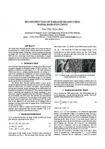
ABSTRACT Computerized ionospheric tomography (CIT) is a method to investigate ionosphere electron density in two or three dimensions. This method provides a flexible tool for studying ionosphere. Earth based receivers record signals transmitted from the GPS satellites and the computed pseudorange and phase values are used to calculate Total Electron Content (TEC). Computed TEC data and the tomographic reconstruction algorithms are used together to obtain tomographic images of electron density. In this study, a set of basis functions and reconstruction algorithms are used to investigate best fitting two dimensional tomographic images of ionosphere electron density in height and latitude for one satellite and one receiver pair. Results are compared to IRI-95 ionosphere model and both receiver and model errors are neglected. 1. INTRODUCTION Ionospheric electron density (IED) image can be reconstructed from TEC values obtained from recordings of GPS receivers. The Earth based receivers record pseudorange and phase of two signals, whose frequencies are 1575.42 MHz and 1227.60 MHZ [1]. TEC is defined as a line integral of the electron density between GPS satellite and GPS receiver. TEC is the number of electrons included in cylinder with 1 m2 cross-section. Since TEC carries information on time and position variability of the ionosphere, it is widely used in ionospheric research. The group delay and phase fluctuation of the two signals transmitted from the satellites are proportional to TEC values [2]. TEC computations can be performed with different precision levels and different methods such as Time Delay Measurement or Differential Phase Forward Measurement. Tomographic reconstruction algorithms and calculated TEC values are used together to reconstruct ionosphere electron density image for a relevant scenario which is also a function of the receiver and satellite geometry. Figure 1 shows a simplified example ionospheric tomography system.
Satellite N1 N3 d3
d1
N2 d4 N4 Receiver
Figure 1. Sample Ionospheric Tomography System
In the above system, Nk indicates electron density in the pixel, dk indicates the length of ray occupied by the pixel. For these parameters, k takes a value between 1 and 4, and TEC value for the ray can be given as TEC= c (d1 × N1 + d 3 × N 3 + d 4 × N 4 ) + err
(1)
In (1), c is an estimate constant and err is the error term. CIT method is based on this basic concept. 2. IONOSPHERIC MEASUREMENTS AND RECONSTRUCTION ALGORITHMS Ionospheric tomography poses some extra physical limitations in the performance of the tomographic algorithms. In CIT, receivers are placed on spherical Earth surface at any possible location, not necessarily equidistant from each other. The number of GPS satellites are limited and they trace a path over the receiver not designed for CIT. This causes limited observation angle and limited number of projection samples can be collected. Due to these limitations, conventional tomographic imaging methods have to be modified to overcome the low performance. To overcome these difficulties, CIT methods which include a priori information about the ionosphere are developed [3]. In these methods, ionosphere electron density is modelled as a linear combination of two dimensional basis functions. Two dimensional basis functions are obtained as the product of the vertical and horizontal basis functions. Legendre polynomials or Fourier poly-
nomials are preferred as horizontal basis functions [1,3], and vertical basis functions are usually generated from the forward ionosphere models such as International Reference Ionosphere (IRI) [3]. By using the vertical profiles from a selected forward model, vertical basis functions can be calculated. Computational complexity of these methods is proportional the number of horizontal basis functions, so selection of appropriate number of horizontal basis function is a critical parameter.
zontal basis functions are selected as Scaled Legendre polynomials, Cut Legendre Polynomials and Haar basis functions [5]. Horizontal basis functions and vertical basis functions are used together to obtain two dimensional basis functions. SVD of the distribution in Figure 2 is used to obtain the vertical basis functions which is given in Figure 3.
Ionospheric tomography system is simulated with one GPS satellite and one receiver to collect two transmitted signals and compute TEC values. For each satellite position, a TEC value is calculated on each receiver that capture signals from this satellite and by using this TEC values, it is possible to create tomographic images of ionosphere electron density. In this measurement setup, each TEC value can be expressed as TEC = ∫N(s) ds L
(2)
and (2) is the line integral of N(s) along the path L. In this expression, N(s) is electron density and L is one of rays from satellite to receivers. This line integral definition is similar to the medical line integral definition given in [4]. Based on this definition, TEC value is a sample point in the tomographic projection obtained for the satellite position. In this paper, tomographic reconstruction algorithms such as Regularized Least Squares (RLS) [5], Truncated SVD (TSVD) [6] and Total Least Squares (TLS) [7], are implemented and reconstruction errors are presented. In this study, ionosphere is modeled as grid structure with 95 pixels on vertical line and 29 pixels on horizontal line. It is assumed that electron density in each pixel has uniform distribution. Ionospheric electron density over height-latitude plane is expressed as a serial expansion as given below: K
g(r,θ) ≈ ∑ x k φ k ( r , θ ) k =1
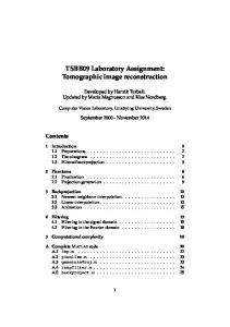
Figure 2. IRI-95 Electron Density Model. DATE: year, month, day Time: Hour Geographical Longitude Solar Zenith Angle/degree Dip (Magnetic Inclination)/degree Modip (Modified Dip)/degree Solar Sunspot Number Ionospheric-Effective Solar Index IG12
2003, 08, 5 15.5 LT 34 65.3 -60.62 -48.14 52.3 86.9
Table 1. IRI-95 Model Parameters
(3)
In (3), φ k ( r , θ ) = u m ( r ) v n (θ ) is a two dimensional basis function for k=m+(n-1)M, m=1,…,M; n=1,…,N, and u m (r ) is the vertical basis function obtained from IRI-95 model by SVD and the v n (θ ) is the horizontal basis function. In these expressions, K is number of total basis functions, M is number of vertical basis functions and N is number of horizontal basis functions. r is the height from sea level and it varies between 60 km to 1000 km. θ is the latitude in degrees. 3. MODEL IONOSPHERE AND BASIS FUNCTIONS In this paper, IRI-95 is selected as a reference ionosphere model and ionosphere cross-section for [–28° 28°] latitude interval for the parameters given in Table 1, is provided in Figure 2. It is assumed that the ionosphere is time invariant for each satellite positions and for each TEC calculations. Vertical basis functions are calculated by using the Singular Value Decomposition (SVD) over the IRI-95 model. Hori-
Figure 3. Vertical Basis Functions from IRI-95 Model. Figure 4, Figure 5 and Figure 6 show the horizontal basis functions for Haar, Scaled Legendre and Cut-Legendre, respectively. The Scaled-Legendre polynomials are obtained by scaling the standard Legendre polynomials between –28° and 28° latitudes.
4. RESULTS AND DISCUSSION The optimum number of basis functions is an important parameter in performance of the reconstruction algorithms. Reconstruction error can be defined as ε (N,M) =
Figure 4. First Four Haar Basis Functions Generated for [– 28° 28°] Latitude Interval.
Figure 5. Scaled and Orthonormalized Legendre Polynomial for [–28° 28°] Latitude Interval.
Gˆ ( N, M ) - G
(4)
G
where G is electron density matrix obtained from IRI-95 ˆ ( N, M ) is the model for [–28° 28°] latitude interval, and G reconstructed electron density matrix. Each column of G includes electron density variations according to height and is constituted by g(r,θ) given in (3). Due to this relation, first element of G is equal to g ( r1 , θ1 ) which is the sample for 1000 km and -28° degree. The error with respect to the number of horizontal basis function for RLS, TLS and TSVD reconstruction algorithms is given in Figure 7, Figure 8 and Figure 9 for Scaled Legendre, Cut-Legendre and Haar Wavelets as horizontal basis functions, respectively. From these figures, the optimum number of horizontal basis functions for each algorithm where M is set to 3, is determined as the point where error drops to a value where increasing the number of basis functions do not reduce the error further. In Table 3, the error norm, ε(Nopt,3), for total reconstruction is presented for various reconstruction algorithms and basis functions. Nopt is the optimum number of horizontal basis functions obtained from Figure 7, Figure 8 and Figure 9. In Figure 10, the reconstructed image for RLS algorithm and Cut Legendre basis is given.
ε(N,3)
Figure 7 Error Variations for Scaled Legendre polynomial
Figure 6. Cut and Orthonormalized Legendre Polynomial for [–28° 28°] Latitude Interval These polynomials are orthonormalized by Gram-Schmidt orthogonalization process. The Cut-Legendre is obtained by truncating the standard Legendre Function between –28° and 28° latitudes. Then the truncated polynomial is orthonormalized by Gram-Schmidt orthogonalization process. Haar basis functions are also mapped to [–28° 28°] latitude interval and x-axis is modelled as a distance between –28° and 28° latitudes in which the one degree is equal to 111 km.
ε(N,3)
Figure 8 Error Variations for Cut Legendre polynomial
basis functions used to ionospheric reconstruction. In Table 4, mathematical computations considered for all reconstruction algorithms are given. As seen from Table 4, RLS requires matrix product, matrix inversion and regularization procedure. Mathematical operations needed by matrix multiplication is order of n2 and lower bound is given by 2.5 n2 [8]. Matrix inversion requires 4n3/3 - n/3 multiplications/divisions and 4n3/3 - 3 n2 + n/6 additions/subtractions [9]. TLS algorithm needs SVD computations and the number of computations to compute the SVD of an mxn matrix is approximately 4mn2 - 4n3/3 if only the singular values are needed [10].
ε(N,3)
5. CONCLUSION Figure 9 Error Variations for Haar basis functions
In this paper, the performance of RLS, TLS and TSVD algorithms are compared for three different horizontal basis functions, namely Haar Wavelets, Scaled Legendre Polynomials and Cut-Legendre Polynomials. The electron density is modelled by the IRI-95 for [–28° 28°] latitude interval. Only one transmitter and one receiver is used in the simulated scenarios. It is observed that among all basis functions, the smallest number of horizontal basis is obtained by Haar Wavelets for all reconstruction algorithms, reducing the computational complexity. For the given scenario, for the reconstruction algorithm and basis function set, the total error is minimized for different pairs. It is expected that as the numbers of satellites and receivers are increased, the reconstruction error will be further reduced. REFERENCES
Figure 10. Reconstruted Image for TLS and Haar Wavelets RLS TLS TSVD
Haar Scaled-Legendre Cut-Legendre 28 32 32 28 54 32 28 32 32 Table 2. Number of Horizontal basis functions
RLS TLS TSVD
Haar Scaled-Legendre Cut-Legendre 0.2795 0.5860 0.1798 0.1813 1.4852 0.2319 0.2797 0.6116 0.1798 Table 3. ε(Nopt,3) for reconstruction algorithms
RLS TLS TSVD
Matrix product Matrix Inversion Regularization SVD Summations Divisions SVD Summations Divisions Table 4. Mathematical Operations for Algorithms
Given in Table 3, Scaled Legendre polynomial has the worst performance than Cut Legendre and Haar Basis functions. RLS and TSVD has same performance as expected from the mathematical details explained in [6]. In Table 2, the number of horizontal basis functions are given for reconstruction algorithms. As can be seen from Table 2, computational complexity for RLS with Cut Legendre is more than TLS with Haar basis functions due to the number of horizontal
[1] Jeffrey R. A., Steven J. F., Liu C. H., ''Ionospheric Imaging Using Computerized Tomography'', Radio Science, vol. 23, no. 3, pp. 299-307, May/June 1988. [2] Calais, E., Minster, J. B., ''GPS, Earthquakes, The Ionosphere and the Space Shuttle'', Physics Of The Earth and Planetary Interiors, vol. 105, pp. 167-181, 1998. [3] Sutton, E., Na, H., ''High Resolution Ionospheric Tomography Through Orthogonal Decomposition'', in Proceedings of ICIP-94., IEEE International Conference, 1316 Nov. 1994, vol. 2, pp. 148-152. [4] Kak, A. C., Slaney, M., Principles of Computerized Tomographic Imaging, IEEE Press, 1988. [5] Zhu, W., Wang, Y., Deng, Y., Yao, Y., Barbour , R. L., ''A Wavelet-Based Multiresolution Regularized Least Squares Reconstruction Approach for Optical Tomography'', IEEE Transaction on Medical Imaging, vol. 16, no. 2, pp. 210-271, April 1997. [6] Hansen, P. C., ''The truncated SVD as a method for regularization'', BIT, vol. 27, pp. 534-553, 1987. [7] Golub, G. H., Hansen, P. C., O’Leary, D. P., ''Tikhonov regularization and total least squares'', SIAM J. Matrix Anal. Appl., vol. 21, pp. 185-194, 2000. [8] Bshouty, N. H., “A Lower Bound for Matrix Multiplication’, SIAM Journal of Computing, vol. 18, pp. 759-765, 1989. [9] Burden, R. L, Faires, J. D., Numerical Analysis, Sixth Edition, Brooks/Cole Publishing Company, 1997. [10] Moon, T. K., Stirling, W. C., Mathematical Methods and Algorithms for Signal Processing, Prentice Hall, 2000.