TOMOGRAPHIC RECONSTRUCTION BASED ON. FLEXIBLE GEOMETRIC MODELS. K. M. Hanson, G. S. Cunningham, G. R. Jennings, Jr., and D. R. Wolf.
Proc. IEEE Int. Conf. on Image Processing, Vol. II, pp. 145-147, Austin, TX, November 13-16, 1994.
TOMOGRAPHIC RECONSTRUCTION BASED ON FLEXIBLE GEOMETRIC MODELS K. M. Hanson, G. S. Cunningham, G. R. Jennings, Jr., and D. R. Wolf Los Alamos National Laboratory, MS P940 Los Alamos, New Mexico 87545 USA {kmh, cunning, jennings}@lanl.gov ABSTRACT
the full posterior probability density function. The degree and type of warping is readily controlled through a judicious choice of the prior probability density function on the transformation parameters. In this paper a different tact is employed. Rather than try to warp a planar object to match the projection data taken of a lumen, or blood vessel, the lumen is modeled in terms of its outer boundary. The default shape for the cross section of the vessel is assumed to be a circle. Thus the circular border is given a slight amount of rigidity and allowed to flex (or warp) to match the data. Of course, the final choice of models should only be made after a thorough evaluation based on significant clinical experience.
When dealing with ill-posed inverse problems in data analysis, the Bayesian approach allows one to use prior information to guide the result toward reasonable solutions. In this work the model consists of an object whose amplitude is constant inside a flexible boundary. The flexibility of the boundary is controlled by through a distortion energy. We present an example of reconstruction of the cross section of a blood vessel from just two projections. 1.
INTRODUCTION
When very few projections are available, tomographic reconstructions are usually vastly underdetermined, so many solutions are possible. Bayesian methods of reconstruction can help identify the solution most similar to the characteristics of the object being imaged that are known a priori. The known properties of the object are incorporated in terms of prior probability density functions on the appropriate physical parameters. These methods can substantially improve the accuracy of reconstructions obtained from very limited data when good geometrical information is employed in the model [1, 2]. Previously we employed an approach in which the model for the object being reconstructed is allowed to alter its geometrical characteristics to accommodate the data by warping the coordinate system of the model onto the coordinate system of the reconstruction. This geometrical flexibility permits the reconstruction procedure to adapt the shape of the model to conform to the measurements. Within the Bayesian framework, the parameters needed to specify the coordinate transformation are determined as part of the overall estimation/reconstruction problem of finding the maximum of
2. BAYESIAN FORMULATION We represent the amplitudes of the N pixels of an image by a vector f of length N. We are given M discrete measurements that are linearly related to the amplitudes of the original image and assume that these measurements are degraded by additive noise. The measurements can then be represented by the vector g = Hf + n, where n is the random noise vector, and H is the measurement matrix. In computed tomography the elements of the jth row of H describe the weight of the contribution of each image pixel to the jth projection measurement. The Bayesian formulation is based on probabilities that, because they are a function of continuous parameters, are actually probability densities, designated by a small p(). From Bayes’ law, the negative logarithm of the posterior probability density is given by − log[p(f |g)] = φ(f ) = Λ(f ) + Π(f ) ,
(1)
where the first term comes from the likelihood p(g|f ) and the second term from the prior probability p(f ). Assuming additive Gaussian noise with a known covariance matrix Rn , the negative log(likelihood) is just half of chi-squared: − log[p(g|f )] = Λ(f ) = 12 χ2 =
Supported by the United States Department of Energy under contract number W-7405-ENG-36.
145
�T � � g − Hf R−1 n g − Hf . The second term Π(f ) comes from the prior probability density function. It should incorporate as much as possible the known characteristics of the types of objects under study. In the present context, the prior information being incorporated consists of the geometric or morphological nature of the object being reconstructed, to be discussed in the next section. The reconstruction procedure typically involves finding the image f that maximizes the posterior probability, called the MAP solution, or minimizes φ(f ). 1 2
�
density associated with bending is proportional to the square of the reciprocal of the radius of curvature κ: wbend = cbend κ2 = cbend (x� y �� − y � x�� ) , 2
where the primes indicate differentiation with respect to s and cbend is a constant. In some cases we may want to avoid the complete collapse of the border and the possible crossing over of opposite sides of the object. This goal can be reached by adding another term to W that provides a modest repulsive potential between all parts of the boundary.
3. A FLEXIBLE BOUNDARY MODEL
4. EXAMPLE
We model the object being reconstructed in terms of its boundary, which is assumed to be a closed curve. The interior of this boundary is assumed to have a constant amplitude, and the exterior amplitude is zero. The curve is given in terms of its original arc length, s: x = x(s) ; y = y(s). This boundary curve is considered to be flexible and stretchable. Thus the model depends only on the boundary, a curve in our 2D solution space. This model is different from the one explored previously [2], which involved a description that provided full 2D versatility. Flexible 1D curves in a 2D space may be thought of as splines, manifolds in differential geometry [3], or ‘snakes’ [4]. The flexible curve may be interpreted in terms of an analogous physical system, a closed loop of elastic material that undergoes distortion while being constrained to lie in the plane. Then the constraints placed on the curve correspond to the properties of the material being distorted, such as its stiffness. For materials obeying Hooke’s law, the strain energy density, found by integrating the stress with respect to the strain, is proportional to the square of the strain. The coefficients for bending and stretching are proportional to the corresponding effective elastic moduli of the fictitious boundary material. The selection of these coefficients should, of course, be made on the basis of the prior clinical knowledge of the shapes of actual lumina for the type of blood vessels under study. We use a Gibbs’ distribution for the prior probability on the flexing of the curve, which is proportional to exp(−W ), where W is the total strain energy
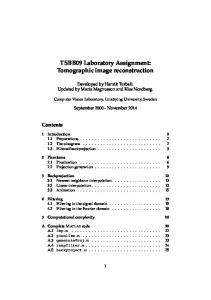
To demonstrate the proposed approach, we present a simple example of reconstruction from just two views. Figure 1 shows the original scene consisting of a simulated lumen or blood vessel. The images in this example are all 32 × 32 pixels in size. Two noiseless parallel projections of this object, one taken vertically and the other horizontally, are assumed to be available. The result of the Multiplicative Algebraic Reconstruction Technique (MART) [5], which is known [6] to converge to a maximum-entropy solution of the measurement equations, is predictably very poor. Assuming that the object is known to be roughly circular and that its amplitude is unity, the circle shown in the upperright (UR) panel is an appropriate default model. The prior effectively consists of this model, together with a contribution to Π based on the bending energy needed to deform the boundary from this shape. The resulting MAP solution (LR) is much better that the MART reconstruction. 5. THE BAYES INFERENCE ENGINE We are incorporating the previous ideas into an application that we call the Bayes’ Inference Engine (BIE). This application provides a convenient framework in which to deal directly with the geometry of objects, both in terms of flexible boundaries as shown here, and flexible interiors, as in [2]. The application is designed to allow one to easily change the description of how the measurements are modeled through a graphicalprogramming interface of the data-flow diagram [7]. The modular design of the BIE facilitates the calculation of the derivatives of φ with respect to all the variables in the object model, which are needed to find the minimum of φ [8]. Furthermore, a newly developed technique allows one to explore the reliability of the MAP solution by means of hands-on manipulation of the object model [9]. This technique is derived from
� Π(f ) ∝ W =
(wbend + wstretch ) ds ,
(3)
(2)
where the integral is over the arclength of the boundary s. The two energy density functions measure how much the curve is bent and stretched, respectively, relative to its initial default configuration. The strain energy 146
Duncan. Non-rigid motion models for tracking the left-ventricular wall. In A. C. F. Colchester and D. Hawkes, editors, Info. Processing in Med. Imag., pages 343–357. Springer-Verlag, 1991. [4] M. Kass, A. Witkin, and D. Terzopoulos. Snakes: active contour models. Inter. J. Comp. Vision, 1:321–331, 1988. [5] R. Gordon, R. Bender, and G. Herman. Algebraic reconstruction techniques for three-dimensional electron microscopy and x-ray photography. J. Theor. Biol., 29:471–481, 1970. [6] A. Lent. A convergent algorithm for maximum entropy image restoration, with a medical x-ray application. In R. Shaw, editor, Image Analysis and Evaluation, pages 45–57. Soc. of Photog. Scien. and Eng., New York, 1977. [7] G. S. Cunningham, K. M. Hanson, G. R. Jennings, Jr., and D. R. Wolf. An object-oriented implementation of a graphical-programming system. Medical Imaging: Image Processing, ed. M.H. Loew, Proc. SPIE, 2167:914–923, 1994.
Figure 1: Tomographic reconstructions based on two orthogonal projections of an original simulated lumen with a partial occlusion (upper-left). The result provided by the MART algorithm (lower-left) is very poor. The MAP reconstruction (lower-right), based on a default model (upper-right) with a flexible boundary defined by eight control points contacted with B-spline curves, is much better.
[8] G. S. Cunningham, K. M. Hanson, G. R. Jennings, Jr., and D. R. Wolf. An object-oriented optimization system. Proc. IEEE Int. Conf. Image Processing, III:826–830, 1994. [9] K. M. Hanson, G. S. Cunningham, and D. R. Wolf. The hard truth. In J. Skilling, editor, Maximum Entropy and Bayesian Methods, pages 157– 164. Kluwer Academic, 1996.
the suggestion in Sec. 3 of interpreting φ as a physical potential, the derivatives of which represent forces. The accuracy of the MAP solution is probed by perturbing the relevant model parameters and determining the force with which the solution pulls back. ACKNOWLEDGEMENTS We happily acknowledge instructive discussions with Jerry U. Brackbill and James Gee on methods of geometrical warping. Allen Mathews provided the computer code to fill the interior of the spline contours. 6. REFERENCES [1] K. M. Hanson. Bayesian and related methods in image reconstruction from incomplete data. In Henry Stark, editor, Image Recovery: Theory and Application, pages 79–125. Academic, Orlando, 1987. [2] K. M. Hanson. Bayesian reconstruction based on flexible prior models. J. Opt. Soc. Amer., A10:997– 1004, 1993. [3] A. A. Amini, R. L. Owen, P. Anandan, and J. S. 147