Algorithms and frameworks for stream mining and

Algorithms and frameworks for stream mining and knowledge discovery on Grids

Salvatore Orlando, Raffaele Perego, Claudio Silvestri {orlando|silvestri}@dsi.unive.it [email protected] ISTI-CNR, Pisa, Italy Antonio Congiusta, Domenico Talia, Paolo Trunfio {acongiusta|talia|trunfio}@deis.unical.it Universit`a della Calabria, Rende (CS), Italy

CoreGRID Technical Report Number TR-0046 July 4, 2006

Institute on Knowledge and Data Management CoreGRID - Network of Excellence URL: http://www.coregrid.net

CoreGRID is a Network of Excellence funded by the European Commission under the Sixth Framework Programme Project no. FP6-004265

Algorithms and frameworks for stream mining and knowledge discovery on Grids Salvatore Orlando, Raffaele Perego, Claudio Silvestri {orlando|silvestri}@dsi.unive.it [email protected] ISTI-CNR, Pisa, Italy Antonio Congiusta, Domenico Talia, Paolo Trunfio {acongiusta|talia|trunfio}@deis.unical.it Universit`a della Calabria, Rende (CS), Italy CoreGRID TR-0046

July 4, 2006

Abstract Many critical data mining (DM) applications, like intrusion detection or stock market analysis, require a nearly immediate result based on a continuous and infinite stream of data. Often we have to face the additional difficulty of mining multiple and distributed streams, so that it becomes mandatory to mine them by exploiting the resources close to data sources. In these cases, finding an exact solution is not compatible with the limited availability and capacity of computing, storing, and communicating resources, as well as with real time constraints. However, an approximation of the exact result is enough for most purposes. This report discusses a novel algorithm for approximate mining of frequent itemsets from multiple streams of distributed transactions using a limited amount of memory. The proposed algorithm is based on the computation of frequent itemsets in recent data and an effective method for inferring the global support of previously infrequent itemsets. Both upper and lower bounds on the support of each pattern found are returned along with the interpolated support. The resulting distributed framework for extracting patterns is suitable for running on a Grid. Since the technologies based on the Service Oriented Architecture (SOA) are now very popular for building the next generation Grid and Web, it is interesting to evaluate how these SOA technologies can be used to build a seamless distributed Grid system able to perform knowledge extraction and data mining. SOA can, in fact, supports the easy integration of algorithms, tools, and data sources, by also orchestrating specialized mining services like the ours. For all these reasons, in this report we outline the main features of the SOA services that are useful to build the Knowledge Grid, a novel framework for realizing distributed and composite knowledge discovery processes, by integrating Grid resources and (distributed and stream) data mining tools, also by supporting data management, and knowledge representation.

1

Introduction

This report discusses two novel results obtained in the field of distributed and stream data mining (DM). The former is concerned with a stream algorithm for approximate mining of frequent itemsets, APStream (Approximate Partition for Stream). We also propose an extension able to deal with this issue in more challenging cases. In particular, we also show that the proposed merge/interpolation framework devised for the stream case can seamlessly be extended to manage distributed streams in several ways. The latter result deals with a proposal of supporting a complete knowledge discovery process over emerging highly distributed platforms like computational Grids, by using technologies based on Service Oriented Architecture (SOA). This research work is carried out under the FP6 Network of Excellence CoreGRID funded by the European Commission (Contract IST-2002004265).

1

1.1

Frequent Patterns from Stream and Distributed Data

The stream and distributed data DM framework discussed in this report regards an important knowledge extraction analysis, known as Association Rule Mining (ARM) [3, 19]. ARM deals with the extractions of association rules from a database of transactions D. We are interested in the most computationally expensive phase of ARM, i.e., the Frequent Itemset Mining (FIM) one, during which the set F of all the itemsets that occurs in at least a user specified number of transactions is discovered. Those itemsets are named Frequent Itemsets. The computational complexity of the FIM problem derives from the exponential size of its search space P(I), i.e. the power set of I, where I is the set of items contained in the various transactions of D. A way to prune P(I) is to restrict the search to itemsets whose subsets are all frequent. The APriori algorithm [3], and other derived algorithms for non dynamic datasets, exactly exploits this pruning technique, based on the Apriori anti-monotonic principle. In a stream setting, new transactions are continuously added to the dataset. The infinite nature of stream data sources is a serious obstacle to the use of most of the traditional methods, since available computing resources are limited, whereas the amount of previously happened events is usually overwhelming. Thus, one of the first effects is the need to process data as they arrive, due to the impossibility of storing them. The results extracted evolve continuously along with data. In our case, since we adopt a landmark window model, these results refer to the whole data stream arrived so far, from a given past time (when we started collecting data) to the current time. Obviously, an algorithm suitable for stream data should be able to compute the ’next step’ solution on-line, starting from the previously known one and the current data, if necessary with some additional information stored along with the past solution. In our case, this information is the count of a significant part of frequent single items, and a transaction hash table used for improving deterministic bounds on supports returned by the algorithm. Unfortunately, even the apparently simple discovery of frequent items in a stream is challenging [6]. Some items, initially frequent, may eventually become infrequent. On the other hand, other items may appear initially in a sporadic way and then become frequent. Thus the only way to exactly compute the support of these items is to maintain a counter since the first appearance of each of them. This could be acceptable when the number of distinct items is reasonably bounded. If the stream contains a large and potentially unbounded number of spurious items, as in case of data with probabilities of occurrence that follow a Zipf’s law, like internet traffic data, this approach may lead to a huge waste of memory. In the first part of this report we discuss a stream algorithm for approximate mining of frequent itemsets, APStream (Approximate Partition for Stream). The infinite flow of data block in the stream is processed by considering past processed data and recent data as two partitions of transactions. Upon new data arrival, as many transactions as possible are buffered and processed in-core. The amount of buffered transactions obviously depends on their lengths, but also on the size of main memory available. The past approximate solution is then merged with the frequent pattern set obtained from recent data. Since past input transaction cannot be maintained, a second pass on the whole stream is impossible. We thus use an approximate support inference heuristic during the merge phase in order to improve the support accuracy. Both upper and lower bounds on the support of each pattern found are returned along with the interpolated support. Finally we propose an extension able to deal with this issue in more challenging cases, i.e. the mining of multiple and distributed streams of data. The resulting distributed framework for extracting patterns is suitable for running on a Grid.

1.2

Systems to support knowledge discovery processes

In order to support a complete knowledge discovery process over emerging highly distributed platforms like computational Grids, the main issue is the integration of two main requirements: synthesizing useful and usable knowledge from data, and performing complex large-scale computations leveraging the Grid infrastructure. Such integration must pass through a clear representation of the knowledge base used in order to translate moderately abstract domainspecific queries into computations and data analysis operations able to answer such queries by operating on the underlying systems [7]. Whereas some high-performance parallel and distributed data mining systems have been proposed [27] - see also [8] - there are few research projects attempting to implement and/or support knowledge discovery processes over computational Grids. Among them, the Knowledge Grid [9] is a framework for implementing knowledge discovery tasks in a wide range of high performance distributed applications. The Knowledge Grid offers to users high-level abstractions and a set of

CoreGRID TR-0046

2

services by which is possible to integrate Grid resources to support all the phases of the knowledge discovery process, as well as basic, related tasks like data management, data mining, and knowledge representation. The main issues investigated and solved by the Knowledge Grid is the definition/standardization of metadata, semantic presentation, and protocols for realizing discovery services and information management. Another important topic is the exploitation of data access and integration components, since data to be used for our mining process can be not only stored in distributed sites, but can also have different formats and associated metadata. Finally, knowledge discovery procedures typically require to create and manage complex, dynamic, multi-step workflows. At each step, data from various sources can be moved, filtered, integrated and fed into a data mining tool. Since current research activity on the next generation Grid and Web is focusing on designing and implementing its mechanisms following the Service Oriented Architecture (SOA) model, we have to choose a SOA-based technology to develop such system. Current research activity on the Knowledge Grid, which is the main subject of the second part of this report, is thus focused on designing and implementing its mechanisms following the Service Oriented Architecture (SOA) model. In particular, the so-called Open Grid Services Architecture (OGSA) paradigm and the emerging Web Services Resource Framework (WSRF) family of standards are being adopted for implementing the Knowledge Grid services and mechanisms. These services will permit the design and orchestration of distributed data mining applications running on large-scale, OGSA-based Grids.

1.3

Organization of the report

The first part of this report deals with our proposed algorithms and tools to extract pattern from stream and as follows. Section 2.1 formally introduces the FIM problem on streams. Then Section 2.2 describes the APStream algorithm, and the Partition algorithm that inspired APInterp and APStream . Before presenting and discussing our experimental results in Section 2.4, we introduce, in Section 2.4.1, some similarity measures that we use in order to evaluate the quality of the approximate results. Section 2.5 surveys the main related works in the field. Finally, in Section 2.6 we discuss some interesting extensions of the proposed method. In the second part of our report we discuss Grid and SOA platforms for building knowledge discovery and DDM systems. Section 3.1 presents a background about the Knowledge Grid architecture. Then we outline the main features of the Knowledge Grid services by using OGSA and WSRF, and discuss design aspects, execution mechanisms, and performance evaluations. In particular, Section 3.2 discusses the SOA approach and its relationships with Grid computing, while Section 3.3 presents a WSRF-based implementation of the Knowledge Grid services.

2

Approximate Mining of Frequent Patterns from Stream and Distributed Data

In this first part of the report we discuss a stream algorithm for approximate mining of frequent itemsets, APStream (Approximate Partition for Stream), which exploits DCI [32], a state-of-the-art algorithm for FIM, as the miner engine for recent data. The APStream algorithm uses similar techniques that we have already exploited in APInterp [39], an algorithm for approximate distributed mining of frequent itemsets. Both APStream and APInterp use a computation method inspired by the Partition algorithm [36]. Partition relies on a horizontally partitioned dataset, and consists in independently computing local results from each partition, merging the local sets of frequent itemsets, and then recounting each potentially frequent pattern over the whole dataset to discover the global results. In order to extend this approach to a stream setting, blocks of data received from the stream are used as an infinite set of partitions. Others stream association mining algorithms, such as LOSSY COUNT [29] for frequent itemsets, use a similar approach with some variation. Obviously, all of them avoid recounting potentially frequent itemsets over the whole dataset, which is not feasible with streaming data. APStream applies the same heuristic used by the previously introduced APInterp algorithm. The infinite flow of data block in the stream is processed pairwise, using past processed data and recent data as two partitions. Upon new data arrival, as many transactions as possible are buffered and processed in-core. The amount of buffered transactions obviously depends on their lengths, but also on the size of main memory available. The past approximate solution is then merged with the frequent pattern set obtained from recent data. Since a second pass on the whole stream is impossible, we use an approximate support inference heuristic during the merge phase in order to improve the support accuracy. Along with each interpolated support value, this method CoreGRID TR-0046

3

yields a pair of deterministic upper and lower bounds. The proposed inference heuristic can be easily replaced with a different one, more complex or better fitting a particular application context. In particular, our method is based on a simple, yet effective, interpolation schema based on the knowledge of the supports of the sub-patterns of a given infrequent pattern. Despite its simplicity, it entails good approximation results in experimental evaluation. So we expect that, for specific application contexts, a more focused inference method also based on domain knowledge would yield even better results. In data streams, the underlying data distribution may change. Hence the models built on old data might become inaccurate. This problem, known as concept drift, complicates the task of interpolating the count of past occurrences of a given pattern. The method we propose is in some way concept drift resilient, in particular when the drift concerns only the single item probability distributions and not the joint distributions. In Section 2.6, we propose an extension able to deal with this issue in more challenging cases.

2.1

The problem

In this section we formally define the FIM problem in both non-evolving databases and stream ones. Definition 1. (T RANSACTION DATASET ) Let I = {i1 , . . . , im } be a set of items. A non-evolving transaction dataset D is a collection of input sets or transactions: D = {t| t = (tid, t)}, where tid is a transaction identifier, and t = {i1 , . . . , ik } ⊆ I is a set of distinct items. The size D is the number n of transactions contained in D, i.e., n = |D|. The support of an itemset is a measure of its interestingness as a pattern, and is based on its frequency. Definition 2. (S UPPORT OF AN ITEMSET ) Let p ⊆ I be an itemset. The support σ(p) of itemset p in dataset D is defined as σ(p) = |{(tid, t) ∈ D | p ⊆ t}| i.e., the number of transactions in D that contain pattern p. The relative support sup(p) of pattern p is instead expressed as a fraction of transactions: sup(p) =

σ(p) |D|

Even if a transaction represents a set of items, with no particular order, it is convenient to assume that there exists some kind of total order R among them. Such order makes unequivocal the way in which an itemset is written, e.g., if we adopt an alphanumeric order we cannot write {B, A} since the correct way is {A, B}. Definition 3. (F REQUENT I TEMSET M INING ) Let minsup be a user chosen threshold. An itemset p is frequent in D if its support σ(p) is not less than σmin = minsup · |D|, i.e., if sup(p) > minsup. A k-itemset is a pattern composed of k items, Fk is the set of all frequent k-itemsets, and F is the set of all frequent itemsets. The Frequent Itemset Mining (FIM) problem consists in discovering F in D. In a stream setting, since new transactions are continuously added to the dataset, we need a notation for indicating that a particular dataset or result refers to a particular part of the stream. To this end, we write the interval as a subscript after the entity. Definition 4. (T RANSACTION S TREAM DATASET ) Let I = {i1 , . . . , im } be a set of items. A transaction data stream D is an infinite sequence of input sets or transactions: D = {t| t = (bid, tid, t)} where t = {i1 , . . . , ik } ⊆ I is a set of distinct items, while tid and bid are monotonically increasing identifiers, which are respectively associated with single transactions and blocks. The block identifier bid is chosen at reception time. In particular, all the transactions labeled with the same bid=i arrived before all the transactions labeled with bid=i+1. The transactions in the ith block, denoted as Di , are processed at the same time. The notation D[i,j) , i < j, identifies the part of the stream containing only the transactions whose bids are included in the interval [i, j), i.e., i ≤ bid < j. CoreGRID TR-0046

4

Thus D[1,j] denotes the part of the stream from the starting block until block j. If the j th block is the current one, and the notation is not ambiguous, we will just write D instead of D[1,j] . Due do the continuous evolution of datasets, in a stream settings a solution to the FIM problem must be tied to a part of the stream, indicated as a block interval D[i,j] . Depending on the part of stream involved, the problem presents different challenges, and is named differently. In particular, the landmark model [29, 26] considers the entire stream, the sliding window model [10] refers to its most recent part, and, finally, the tilted-time window model [22], is obtained by composing several distinct sliding windows, in order to maintain multiple time-granularities. In this report we discuss an algorithm for the solution of the FIM in the landmark model. We formally introduce this problem in the following. Definition 5. (F REQUENT I TEMSET M INING IN DATA S TREAMS ) Let minsup be a user chosen threshold. An itemset p is frequent in D[1,i] if its support σ[1,i] (p) is not less than σmin[1,i] = minsup · |D[1,i] |. A k-itemset is a pattern composed of k items, Fk[1,i] is the set of all frequent k-itemsets, and F[1,i] is the set of all frequent itemsets. The problem of Frequent Itemset Mining (FIM) in Data Streams consists in discovering F[1,i] in D[1,i] , for increasing values of i.

2.2

The Partition algorithm and its extensions

The APStream (Approximate Partition for Stream) algorithm used similar technique already used in our algorithm APInterp [39] for approximate mining of frequent itemsets in a distributed setting. Both algorithms are inspired by Partition [36], a sequential algorithm which divides the dataset into several partitions processed independently, and then merges the local solutions to produce the global result. In this report we will also use the terms local and global, as referred to stream input data or associated results. Local indicates something just concerning a contiguous part of the stream, hereinafter called a block of transactions, whereas global indicates something pertaining to the whole stream seen so far. In this section we will describe the Partition algorithm and its na¨ıve distributed and streaming versions, which we have used as a starting point for designing our approximate algorithms. 2.2.1

The original Partition algorithm

The basic idea exploited by Partition is the following: if the dataset is divided into several partitions, then each globally frequent itemset must be locally frequent in at least one partition. This guarantees that the union of all local solutions is a superset of the global solution. Partition sequentially reads the dataset, one partition at a time. For each partition it extracts the locally frequent itemset, and adds them to a set of potential globally frequent itemsets. After this phase, the result set contains every globally frequent itemset, mixed with several infrequent ones (false positives). Thus the dataset is read again, counting the exact occurrences of each candidate pattern, i.e., the ones that turned out to be frequent in only a proper subset of all the dataset partitions. At the end of the second scan all the infrequent patterns are removed, so that the result set only contains the FIM problem solution. 2.2.2

The Distributed Partition algorithm

Obviously, Partition can be straightforwardly implemented in a distributed setting with a master/slave paradigm [31]. Each slave becomes responsible of a local partition, while the master performs the sum-reduction of local counters (first phase) and orchestrates the slaves for computing the missing local supports for potential globally frequent patterns (second phase) to remove patterns having global support less than minsup (false positive patterns collected during the first phase). While the Distributed Partition algorithm gives the exact values for supports, it has pros and cons with respect to other distributed algorithms. The pros are related to the number of communications/synchronizations: other methods like count-distribution [23, 43] require several communications/synchronizations, while the Distributed Partition algorithm only requires two communications from the slaves to the master, a single message from the master to the slaves and synchronization after the first scan. The cons are concerned with the size of the messages exchanged, and the possible additional computation performed by the slaves when the first phase of the algorithm produces many false positives. Consider that, when low absolute minimum supports are used, it is likely to produce a lot of false positives due to data skew present in the various dataset partitions [35]. This has a large impact also on the cost of the second

CoreGRID TR-0046

5

phase of the algorithm: most of the slaves will participate in counting the local supports of these false positives, thus wasting a lot of time. A na¨ıve technique to work around this problem is to stop Distributed Partition after the first-pass. We call the algorithm that adopts this simple technique Distributed One-pass Partition. So, in Distributed One-pass Partition each slave independently computes locally frequent patterns and sends them to the master which sum-reduces the support for each pattern, and writes in the result set only the patterns having the sum of the known supports not less than minsup · |D|. Distributed One-pass Partition has obvious performance advantages over Distributed Partition. On the other hand, it yields a result which may be approximate, since it is possible that some globally frequent pattern occurs in a partition where it resulted to be locally infrequent, so that its local support count is unknown. In several cases this may cause the erroneous omission of globally frequent patterns. However, Distributed One-pass Partition ensures that at least the number of occurrences reported for each returned pattern exists. 2.2.3

The Streaming Partition algorithm

The infinite sequence of blocks of data that arrive from the data stream can be considered as an infinite set of partitions. This allows us to adopt the Distributed Partition approach also in a stream setting. Since the stream is infinite, however, it is impossible to collect and merge the results obtained from the various blocks. Thus the partial results must be merged repeatedly, and each time the result set needs to be updated. A block of data is processed as soon as ”enough” transactions are available, and the local result set of the current block is merged with the previous approximate result set, which refers to the past part of the stream. Unfortunately, due to memory constraints, in the stream case only recent raw data – i.e., the last block of transactions – can be maintained available for processing. Thus, in this case we can perform a second scan of them to check the support count of frequent patterns that resulted to be frequent in the past, but that are locally infrequent in the current block. Only the partial results extracted so far from previous blocks of the stream, plus some other additional information, can be available for determining the global result set, i.e. the frequent itemsets and their supports. Therefore, in the stream case it is impossible to perform a second scan on the past data to check the support count of a pattern that is locally frequent in the current block Dj , but that resulted infrequent in the past stream D[1,j) . A na¨ıve technique to work-around this problem is to keep in the global result set only those patterns having the sum of the known supports not less than minsup · |D[1,j] |. We call the algorithm that adopts this simple technique Streaming Partition. The known support counts are only the ones corresponding to those blocks in which the patterns resulted to be locally frequent. The first time an itemset x is reported, its support count corresponds to the support computed in the current block. In case it appearedPpreviously, this means introducing an error. If Di is the first block where x is frequent, then this error can be at most b∈[1,i) (σminb − 1).

2.3

The AP algorithm family

The two na¨ıve algorithms discussed above for distributed and stream settings, both inspired by Partition, have serious shortcomings. In particular, the weakness of Streaming Partition is common to several other stream FIM algorithms. When a previously ignored pattern becomes interesting, its exact support is largely underestimated. In order to overcome this issue, we propose a general framework that corrects the known supports of itemsets that result frequent in the current block of transactions, by using an interpolation schema based on other knowledge gathered from past data. The kind of interpolation used can be substituted seamlessly, in order to better fit the particular application context. In this article and in our previous works [39] we have used a really simple, yet effective, interpolation based on the reduction factor with respect to the supports of the subsets of the considered pattern. The APStream algorithm is derived from the distributed algorithm APInterp [39], using a method similar to the one used to build Streaming Partition from Distributed Partition. In the following subsection we will quickly describe APInterp , than we will introduce the APStream algorithm. 2.3.1

The APInterp algorithm

One of the most evident issues in Distributed Partition is the generation of several false positives, which in turn cause an increment of both resource utilization and execution time, especially when data skew between data partitions is high. The APInterp algorithm addresses this issue by means of global pruning based on good approximate knowledge of the global F2 : each locally frequent k-pattern which contains a globally non-frequent 2-pattern will be locally

CoreGRID TR-0046

6

removed from the set of frequents patterns before sending it to the master, and generating the next k + 1-candidate patterns. On the other hand, Distributed One-pass Partition uses a very conservative estimate for the support of patterns, since it always chooses the lower bounds (known support counts) to approximate the results. This causes underestimated support values, but also several false negatives, often for those patterns whose global supports are close to the threshold. The data skew, indeed, might cause a globally frequent k-pattern x to result infrequent on a given partition Di only. In other words, since σi (x) < minsup · |Di |, x will not be returned as a frequent pattern by the ith slave. As a consequence, the master of Distributed One-pass Partition cannot count on the knowledge of σi (x), and thus cannot exactly compute the global support of x. Unfortunately, in Distributed One-pass Partition, the master might P also deduce that x is not globally frequent, because j,j6=i σj (x) < minsup · |D|. In order to limit this issue, in APInterp the master infers an approximate value for this unknown σi (x) by exploiting an interpolation method. The master bases its interpolation reasoning on the knowledge of: • the exact support of single items in each partition; • the reduction factor r(x) with respect to the known supports of the items and subsets contained in the considered pattern x. Note that the support of some subset of x in a partition could be unknown too. This mean that it has been interpolated and discarded because globally infrequent during the k − 1 iteration, otherwise an approximation of its support would be known. In this case x can be discarded as well. The master can thus deduce the unknown support σi (x) on the basis of r(x), in turn derived from the supports of x in those partitions Di where x resulted to be frequent. Figure 1 shows an overview of the data flows in the distributed APInterp algorithm.

Figure 1: APInterp overview. When the number of distributed dataset partitions is really high, the computation cost for collecting and merging the local solutions could become considerable, since the complexity of the merge operation is linear in the amount of input data. To limit this issue, the nodes can be organized in a hierarchy, where each node fetches and merges the results of its direct descendant, and returns the result of the merge to the parent node. 2.3.2

The APStream algorithm

The streaming algorithm we propose in this report, APStream , tries to overcome some of the problems encountered by Streaming Partition and other similar algorithms for association mining on streams, when the data skew between CoreGRID TR-0046

7

σ[1,i) (x) Known Known

σi (x) Known Unknown

Unknown

Known

Action σ[1,i] (x) = σ[1,i) (x) + σi (x). Recount support σi (x) on recent, still available, data. Then σ[1,i] (x) = σ[1,i) (x) + σi (x). interp Interpolate past support σ[1,i) (x). interp Then σ[1,i] (x) = σ[1,i) (x) + σi (x).

Table 1: APStream : Computing the support of x in the whole data stream D[1,i] . different incoming blocks is high. This skew might cause a globally frequent itemset x to result infrequent on a given data block Di . In other words, since σi (x) < minsup · |Di |, x will not be found as a frequent itemset in the ith block. As a consequence, we will not be able to count on the knowledge of σi (x), and thus exactly compute P the support of x. Unfortunately, Streaming Partition might also deduce that x is not globally frequent, because j,j6=i σj (x) < minsup · |D|. APStream addresses this issue in different ways, as summarized in Table 1. In particular, the table shows all the possible cases regarding the knowledge of σ(x) on the current block Di and the previous part of the stream D[1,i) . The first case is the simplest to handle: the new support σ[1,i] (x) will be the sum of σ[1,i) (x) and σi (x). The second one is similar, except that we need to look at recent data for computing σi (x). The key difference with Streaming Partition is the handling of the last case. APStream , instead of supposing that x never appeared in the past, tries to interpolate σ[1,i) (x). The interpolation is based on the knowledge of: • the exact support of each item in D[1,i) (or, optionally, just the approximate support of a fixed number of the most frequent items); • the reduction factors r(x) of the support count of subsets of x in the current block with respect to its interpolated support over the past part of the stream. th

i

The algorithm will thus infer the unknown support σ[1,i) (x) of itemset x on the part of the stream preceding the block as follows: interp σ[1,i) (x) = σi (x) · r(x)

where µ µ ¶¶ σ[1,i) (item) σ[1,i) (x r item) r(x) = minitem∈x min , σi (item) σi (x r item)

(1)

The rationale of Equation (1) is that, given two itemsets x and x0 , x0 ⊂ x, if the exact value of σ[1,i) (x) is unknown, interp its interpolated value σ[1,i) (x) is approximated by using the following proportion: interp σi (x) : σi (x0 ) = σ[1,i) (x) : σ[1,i) (x0 )

so that interp σ[1,i) (x) = σi (x) ·

σ[1,i) (x0 ) σi (x0 )

Note that also σ[1,i) (x0 ) might be an approximate value previously interpolated. Given a k-itemset x, the reduction factor r(x) defined by Equation (1) is thus computed by considering all x0 , 0 x ⊂ x, such that x0 is either one of the single items belonging x, or a k − 1-itemset set-included in x. Finally, the value chosen for r(x) is the minimum one. Note that, since the merge of the results is performed level-wise starting first from shorter itemsets, when we interp try to approximate σ[1,i) (x), the exact or approximate value of σ[1,i) (x r item) must surely be known or already interpolated, for all item ∈ x. This is because all the k−1-itemsets included in x must be globally frequent. Otherwise, x could not be a valid candidate. Figure 2 shows an overview of the data flows in the APStream algorithm. CoreGRID TR-0046

8

Figure 2: APStream overview. x {A,B,C} {A,B } {A,C } {B,C } {A } {B } {C } {}

σi (x) 6 8 12 10 17 14 18 40

σ[1,i) (x) ? 50 30 100 160 140 160 400

σ[1,i) (x) σi (x)

6.2 2.5 10 9.4 10 8.9 -

Table 2: Sample supports and reduction ratios. Example of interpolation. Suppose that we have received 440 transactions so far, and that 40 of these are in the current block Di . The itemset x = {A, B, C}, briefly indicated as ABC, is locally frequent, whereas it was infrequent in previous data. Table 2 reports the support of every subset involved in the computation. The first columns contains the itemsets, the second and third columns contain the known supports of the patterns in the current block Di and in the past part of the stream D[1,i) . Finally, the last column shows the reduction factor implied by each pattern. According to Equation (1), the algorithm chooses the reduction factor r(x) for x = {A, B, C} by considering all σ (x0 ) the itemsets x0 , x0 ⊂ x, of size one and two. In this case the chosen minimum ratio [1,i) σi (x0 ) is 2.5, corresponding to the subset x0 = {A, C}. Since in Di the support of x = {A, B, C} is σi (x) = 6, the interpolated support will be interp σ[1,i) (x) = 6 · 2.5 = 15. It is worth remarking that this method works if the support of larger itemsets decreases similarly in most parts of the stream, so that a reduction factor (different for each itemset) can be used to interpolate unknown values. Finally interp note that, as regards the interpolated value above, we expect that the following inequality should hold: σ[1,i) (x) < minsup · |D[1,i) |. So, if we obtain it is not satisfied, this interpolated result should not be accepted. If it was true, the exact value σ[1,i) (x) should have already been found. Hence, in those few cases where the above inequality does not interp hold, the interpolated value will be: σ[1,i) (x) = (minsup · |D[1,i) |) − 1. Implementation. We can finally introduce the pseudo-code of APStream . As in Streaming Partition the transactions are received and buffered. DCI, the algorithm used for the local computations, exactly knows the amount of transactions that can be processed in-core. Thus we can use this knowledge in order to maximize the size of each block of transactions processed at a time. Since frequent itemsets are processed sequentially and can be offloaded to disk, we can ignore the memory occupied by the mined results. Figure 3 contains the pseudo-code of APStream . For the sake of simplicity we will neglect the quite obvious

CoreGRID TR-0046

9

main loop with code related to buffering, and concentrate our attention on the processing of each data block. The interpolation formula has been omitted too for the same reason. processBlock(buf f er, globF req) locF req[1] = ; k = 2; while size(locF req[k − 1]) >= k do locF req[k] = computeF requent(k, locF req, globF req); commitInsert(k, locF req, globF req); end while end; commitInsert(k, locF req, globF req) for all pat in globF req[k] and not in locF req[k] do if then end if end for end; computeFrequent(k, locF req, globF req) < compute local frequent itemsets > for all pat locally f requent do if then end if end for return Fk ; end;

Figure 3: APStream pseudo-code. Each block is processed, visiting the search space level-wise, for discovering frequent itemsets. In this way itemsets are sorted according to their length and the interpolated support for frequent subpatterns is always available when required. The processing of itemsets of length k is performed in two steps. First frequent itemsets are computed in the current block, and then the actual insertion into the past set of frequent itemsets is carried out. When a pattern is found to be frequent in the current block, its support on past data is immediately checked: if it was already known then the local support is summed to previous support and previous bounds. Otherwise a support and a pair of bounds are inferred for past data, and summed to the support in the current block. In both cases, if the resulting support passes the support test, the pattern is queued for insertion. After every locally frequent itemset of length k has been processed, the support of every previously known itemset which, on the other hand, resulted to be locally infrequent must be computed on recent data. Itemsets passing the support test are queued for insertion too. Then the pre-inserted itemsets in the queue are sorted and the actual insertion takes place. 2.3.3

Tighter bounds

As a consequence of using an interpolation method to guess an approximate support value in the past part of the stream, it is very important to establish some bounds on the support found for each pattern. In the previous subsection we have already indicated a pair of really loose bounds: each support cannot be negative, and if a pattern was found infrequent in the past data D[1,i) , then its interpolated support should be less than minsup · |D[1,i) |. This criteria is completely true for a non-evolving distributed dataset (distributed frequent pattern mining). In the stream case, however, the results are approximate and may be affected by false negatives. When a pattern is erroneously discarded as infrequent, its future upper bounds might be underestimated. Anyhow, this issue concerns just a limited number of patterns and, also in these cases, the bounds represent a useful approximation of the exact ones. Bounds based on pattern subset. The first bounds that interpolated supports should obey, derive from the Apriori property: no set can have a support greater than those of any of its subset. Since recent results are merged level-wise with previously known ones, the interpolation can exploit already interpolated subset support. When a subpattern is missing during interpolation, it means that it has been examined during a previous level and discarded. In this case all

CoreGRID TR-0046

10

of its superset may be discarded as well. The computed bound is thus affected by the approximation of past results: an itemset with an erroneous support will affect the bounds for each of its superset. To avoid this issue it is possible to compute the upper bound for an itemset x using the upper bounds of its sub-patterns instead of their support. In this way the upper bounds will be weaker, but there will be less false negatives due to erroneous bounds enforcement. Bounds based on transaction hash. In order to address the issue of error propagation in support bounds we need to devise some other kind of bounds, which are computed exclusively from received data, and thus are independent of any previous results. Such bounds can be obtained using inverted transaction hashes. The technique discussed below was first introduced in the algorithm IHP [25], an association mining algorithm, where it is used for finding an upper bound for the support of candidates in order to prune infrequent ones. As we will show, this method can also be used for lower bounds. The key idea is to use a number H of arrays of item counters where each array is associated with a disjoint set of input transactions. When a transaction t = (bid, tid, t) is processed, we only modify the counters in the hth array, where h is the result of a hash function applied to tid. Since tids are consecutive integer numbers, a trivial hash function, like hf (tid) = tid mod H, will guarantee an equal distribution of transactions among all hash bins. Thus, when the transaction t = (bid, tid, t) is processed, we update the array associated with the current tid (∀item ∈ t) Counth [item] + + where h = tid mod H. Let H = 1, i.e., a single array of counters is used. Let A and B be two items, and Count0 [A] and Count0 [B] the associated counters, i.e. Count0 [A] and Count0 [B] are the number of occurrences of items A and B in the whole dataset. According to the Apriori principle σ({A, B}) 6 min(Count0 [A], Count0 [B]) Furthermore we are able to indicate a lower bound for the same support. Let n be the total number of transactions n. We know from the inclusion/exclusion principle that σ({A, B}) > max(0, Count0 [A] + Count0 [B] − n) In fact, if n − Count0 [A] transactions does not contain the item A, then at least Count0 [B] − (n − Count0 [A]) of the Count0 [B] transactions containing B will also contain A. Suppose that n = 30, Count0 [A] = 18, Count0 [B] = 18. If we represent with an X each transaction supporting a pattern, and with a dot any other transaction, we obtain the following diagrams: Best case(ub(AB)= 18) Worst case(lb(AB)=6) A: XXXXXXXXXX XXXXXXXX.. .......... XXXXXXXXXX XXXXXXXX.. .......... B: XXXXXXXXXX XXXXXXXX.. .......... .......... ..XXXXXXXX XXXXXXXXXX AB: XXXXXXXXXX XXXXXXXX.. .......... .......... ..XXXXXX.. .......... supp 18 6

Then no more than 18 transactions will contain both A and B. At the same time at least 18 + 18 − 30 = 6 transactions will satisfy that constraint. Since each counter represents a set of transaction, this operation is equivalent to the computation of the minimal and maximal intersections of the tid-lists associated with the single items. Usually, however, H > 1. In this case, for each transaction tid, we will increment the counter array Counth [], where h = tid mod H. The bounds for the support of an itemset x are: σ(x)upper = σ(x)lower =

H−1 X h=0

H−1 X

Ã

h=0

min (Counth [item])

item∈x

max 0, nh −

X

! (nh − Counth [item])

item∈x

where nh is the total number of transactions associated with the hth hash value. Consider the same example discussed above, i.e. 30 transactions including items A and B, where σ(A) = 18 and σ(B) = 18. Let H = 3. Therefore nh = 10, for each h = 0, 1, 2. Suppose that Count0 [A] = 8, Count0 [B] = 7, Count1 [A] = 4, Count1 [B] = 5, Count2 [A] = 6, and Count2 [B] = 6. Using the same notation previously introduced we obtain: CoreGRID TR-0046

11

h=0 h=1 Best case Worst case Best case Worst case Best case A: XXXXXXXX.. XXXXXXXX.. A: XXXX...... XXXX...... A: XXXXXX.... XXXXXX.... B: XXXXXXX... ...XXXXXXX B: XXXXX..... .....XXXXX B: XXXXXX.... ....XXXXXX AB: XXXXXXX... ...XXXXX.. AB: XXXX...... .......... AB: XXXXXX.... ....XX.... supp 7 5 supp 4 0 supp 6 2

h=2 Worst case

Each pair of columns, which corresponds to a distinct h = 0, 1, 2, represents the transactions having a tid mapped into the corresponding location by the hash function. Note that the lower and upper bounds for σ({A, B}) are, respectively, 5 + 0 + 2 = 7 and 7 + 4 + 6 = 17. Note that these two bounds are stricter than 8 and 18, i.e., the ones obtained for H = 1. Both lower bounds and upper bounds computations can be extended recursively to larger itemsets. This is possible since the reasoning previously explained still holds if we considers the occurrences of itemsets instead of those of single items. The lower bound computed in this way will be often equal to zero in sparse datasets. Conversely, on dense datasets this method did prove to be effective in narrowing the two bounds.

2.4

Experimental evaluation

In this section we study the behavior of the proposed method. We run the APStream algorithm on several datasets using different parameters. The goal of these tests is to understand how similarities of the results vary as the stream length increases, how the hash based pruning is effective, and, in general, how dataset peculiarities and invocation parameters affect the accuracy of the results. Furthermore, we want to study how execution time evolves when the stream length increases. 2.4.1

Assessing accuracy.

The method we are proposing yields approximate results. In particular APStream computes itemset supports which may be slightly different from the exact ones. Thus the result set may miss some frequent itemset (false negatives), or include some infrequent itemset (false positives). Similarity measure. In order to evaluate the accuracy of the results, we need a measure of similarity between two pattern sets. A widely used one has been introduced in [35], and is based on support difference. Definition 6 (Similarity). Let A and B respectively be the reference (correct) result set and the approximate result set. supA (x) ∈ [0, 1] and supB (y) ∈ [0, 1], where x ∈ A and y ∈ B, correspond to the relative support found in A and B respectively. Note that since B corresponds to the frequent itemsets found by the approximate algorithm under observation, A − B thus corresponds to the set of false negatives, while B − A are the false positives. The Similarity is thus computed as P max{0, 1 − α ∗ |supA (x) − supB (x)|} Simα (A, B) = x∈A∩B |A ∪ B| where α > 1 is a scaling parameter, which increase the effect of the support dissimilarity. Moreover, α1 indicates the maximum allowable error on (relative) itemset supports. We will use the notation Sim() to indicate the default case for α, i.e. α = 1. This measure of similarity is thus the sum of at most |A ∩ B| values in the range [0, 1], divided by |A ∪ B|. Since |A ∩ B| 6 |A ∪ B|, similarity lies in [0, 1] too. When an itemset appears in both sets and the difference between the two supports is greater than α1 , it does not improve similarity, otherwise similarity is increased according to the scaled difference. If α = 20, then the maximum allowable error in the relative support is 1/20 = 0.05 = 5%. Supposing that the support difference for a particular itemset is 4%, the numerator of the similarity measure will be increased by a small quantity: 1 − (20 ∗ 0.04) = 0.2. When α is 1 (default value), only itemsets whose support difference is at most 100% contribute to increase similarity. On the other hand, when we set α to a very high value, only itemsets with a very similar supports in both the approximate and reference sets will contribute to increase the similarity measure.

CoreGRID TR-0046

12

It is worth noting that the presence of several false positives and negatives in the approximate result set B contributes to reduce our similarity measure, since this entails an increase in A∪B (the denominator of the Simα formula) with respect to A ∩ B. Moreover, if an itemset has an actual support which is slightly less than minsup but the approximate support (supB ) is slightly greater than minsup, similarity is decreased even if the computed support was almost correct. Two more classical result approximation measures are Precision and Recall, both originally introduced in the information retrieval context. The Precision is defined as the fraction of patterns contained in the solution that are actually frequent, i.e., it is the probability that a generic returned pattern will be actually frequent. The Recall is defined as the fraction of the total number of frequent pattern that are contained in the solution, i.e., it is the probability that a generic frequent pattern will be found by the algorithm. Both, however, does not consider the correctness of the support, but only the presence in the result set. This may be misleading, in particular when using a high minimum support threshold. On the other hand, a high similarity value ensure high Precision, high Recall, and limited differences between the actual support values and the discovered ones. Average support range. When bounds on the support of each itemset are available, an intrinsic measure of the correctness of the approximation is the average width of the interval between the upper bound and the lower bound [39]. Definition 7 (Average support range). Let B be the approximate result set, sup(x) the exact support for itemset x and sup(x)lower and sup(x)upper the lower and upper bounds on sup(x), respectively. The average support range is thus defined as: ASR(B) =

1 X sup(x)upper − sup(x)lower |B| x∈B

Note that, while this definition can be used for every approximate algorithm, how to compute sup(x)lower and sup(x)upper is algorithm specific. 2.4.2

Experimental data.

We performed several tests using both real world datasets, mainly from the FIMI’03 contest [1], and synthetic datasets generated using the IBM generator. We randomly shuffled each dataset and used the resulting datasets as input streams. Table 3 illustrates these datasets along with their cardinality. The datasets having the name starting with T are synthetic datasets, which mimic the behavior of market basket transactions. The sparse dataset family T20I8N5k has transactions composed, on average, of 20 items, chosen from 5000 distinct items, and includes maximal itemsets whose average length is 8. The dataset family T30I30N1k was generated with the parameters briefly indicated in its name. It is a moderately dense dataset, since more than 10,000 frequent itemsets can be extracted even with a minimum support of 30%. A description of all other datasets can be found in [1]. Kosarak and Retail are really sparse datasets, whereas all other the real world datasets used in experimental evaluation are dense. Table 3 also indicates, for each dataset, a short acronym that will be used in our charts for referring to it. Dataset accidents kosarak retail pumbs pumbs-star connect T20I8N5k T25I20N5k T30I30N1k

Reference A K R P PS C S2..6 S7..11 D1..D9

#Trans. 340183 990002 88162 49046 49046 67557 77302..3189338 89611..1433580 50000..3189338

Table 3: Datasets used in experimental evaluation.

CoreGRID TR-0046

13

Similarity(%) 100 95 90 85

%

80 75 70 A (minsupp= 30%, base mem=2MB) C (minsupp= 70%, base mem=2MB) P (minsupp= 70%, base mem=5MB) PS (minsupp= 40%, base mem=5MB) R (minsupp= 0.05%, base mem=5MB) K (minsupp= 0.1%, base mem=16MB)

65 60 55 1

2

4

8

16

Reletive available memory

Figure 4: Similarity as a function of available memory.

2.4.3

Experimental Results.

For each dataset and several minimum support thresholds, we computed the exact reference solutions by using DCI [32], the same FIM algorithm used as a building block for both APInterp and APStream . Then we ran APStream for different values of available memory and number of hash entries. The first test is focused on catching the effect of used memory on the behavior of the algorithm, when the block of transactions processed at a time is sized dynamically according to the available resources. In this case data are buffered as long as all the item counters, and the representation of the transactions included in the current block fit the available memory. Note that the size of all frequent itemsets, mined either locally or globally, is not considered in our resource evaluation, since they can be offloaded to disk if needed. The second test is somehow related to the previous one. In this case the amount of required memory is varied, since we determine a-priori the number of transactions to include in a single block, independently of the stream content. The typical use case for APStream matches the first test: the user chooses the support, while the other parameters are chosen adaptively, depending on the available system memory and data peculiarities. The second test, with this adaptive behavior disabled, has been inserted for the sake of completeness. Since the datasets used in the tests are quite different, in both cases we used really different ranges of parameters. Therefore, in order to fit all the datasets in the same plot, the number reported in the horizontal axis are relative quantities, corresponding to the block sizes actually used in each test. These relative quantities used in the chart are obtained by dividing the memory/block size used in the specific test by the smallest one for that dataset. For example, the series 50KB, 100KB, 400KB thus becomes 1, 2, 8. The plot in Figure 4 shows the results obtained in the fixed memory case, while the plot in Figure 5 corresponds to the case when the number of transactions per block is fixed. The relative quantities reported in both plots refer to different base values of either memory or transactions per blocks. These values are reported in the legend of each plot. In general when we increase the number of transactions processed at a time, either statically or dynamically on the basis of the memory available, we also improve the results similarity. Nevertheless the variation is in most cases small, and sometimes there is also a slightly negative trend, caused by the data dependant relationship between used memory and transactions per block. Indeed, a different amount of available memory entails a different division of the stream into blocks, having different sizes and starting points. Occasionally, this could worsen the similarity, in spite of a larger amount of available memory, as in the case of dataset PS in the plot in Figure 4. In our test we noted that choosing an excessively low amount of available memory for some datasets leads to performance degradation, and sometimes also to similarity degradation. The plot in Figure 6 shows the effectiveness of the hash-based bounds on reducing the Average Support Range (zero corresponds to an exact result). As expected, the improvement is evident only on more dense datasets. The last batch of tests makes use of a family of synthetic datasets, with homogeneous distribution parameters and

CoreGRID TR-0046

14

Similarity(%) 100 95 90 85

%

80 75 70 A (minsupp= 30%, base trans/block=10k) C (minsupp= 70%, base trans/block=4k) K (minsupp= 0.1%, base trans/block=20k) P (minsupp= 70%, base trans/block=8k) PS (minsupp= 40%, base trans/block=4k) R (minsupp= 0.05%, base trans/block=2k)

65 60 55 1

2

4

8

16

Relative transaction number per block

Figure 5: Similarity as a function of the number of transactions per block.

varying lengths. Each datasets is obtained from the larger dataset of the series by truncating it to simulate streams with different lengths. For each truncated dataset we computed the exact result set, used as reference value in computing the similarity of the corresponding approximate result obtained by APStream . The chart in Figure 7 plots both similarity and ASR as the stream length increases. We can see that similarity remains almost the same, whereas the ASR decreases when an increasing portion of the stream is processed. Finally, the plot in Figure 8 shows the evolution of execution time as the stream length increases. The execution time increases linearly with the length of the stream. Hence, the average time per transaction is constant if we fix the dataset and the execution parameters.

2.5

Related works

The Association Rule Mining (ARM) in transactional databases has been introduced in [3] and is one of the most popular topics in the KDD field [19, 21]. The Frequent Itemset Mining (FIM) is the most computationally expensive phase of ARM. Most FIM algorithms are based on the APriori [5] algorithm, which restricts the search to itemsets whose subsets are all frequent. APriori is a level-wise algorithm, since it examine the k-patterns only when all the frequent patterns of length k − 1 have been discovered. Several other algorithms based on the Apriori principle have been proposed. Some use the same level-wise approach, but introduce efficient optimizations, like a hybrid count/intersection support computation [32], or the reduction of the number of candidates using a hash based technique [34]. Others use a depth-first approach, either class based [43] or projection based [2, 24]. Others again use completely different approaches, based on multiple independent computations on smaller part of the dataset, like [36], or incremental computation on an adaptive sample of the data [35, 40, 18, 37]. Parallel (PDM) and distributed (DDM) data-mining are a natural evolution of data-mining technologies, motivated by the need of scalable and high performance systems. A number of parallel algorithms for solving the FIM have been proposed in the last years [4, 23]. Most of them can be considered parallelizations of the well-known Apriori algorithm. Zaki authored a good survey on ARM algorithms and relative parallelization schemas [42]. Agrawal et al. [4] proposed a broad taxonomy of the parallelization strategies that can be adopted for Apriori on distributed-memory architectures. The described approaches constitute a wide spectrum of tradeoffs between computation, communication, memory usage, synchronization, and the use of problem-specific information. The Count Distribution (CD) approach adopts the data-parallel paradigm, according to which the input transaction database is statically partitioned among the processing nodes, while the candidate set Ck is replicated. Count Distribution is an algorithm that can be realized in a distributed setting, since it based on a partitioned dataset, and also because the amount of information exchanged between nodes is limited. The other two methods proposed by Agrawal et al., Data and Candidate Distribution, require moving the dataset. Unfortunately in a distributed environment such dataset is usually already partitioned and distributed on distinct sites, and cannot be moved for several reasons, for example due to the low latency/bandwidth

CoreGRID TR-0046

15

Average support range(%) 5

A (minsupp= 30%) C (minsupp= 70%) K (minsupp= 0.1%) P (minsupp= 70%)

4.5 4 3.5

%

3 2.5 2 1.5 1 0.5 0 0

100

200

300

400

Hash entries

Figure 6: ASR as a function of the number of hash entries.

network that connects the sites. Several DDM FIM algorithms have been proposed, aimed at reducing the amount of communications involved in the Count Distribution method. FDM [13] constitutes an attempt to reduce the amount of communication entailed in the sum-reduction of the local counters in the CD parallelization of the Apriori algorithm. Schuster and Wolff [38] then introduced DDM, whose aim is to reduce the number of messages exchanged by FDM , since the number of messages exchanged by FDM in presence of non-homogeneity of database partitions quickly becomes similar to the ones exchanged by CD. The basic idea of DDM is to verify that an itemset is frequent before collecting its support from every party. The same authors extend the idea of DDM to a dynamic large scale P2P environment [41], i.e., a system based on utilizing free computational/storage resources on non-dedicated machines, where nodes can suddenly depart/join along with the associated database, thus modifying the global result of the computation. The exact discovery of frequent items in a stream of items may be a highly memory intensive problem [12]. Several relaxed versions of this problem exist, and some interesting ones were introduced in [12, 17, 28]. The techniques used for solving this family of problems can be classified into two large categories: count-based techniques [30, 17, 28, 29], sketch-based techniques [29, 12, 14, 15]. The first ones monitor a limited set of potentially ”interesting” items, using a counter for each one of them. In this case an error arises when an item is erroneously kept out of the set or inserted too late. The second family provides frequency estimation for every item by using a hash indexed vector of counters. In this case the risk of completely missing the occurrences of an item is avoided, at the cost of looser guarantees on the computed frequencies. The FIM problem on stream of transactions poses additional memory and computational issues due to the exponential growth of solution size with respect to the corresponding problem on streams of items. Two representative approximate algorithms are derived respectively from LOSSY COUNT [29] and FREQUENT [17, 28]. The first one is presented in [29], and is an almost straightforward extension of LOSSY COUNT. The second one is presented in [26], and, even if based on FREQUENT, is significantly different from it, since a property that ensures the correctness in the item case is no longer valid for itemsets. Both algorithms are affected by the issues previously described in the discussion of Streaming Partition, i.e., they do not consider the possible support count that a pattern could have, even if it has been reported as infrequent. LOSSY COUNT maintains the obvious upper bound that we also used, but no lower bound is exploited.

2.6

Extensions

The proposed interpolation framework for frequent pattern mining is based on the merge of partial results, using interpolation to replace missing data. The framework was originally proposed for distributed datasets [39], and, in this report, has been extended to stream datasets. Thanks to the generality of the proposed approach, it can be eas-

CoreGRID TR-0046

16

dataset: T30I30N1k min_supp=30% 100

0.2

99.8

99.6 0.1 99.4

ASR (%)

Similarity (%)

0.15

0.05 99.2 Similarity ASR

99 1

2

4

8

16

0 32

Stream length (/100k)

Figure 7: Similarity and Average Support Range as a function of different stream lengths.

ily extended also to other, more challenging, cases, like Frequent Sequences, Frequent Closed Itemsets, and settings involving multiple distributed streams. Interestingly, the proposed stream algorithm can be applied, with little modifications, also to a mobile agent setting. In particular it corresponds to the simple case of a single agent that traverses multiple repositories in sequence, carrying partial results along with the code. Thus we plan to investigate the use of this framework in more intricate scenarios, involving largely distributed datasets and several cooperating mobile agents. In this section we only discuss some of the extensions indicated above, namely the distributed/stream FSM (Frequent Sequence Mining) problem and the FIM problem for multiple distributed streams. 2.6.1

Frequent Sequence Mining on distributed/stream data

The methods presented for frequent itemset extraction can easily be extended to another kind of frequent patterns: the frequent sequences. This only involves minor modifications of the algorithms: replacing the interpolation formula with one suitable for sequences, and the FIM algorithm with a FSM algorithm. CCSM [33] is an efficient level-wise FSM algorithm, able to handle time constraints, and producing an ordered set of frequent sequences. CCSM is a suitable FSM candidate to be inserted in our distributed and stream framework. Indeed, since CCSM visits level-wise the search space, it extracts the sequences ordered by length. This feature allows APStream and APInterp to merge on-the-fly the sequence patterns as they arrive. Furthermore the on-the-fly merge reduces both memory requirement and computational cost. As the overall framework remains exactly the same, all the improvements and limits that we have explained for frequent itemsets are still valid. The only problems are those originated by the intrinsic difference between frequent itemset and frequent sequences, which make the result of FSM potentially larger and more likely to be affected by combinatorial explosion. 2.6.2

Frequent Itemset Mining on distributed stream data

The proposed merge/interpolation framework can be extended seamlessly to manage distributed streams in several ways. The most straightforward one is based on the composition of APInterp , followed by APStream . Each slave is responsible for extracting frequent itemsets from its local streams. The results of each processed block are sent to the master and merged, first among them by using APInterp , and then with the past combined results by using APStream . The schema on the left of Figure 9 illustrates this framework. Resnode,i is the FIM result on the ith block of the node stream, whereas Resi is the result of the merge of all local ith results, and Hist Resi is the historical global result, i.e., from the beginning to the ith block.

CoreGRID TR-0046

17

dataset: T30I30N1k min_supp=30%

32

Relative time

16

8

4

2 relative time

1 1

2

4

8

16

32

Stream length (/100k)

Figure 8: Execution time as a function of different stream lengths.

A first improvement on this base idea could be the replacement of the two cascaded merge phases, one distribution related and the other stream related, with a single one. This would allow for better accuracy of results and stricter bounds, thanks to the reduction of cumulated errors. Clearly, the recount step, used in APStream for assessing the support of recently infrequent itemsets that were frequent in past data, is impossible in both cases. Since the merge is performed in the master node, only the received locally frequent patterns are available. However, this step proved to be effective in our preliminary tests on APStream , particularly for dense datasets. In order to introduce the local recount phase, it is necessary to move the stream merge phase to the slave nodes. In this way, recent data are still available in the reception buffer, and can be used to improve the results. Each slave node then sends its local results, related to the whole history of its streams, to the master node that simply merges them like in APInterp . Since these results are sent each time a block is processed, it would be advisable to send only the differences in the results related to the last processed block. This involves rethinking the central merge phase, but in our opinion it should yield better results. The schema on the right of Figure 9 illustrates this framework. The stream of result generated by each instance of DCI is directly processed by APStream , yielding Hist Resnode,i , i.e. the results on the whole node stream at time i. APInterp collects these results and outputs the final result Hist Resi . The last aspect to consider is synchronization. Each stream evolves, potentially at a different rate with respect to other streams. This means that when the stream reception buffer of a node is full other nodes could be still collecting data. Thus, the collect and merge framework should allow for asynchronous and incremental result merge, with some kind of forced periodical synchronization, if needed. In this case, like in APInterp , we are considering a straightforward way of collecting and merging the local results. However, when the number of distributed streams is really high, a better solution is possible. The nodes can be organized in a hierarchy, where the master exchanges messages only with the first level, and intermediate nodes encapsulate their child nodes, returning the result of the merge to the parent node. 2.6.3

Time granularity

The method proposed in this report yields the most recent solution to the frequent pattern problem in a landmark setting, that is, the returned frequent patterns are referred to the whole stream. While this can be satisfactory in several cases, sometimes the user may be interested in limiting the query time interval or in comparing the solution for different time intervals to discover changes. Our algorithm can be straightforwardly adapted to these time constrained queries, since the merge of local results can be postponed, to enforce the user supplied time constraints. This technique is described in full details in [22]. Here we summarize its main aspects and explain how to integrate our algorithm in a tilted-time window framework.

CoreGRID TR-0046

18

Figure 9: Distributed stream mining framework. On the left distributed merge followed by stream merge, on the right local stream merge followed by distributed merge.

Tilted-time windows. The users are often interested in analyzing recent data at a finer granularity than past data. The design of tilted-time windows allows for storing in a memory-efficient way the summaries needed to answer queries on long term data, and fine granularity on more recent data.

Figure 10: Natural tilted-time windows Figure 10 shows a tilted-time window based on commonly used time intervals: last 4 quarter of an hour, last 24 hours, last 31 days, last 12 months, last years, last 2 years, last 4 years. If we keep track of the support of a pattern for each time interval, we can use such information in order to answer the user query. It should be noted that only 78 counters are used to represent the past 4 year with high granularity on recent data, and a few more counters would allow extending the larger time window to over 100 years. If the available memory is a critical factor, logarithmic tilted-time windows can be used. In this case the size of every window is larger than the more recent one by a fixed factor. Figure 11 shows a logarithmic tilted-time window corresponding to a factor 2. If the time unit t is still a quarter of an hour, the first two intervals on the left represent the last two quarters, the following one the last half-hour and so on. In this case the same 4 years period would require only dlog2 (4 × 24 × 365)e + 1 ≈ 19, which is far less than the number of quarters contained in the same period.

Figure 11: Logarithmic tilted-time windows

CoreGRID TR-0046

19

When a time unit elapses, the most recent counter is shifted and replaced by the new support, the previous one is shifted too and so on, summing the supports when needed (e.g., 24 hours make a day). Tilted-time windows can be efficiently updated, if we use some extra memory to store the counters that will replace the current ones while they are incremented. Indeed, the amortized time is O(1) for each pattern and, in the logarithmic case, only one extra counter is needed for each counter to be maintained. APStream and tilted-time windows. Simply merging the set of frequent itemsets for different time intervals, as highlighted in the Streaming Partition case, leads to an approximation of the support. This is due to the possible occurrence of patterns in intervals where they are not frequent. To address this issue the authors of [22] are forced to maintain also several infrequent patterns, in a number increasing with the required maximum error on the support ². Since the approach they propose is roughly comparable to a reduction of the minimum support during local computation, the time needed to process each batch can be unreasonable for dense datasets. Even moderately sparse datasets with long transactions may be critical, due to the reduction of the minimum support to ². Thus, we propose to avoid the support reduction and to use the interpolation based merge proposed in APStream , instead of simply summing the supports when the counters are shifted. In this case the user will not be able to specify a maximal error bound. However, APStream will determine the error bounds on computed patterns, and it will also be able to deal with lower support level, and more complex datasets than the algorithm proposed in [22] . Dealing with concept drift. In case the models built on old data become inaccurate, due to a data distribution change, using tilted-time windows can help to avoid the effects of concept drift. Since the patterns frequencies are maintained at different time granularities, we can simply decide to ignore the summaries of older data when they are no longer representatives, that is, when the knowledge they provide is not compatible with current data. However this approach requires being able to decide which part of past data is useful and which is not, and sometimes this is not easily decidable. A simpler approach consists in gradually decreasing the importance of past data [22], using a fading factor φ, applied each time a counter is shifted or merged. Obviously also the window sizes, which corresponds to the supports of the empty pattern, are ”faded”, so the definition of frequent pattern is still consistent. The main drawback of this approach is that it is not reversible. Hence, it is impossible to apply a different fading factor to past data. However, if we apply the fading factor to the already summarized windows instead of at batch level, we can avoid this issue.

3

Grid and SOA platforms for building DDM systems

Whereas some high-performance parallel and distributed data mining systems have been proposed [27] - see also [8] there are few research projects attempting to implement and/or support knowledge discovery processes over computational Grids. In the second part of this report, we first recall the background and main concepts about the Knowledge Grid architecture [9], one of the first Grid-based architectures that supports distributed knowledge extraction processes. In particular, we outline the main features of the Knowledge Grid services, and discuss their design aspects, execution mechanisms, and performance evaluations. In addition, we will show how the Knowledge Grid can be designed and implemented in terms of OGSA (Open Grid Services Architecture) and WSRF (WS-Resource Framework). While OGSA is an implementation of the SOA model within the Grid context, where OGSA provides a well-defined set of basic interfaces for the development of inter-operable Grid systems and applications [20], WSRF has been recently proposed as an evolution of early OGSA implementations [16].

3.1

The Knowledge Grid

The Knowledge Grid [9] is an environment providing knowledge discovery services for a wide range of high performance distributed applications. Data sets and data mining and analysis tools used in such applications are increasingly becoming available as stand-alone packages and as remote services on the Internet. Examples include gene and DNA databases, network access and intrusion data, drug features and effects data repositories, astronomy data files, and data about web usage, content, and structure. The Knowledge Grid architecture uses basic Grid mechanisms to build specific knowledge discovery services. These services can be implemented in different ways using the available Grid environments such as Globus, UNICORE, and Legion. This layered approach benefits from “standard” Grid services that are more and more utilized CoreGRID TR-0046

20

and offers an open distributed knowledge discovery architecture that can be configured on top of Grid middleware in a simple way.

Knowledge Grid

High-level K-Grid layer DAS

TAAS

EPMS

RPS

Data Access Service

Tools and Algorithms Access Service

Execution Plan Management Service

Result Presentation Service

Core K-Grid layer

KMR

KDS

RAEMS

Knowledge Directory Service

Resource Allocation and Execution Management Service

KBR

KEPR

Basic Grid services

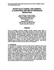
Figure 12: The Knowledge Grid architecture. Figure 12 shows the general architecture of the Knowledge Grid system and its main components. The High-level K-Grid layer includes services used to compose, validate, and execute a distributed knowledge discovery computation. The main services of the High-level K-Grid are: • The Data Access Service (DAS) is responsible for the publication and search of data to be mined (data sources), and the search of discovered models (mining results). • The Tools and Algorithms Access Service (TAAS) is responsible for the publication and search of extraction tools, data mining tools, and visualization tools. • The Execution Plan Management Service (EPMS). An execution plan is represented by a graph describing interactions and data flows between data sources, extraction tools, data mining tools, and visualization tools. The Execution Plan Management Service allows for defining the structure of an application by building the corresponding execution graph and adding a set of constraints about resources. The execution plan generated by this service is referred to as abstract execution plan, because it may include both well identified resources and abstract resources, i.e., resources that are defined through constraints about their features, but are not known a priori by the user. • The Results Presentation Service (RPS) offers facilities for presenting and visualizing the extracted knowledge models (e.g., association rules, clustering models, classifications). The Core K-Grid layer offers basic services for the management of metadata describing the available resources features of hosts, data sources, data mining tools, and visualization tools. This layer coordinates the application execution by attempting to fulfill the application requirements with respect to available Grid resources. The Core K-Grid layer comprises two main services: • The Knowledge Directory Service (KDS) is responsible for handling metadata describing Knowledge Grid resources. Such resources include hosts, data repositories, tools and algorithms used to extract, analyze, and manipulate data, distributed knowledge discovery execution plans, and knowledge models obtained as result of the mining process. The metadata information is represented by XML documents stored in a Knowledge Metadata Repository (KMR). • The Resource Allocation and Execution Management Service (RAEMS) is used to find a suitable mapping between an abstract execution plan and available resources, with the goal of satisfying the constraints (CPU, CoreGRID TR-0046

21

storage, memory, database, network bandwidth) imposed by the execution plan. The output of this process is an instantiated execution plan, which defines the resource requests for each data mining process. Generated execution plans are stored in the Knowledge Execution Plan Repository (KEPR). After the execution plan activation, this service manages the application execution and the storing of results in the Knowledge Base Repository (KBR).

3.2

SOA and the Grid

The Service Oriented Architecture (SOA) is essentially a programming model for building flexible, modular, and interoperable software applications. Concepts behind SOA are not new, they are derived from component based software, the object oriented programming, and some other models. Rather new is, on the contrary, the broad application and acceptance in modern scientific and business oriented networked systems. The increasing complexity in software development, due to its strong relationship with business and scientific dynamicity and growth, requires high flexibility, the possibility to reuse and integrate existing software, and a high degree of modularity. The solution proposed by SOA can enable the assembly of applications through parts regardless of their implementation details, deployment location, and initial objective of their development. Another principle of service oriented architectures is, in fact the reuse of software within different applications and processes. A service is a software building block capable of fulfilling a given task or business function. It does so by adhering to a well defined interface, defining required parameters and the nature of the result (a contract between the client of the service and the service itself). A service, along with its interface, must be defined in the most general way, in the view of its possible utilization in different contexts an for different purposes. Once defined and deployed, services operates independently of the state of any other service defined within the system, that is they are like “black boxes.” External components are not aware of how they perform their function, they care merely that they return the expected result. Nonetheless, services independence does not prohibit to have services cooperating each other to achieve a common goal. The final objective of SOA is just that, to provide for an application architecture within which all functions are defined as independent services with well-defined interfaces, which can be called in defined sequences to form business processes [11]. When designing services it is important to take into proper account the question of granularity, i.e., it is important to understand what is the amount of functionality that a service should provide. In general, a coarse-grained service has more chances to be used by a wide number of applications and in different contexts, while a fine-grained service is targeted to a specific function and is usually more easy to implement. In summary, the service-oriented architecture is both an architecture and a programming model, it allows the design of software that provides services to other applications through published and discoverable interfaces, and where the services can be invoked over a network. When speaking about SOA thoughts go immediately to Web services, but there is a substantial difference between them. Web services are essentially a web-based implementation of SOA, thus they provide for a particular communication framework within which services can be deployed and operated. Actually, Web services are the most popular implementation of SOA, the reasons of this being, basically, that they are based on universally accepted technologies like XML and SOAP. The Web is not the only area that has been attracted by the SOA paradigm. Also the Grid, can provide a framework whereby a great number of services can be dynamically located, relocated, balanced, and managed so that needed applications are always guaranteed to be securely executed, regardless of the load placed on the system and according to the principles of on-demand computing. The trend of the latest years proved that not only the Grid is a fruitful environment for developing SOA-based applications, but also that the challenges and requirement posed by the Grid environment can contribute to further developments and improvements of the SOA model. The Grid community has adopted the Open Grid Services Architecture (OGSA) as an implementation of the SOA model within the Grid context. In OGSA every resource is represented as a Web Service that conforms to a set of conventions and supports standard interfaces. OGSA provides a well-defined set of Web Service interfaces for the development of interoperable Grid systems and applications [20]. Recently the WS-Resource Framework (WSRF) has been adopted as an evolution of early OGSA implementations [16]. WSRF defines a family of technical specifications for accessing and managing stateful resources using Web Services. The composition of a Web Service and a stateful resource is termed as WS-Resource. The possibility to define a “state” associated to a service is the most important difference between WSRF-compliant Web Services, and pre-WSRF ones. This is a key feature in designing Grid applications, since WS-Resources provide a way to represent, advertise, and access properties related to both computational resources and applications. Besides,

CoreGRID TR-0046

22

the WS-Notification specification defines a publish-subscribe notification model for Web Services, which is exploited to notify interested clients and/or services about changes that occur to the status of a WS-Resource. The combination of stateful resources and the notification pattern can be exploited to build distributed, long-lived Grid applications in which the status of the computation is managed across multiple nodes, and services cooperate in a highly-decentralized way.

3.3

Knowledge Grid WSRF services

This section describes the design and implementation of the Knowledge Grid in terms of the OGSA and WSRF models. In this implementation, each Knowledge Grid service (K-Grid service) is exposed as a Web Service that exports one or more operations (OPs), by using the WSRF conventions and mechanisms. The operations exported by High-level K-Grid services (DAS, TAAS, EPMS, and RPS) are designed to be invoked by user-level applications, whereas operations provided by Core K-Grid services (KDS and RAEMS) are thought to be invoked by High-level and Core K-Grid services. Local interaction

OPs

Possibly remote interaction

OPs

DAS

TAAS

Client interface OPs

OPs

EPMS

RPS

Figure 13: Interactions between a user and the Knowledge Grid environment. As shown in Figure 13, a user can access the Knowledge Grid functionalities by using a client interface that is located on her/his machine. The client interface can be an integrated visual environment that allows the user to perform basic tasks (e.g., search of data and software, data transfers, simple job executions), as well as distributed data mining applications described by arbitrarily complex execution plans. The client interface performs its tasks by invoking the appropriate operations provided by the different High-level K-Grid services. Those services are in general executed on a different host; therefore the interactions between the client interface and High-level K-Grid services are possibly remote, as shown in the figure. Figure 14 describes the general invocation mechanisms between clients and K-Grid services. All K-Grid services export three mandatory operations - createResource, subscribe and destroy - and one or more servicespecific operations. The createResource operation is used to create a WS-Resource, which is then used to maintain the state (e.g., results) of the computations performed by the service-specific operations. The subscribe operation is used to subscribe for notifications about computation results. The destroy operation removes a WSResource. The figure shows a generic K-Grid service exporting the mandatory operations and two service-specific operations operationX and operationY. A client interacting with the K-Grid service is also shown. Note that a “client” can be either a client interface or another K-Grid service. Here we assume that the client need to invoke, in sequence, the operations operationX and operationY. In order to do that, the following steps are executed (see Figure 14). 1. The client invokes the createResource operation, which creates a new stateful resource, used to maintain the state of the subsequent operations. The state is expressed as Properties within the resource.

CoreGRID TR-0046

23

K-Grid service 1

createResource 1

2

3

Client

4

subscribe operationX

3 4 6

5

7

6 8

operationY

WS-Resource Properties

8

destroy

Figure 14: General K-Grid service invocation mechanism. 2. The K-Grid service returns the EndpointReference of the created resource. The EndpointReference is unique within the Web Service, and distinguishes this resource from all other resources in that service. Subsequent requests from the client will be directed to the resource identified by that EndpointReference. 3. The client invokes the subscribe operation, which subscribes for notifications about subsequent properties changes. Hereafter, the client will receive notifications containing all the new information (e.g., execution results) that will be stored as resource properties. 4. The client invokes operationX in an asynchronous way. Therefore, the client may proceed its execution without waiting for the completion of the operation. The execution is handled within the WS-Resource created on Step 1, and all the outcomes of the execution are stored as properties. 5. Changes to the WS-Resource Properties are notified directly to the client. This mechanism allows for the asynchronous delivery of the execution results whenever they are generated. 6. The client invokes operationY. As before, the execution is handled within the resource created on Step 1, and results are stored in its properties. 7. The execution results are delivered to the client again through a notification mechanism. 8. The client invokes the destroy operation, which destroys the resource created on Step 1. Table 4 shows the services and the main associated operations of the Knowledge Grid.

4

Conclusions

In the first part of this report we have discussed APStream , a new algorithm for approximate frequent itemset mining on streams. APStream exploits a novel interpolation method to infer the unknown past counts of some itemsets, which are frequents only on recent data. Since the support values computed by the algorithm are approximate, we have also proposed a method for establishing a pair of upper and lower bounds for each interpolated value. These bounds are computed using the knowledge of subpattern frequencies in past data, and of a hash based compressed representation of past data. Experimental tests shows that the solution produced by APStream is a good approximation of the exact global result. The interpolation works particularly well for dense dataset, achieving a similarity close to 100% in the best case. The adaptive behavior of APStream allows us to limit the amount of used memory. The proposed interpolation framework for frequent pattern mining is based on the merge of partial results, using interpolation to replace missing data. The framework was originally proposed for distributed datasets [39], and, in this report, has been extended to stream datasets. Thanks to the generality of the proposed approach, it can be easily extended also to other, more challenging, cases, like Frequent Sequences, Frequent Closed Itemsets, and settings involving multiple distributed streams. CoreGRID TR-0046

24

Table 4: Description of main K-Grid service operations. Service

Operation

Description

DAS

publishData

This operation is invoked by a client for publishing a newly available dataset. The publishing requires a set of information that will be stored as metadata in the local KMR.

DAS

searchData

The search for available data to be used in a KDD computation is accomplished during the application design by invoking this operation. The searching is performed on the basis of appropriate parameters.

TAAS

publishTools

This operation is used to publish metadata about a data mining tool in the local KMR. As a result of the publishing, a new DM service is made available for utilization in KDD computations.

TAAS

searchTools

It is similar to the searchData operation except that it is targeted to data mining tools.

EPMS

submitKApplication

This operation receives a conceptual model of the application to be executed. The EPMS generates a corresponding abstract execution plan and submits it to the RAEMS for its execution.

RPS

getResults

Retrieves results of a performed KDD computation and presents them to the user.

KDS

publishResource

This is the basic, core-level operation for publishing data or tools. It is thus invoked by the DAS or TAAS services for performing their own specific operations.

KDS

searchResource

The core-level operation for searching data or tools.

RAEMS

manageKExecution

This operation receives an abstract execution plan of the application. The RAEMS generates an instantiated execution plan and manages its execution.

In the second part of this report we have addressed the problem of defining and composing Grid services for implementing distributed knowledge discovery and data mining services on SOA-Grids. We have discussed some Grid-based data mining systems, described the Knowledge Grid system, and presented Grid services for searching Grid resources, composing software and data elements, and manage the execution of the resulting data mining application on a Grid. In particular, we have described the definition of data mining Grid services in the context of the Knowledge Grid architecture. Services and their associated operation presented allow for data and tools publication and searching, submission application models for execution, management of the mapping of an application on Grid resources/services for execution and retrieving the results produced by a data mining application.

References [1] Workshop on frequent itemset mining implementations FIMI’03 in conjunction with ICDM’03. fimi.cs.helsinki.fi, 2003.

In

[2] R. Agarwal, C. Aggarwal, and V. V. V. Prasad. A tree projection algorithm for generation of frequent itemsets. Parallel and Distributed Computing, 2000. [3] R. Agrawal, T. Imielinski, and A. Swami. Mining association rules between sets of items in large databases. In Proceedings of the 1993 ACM SIGMOD International Conference on Management of Data, pages 207–216, Washington, D.C., 1993. [4] R. Agrawal and J.C. Shafer. Parallel mining of association rules. In IEEE Transaction On Knowledge and Data Engineering, 1996. [5] R. Agrawal and R. Srikant. Fast algorithms for mining association rules. In Proc. 20th Int. Conf. Very Large Data Bases, VLDB, pages 487–499. Morgan Kaufmann, 1994. [6] Brian Babcock, Shivnath Babu, Mayur Datar, Rajeev Motwani, and Jennifer Widom. Models and issues in data stream systems. In Proceedings of the twenty-first ACM SIGMOD-SIGACT-SIGART symposium on Principles of database systems, pages 1–16. ACM Press, 2002. [7] F. Berman. From teragrid to knowledge grid. Communitations of the ACM, 44(11):27–28, 2001. CoreGRID TR-0046

25

[8] M. Cannataro, D. Talia, and P. Trunfio. Knowledge grid: High performance knowledge discovery services on the grid. In Proc. of the 2nd Int. Workshop on Grid Computing (Grid 2001), 2001. [9] Mario Cannataro and Domenico Talia. The knowledge grid. Communitations of the ACM, 46(1):89–93, 2003. [10] Joong Hyuk Chang and Won Suk Lee. Finding recent frequent itemsets adaptively over online data streams. In KDD ’03: Proceedings of the ninth ACM SIGKDD international conference on Knowledge discovery and data mining, pages 487–492, New York, NY, USA, 2003. ACM Press. [11] K. Channabasavaiah, K. Holley, and E.M. Tuggle. Migrating to a service-oriented architecture, 2003. http://www-106.ibm.com/developerworks/library/ws-migratesoa. [12] M. Charikar, K. Chen, and M. Farach-Colton. Finding frequent items in data streams. In ICALP ’02: Proceedings of the 29th International Colloquium on Automata, Languages and Programming, pages 693–703, London, UK,, 2002. Springer-Verlag. [13] Cheung, Han, Ng, Fu, and Fu. A fast distributed algorithm for mining association rules. In PDIS: International Conference on Parallel and Distributed Information Systems. IEEE Computer Society Technical Committee on Data Engineering, and ACM SIGMOD, 1996. [14] G. Cormode and S. Muthukrishnan. What’s hot and what’s not: tracking most frequent items dynamically. In PODS ’03: Proceedings of the twenty-second ACM SIGMOD-SIGACT-SIGART symposium on Principles of database systems, pages 296–306. ACM Press, 2003. [15] G. Cormode and S. Muthukrishnan. An improved data stream summary: the count-min sketch and its applications. J. Algorithms, 55(1):58–75, 2005. The ws-resource framework [16] K. Czajkowski et al. 106.ibm.com/developerworks/library/ws-resource/ws-wsrf.pdf.

version

1.0,

2004.

http://www-

[17] E.D. Demaine, A. L´opez-Ortiz, and J.I. Munro. Frequency estimation of internet packet streams with limited space. In ESA ’02: Proceedings of the 10th Annual European Symposium on Algorithms, pages 348–360, London, UK,, 2002. Springer-Verlag. [18] C. Domingo, R. Gavalda, and O. Watanabe. Adaptive sampling methods for scaling up knowledge discovery algorithms. Data Mining and Knowledge Discovery, 6(2), 2002. [19] U. M. Fayyad, G. Piatetsky-Shapiro, P. Smyth, and R. Uthurusamy, editors. Advances in Knowledge Discovery and Data Mining. AAAI Press, 1998. [20] I. Foster, C. Kesselman, J. Nick, and S. Tuecke. The Physiology of the Grid, volume Grid Computing: Making the Global Infrastructure a Reality, pages 217–249. Wiley, 2003. [21] V. Ganti, J. Gehrke, and R. Ramakrishnan. Mining Very Large Databases. IEEE Computer, 32(8):38–45, 1999. [22] C. Giannella, J. Han, J. Pei, X. Yan, and P.S. Yu. Mining Frequent Patterns in Data Streams at Multiple Time Granularities. AAAI/MIT Press, 2003. [23] E-H.S. Han, G. Karypis, and V. Kumar. Scalable parallel data mining for association rules. In IEEE Transaction on Knowledge and Data Engineering, 2000. [24] J. Han, J. Pei, and Y. Yin. Mining frequent patterns without candidate generation. In Proc. of the ACM SIGMOD Int. Conference on Management of Data, 2000. [25] J.D. Holt and S.M. Chung. Mining association rules using inverted hashing and pruning. Inf. Process. Lett., 83(4):211–220, 2002. [26] R. Jin and G. G. Agrawal. An algorithm for in-core frequent itemset mining on streaming data. IEEE ICDM’05, 2005. [27] H. Kargupta and P. Chan. Advances in Distributed and Parallel Knowledge Discovery. AAAI Press, 2000. CoreGRID TR-0046

26

[28] Richard M. Karp, Scott Shenker, and Christos H. Papadimitriou. A simple algorithm for finding frequent elements in streams and bags. ACM Trans. Database Syst., 28(1):51–55, 2003. [29] G. Manku and R. Motwani. Approximate frequency counts over data streams. In In Proceedings of the 28th International Conference on Very Large Data Bases, August 2002. [30] Misra.J. and D. Gries. Finding repeated elements. Technical report, Ithaca, NY, USA,, 1982. [31] A. Mueller. Fast sequential and parallel algorithms for association rules mining: A comparison. Technical Report CS-TR-3515, Univ. of Maryland, 1995. [32] S. Orlando, P. Palmerini, R. Perego, and F. Silvestri. Adaptive and resource-aware mining of frequent sets. In Proc. of the 2002 IEEE International Conference on Data Mining, ICDM, 2002. [33] S. Orlando, R. Perego, and C. Silvestri. A new algorithm for gap constrained sequence mining. To appear in Proceedings of ACM Symposim on Applied Computing SAC - Data Mining track, Nicosia, Cyprus, March 2004. [34] J.S. Park, M.S. Chen, and P.S. Yu. An Effective Hash Based Algorithm for Mining Association Rules. In Proceedings of 1995 ACM SIGMOD Int. Conf. on Management of Data, pages 175–186. [35] S. Parthasarathy. Efficient progressive sampling for association rules. In Proceedings of the 2002 IEEE International Conference on Data Mining (ICDM’02), page 354. IEEE Computer Society, 2002. [36] A. Savasere, E. Omiecinski, and S.B. Navathe. An efficient algorithm for mining association rules in large databases. In VLDB’95, Proceedings of 21th International Conference on Very Large Data Bases, pages 432– 444. Morgan Kaufmann, September 1995. [37] T. Scheffer and S. Wrobel. Finding the most interesting patterns in a database quickly by using sequential sampling. Journal of Machine Learning Research, 3, 2003. [38] A. Schuster and R. Wolff. Communication Efficient Distributed Mining of Association Rules. In ACM SIGMOD, Santa Barbara, CA, April 2001. [39] C. Silvestri and S. Orlando. Distributed approximate mining of frequent patterns. In Proceedings of ACM Symposim on Applied Computing SAC - Data Mining track, March 2005,. [40] Hannu Toivonen. Sampling large databases for association rules. In T. M. Vijayaraman, Alejandro P. Buchmann, C. Mohan, and Nandlal L. Sarda, editors, In Proc. 1996 Int. Conf. Very Large Data Bases, pages 134–145. Morgan Kaufman, 09 1996. [41] R. Wolff and A. Schuster. Mining Association Rules in Peer-to-Peer Systems. In The Third IEEE International Conference on Data Mining (ICDM’03), Melbourne, FL, November 2003. [42] M.J. Zaki. Parallel and distributed association mining: A survey. In IEEE Concurrency, 1999. [43] M.J. Zaki. Scalable algorithms for association mining. IEEE Transactions on Knowledge and Data Engineering, 12:372–390, May/June 2000.

CoreGRID TR-0046

27