list-based online mining algorithm for discovering frequent sensor value sets. Through extensive experiments, we compare the performance of ILB against an ...
HKU CS Tech Report TR-2005-02
Online Algorithms for Mining Inter-Stream Associations From Large Sensor Networks K. K. Loo
Ivy Tong
Ben Kao
David Cheung
Department of Computer Science, The University of Hong Kong, Hong Kong. {kkloo|smtong|kao|dcheung}@cs.hku.hk
Abstract. We study the problem of mining frequent value sets from a large sensor network. We discuss how sensor stream data could be represented that facilitates efficient online mining and propose the interval-list representation. Based on Lossy Counting, we propose ILB, an intervallist-based online mining algorithm for discovering frequent sensor value sets. Through extensive experiments, we compare the performance of ILB against an application of Lossy Counting (LC) using a weighted transformation method. Results show that ILB outperforms LC significantly for large sensor networks.
1
Introduction
Data mining is an area of active database research because of its applicability in various areas such as decision support and direct marketing. One of the important tasks of data mining is to extract frequently occurring patterns or associations hidden in very large datasets. Different off-line data mining algorithms have been devised for mining data of different nature. As a couple of examples, there are the classic Apriori algorithm for market-basket transactions [1] and SPADE for mining sequence data [21]. There are also algorithms for mining text, time series, multimedia objects, and DNA sequences [4, 13, 14, 20]. In recent years, stream processing and in particular sensor networks has attracted much research interest [5, 17]. Stream processing poses challenging research problems due to large volumes of data involved and, in many cases, on-line processing requirements. As an example application, a telecommunication network monitoring system installs network sensors that report link bandwidth utilizations [8]. The data is used for detecting congestion, balancing load, and signaling alarms when abnormal conditions arise. Discovering association between sensor values is very important in this application. For example, if one finds that the loads of several links that are connected to the same switch are often high at the same time and cause congestion, the network engineers could consider installing additional switches or selectively re-routing the traffic to achieve better load balancing. As another example, enforcing network security often requires continuous monitoring of network traffic, such as the number of packets received and sent,
and the number of DNS lookup requests. Such statistics can be modeled as sensors that report continuously the corresponding figures. To detect attacks, one needs to distinguish “typical” and “atypical” system behaviors. For example, if the outbound traffic of a subnet is significantly larger than its inbound traffic while the reverse is the norm, the network administrator should be alerted. The examples given above share a number of common properties: – The number of sensors is huge. – Each sensor derives a continuous rapid update stream of values. – Due to the large volume of data, it is important that only “interesting” knowledge be extracted to aid decision making. – Discovering associations among values from different sensor streams is desirable. – Since many applications, such as monitoring systems, are reactive in nature, data analysis algorithms are preferably online. – Due to large data volumes, algorithms are preferably one-pass. That is, multiple scans over the dataset should be avoided. With the above observation, we study in this paper the problem of mining frequently occurring sensor values that co-exist temporally from large-scaled sensor networks. We argue that existing data mining algorithms are inadequate in a large sensor network environment. We discuss how existing solutions could be adapted to such an environment and propose an interval-list-based algorithm that takes advantage of the special characteristics of sensor data to achieve better performance. 1.1
Data Model, Representation, and Frequent Value Sets
Any device that detects and reports the state of a monitored attribute can be regarded as a sensor. For example, thermometer, barometer and anemometer are sensors for monitoring weather conditions, while a stock quotation system is a system of sensors for monitoring stock prices. In our model, we assume that a sensor only takes on a finite number of discrete states. (For continuous values, we assume that a suitable quantization method is applied.) Also, we assume that a sensor only reports state changes. (An alternative model would require a sensor to report its state periodically even when there are no state changes. This model could be mapped to ours by simply removing duplicate state values.) A sensor stream can thus be considered as a sequence of updates (or values) such that each update is associated with a time at which the state change occurs. To illustrate, Figure 1 shows a system of six binary sensors (S1 , ..., S6 ), each could be in one of two possible states, namely “low” (L) or “high” (H). The figure indicates, for example, that S1 ’s state is H from time 0 to time 15. Our goal is to discover associations among sensor values that co-exist during a significant portion of time. For example, from Figure 1, we see that sensors S2 and S3 are both “high” during the time interval [6,10], or four seconds. Since our example has a 15 seconds span, the set of sensor values, namely, {S2 = H, S3 =
S
H 1 |
S2
L |
S3
L |
S4
H |
S5
L |
S6
H | 0
L | H |
L |
H |
L |
L |
H | H |
Table 1. A simple transformation
L |
L | 1
2
H | 3
Transaction ID S1 S2 S3 S4 S5 S6 1 H L L H L H 2 H L L H L H 3 H L L H L L 4 H L L L L L 5 H L L L L L 6 H L H L L L
4
5
6
7
8
9
10 11 12 13 14 15
- time/s
Transaction ID S1 S2 S3 S4 1 H L L H 2 H L L H 3 H L L L 4 H L H L
S5 L L L L
S6 weight H 2 L 1 L 2 L 1
Fig. 1. Sensor data Table 2. A weighted transformation
H}, co-exist for a fraction of 4/15 of time. We use the term support to refer to the fraction of time during which a set of sensor values co-exist in the stream data. We call a sensor value set frequent if its support exceeds a user-specified support threshold ρs . Our association analysis is about finding frequent sensor value sets from a large set of rapidly updating sensor streams. If one considers a sensor value, such as “S1 = H”, as an item, mining frequent value sets is similar to mining frequent itemsets. One possible approach is to transform the stream data into a dataset of transactions, and then apply a traditional mining algorithm like Apriori to the resulting dataset. A straightforward data transformation would quantize time into regular intervals, or clock ticks. A transaction (or itemset) is then derived for each clock tick by taking a snapshot of the sensor states. Using our example in Figure 1, if each clock tick lasts one second, Table 1 shows the first few transactions derived. The simple transformation suffers from the difficulty of determining a suitable clock tick. To cover all state changes, it is obvious that a clock tick has to be shorter than the time between any two updates from any sensors. For example, in Figure 1, an update of sensor S3 at time 5 is followed by an update of S2 at time 6. So, a clock tick cannot last more than one second. On the other hand, if a small clock tick is chosen, the derived dataset is huge with many duplicated transactions. For example, from Table 1, we see that transactions 4 and 5 are the same. For a large sensor network with rapidly updating streams, the derived dataset could be too big to allow efficient processing. To reduce the size of the dataset, we could derive a transaction only when there is an update (from any sensor). With this approach, different snapshots of the sensor states could have different life-span. Each transaction is thus augmented with a weight that equals the life-span of the snapshot from which the transaction is derived. Table 2 illustrates this transformation. Typically, algorithms for mining frequent itemsets determine the support of an itemset, say X, by counting the number of transactions that contain X. With the weighted transformation, those algorithms have to be modified so that the weights of transactions are taken into account during support counting.
Another problem with the weighted transformation approach is that the dataset is still very large with a lot of redundancy. One can observe from Table 2 that successive transactions only differ by one sensor value. This redundancy causes traditional mining algorithms to perform poorly for three reasons. First, the large dataset makes scanning the dataset an expensive operation. Second, for a sensor network that consists of n sensors, each transaction could contain n items. Hence, for large sensor networks, transactions are large. While a market basket transaction may contain a few dozens items, a transaction derived from a large sensor network could contain a few thousand items. Large transactions may pose problems to existing mining algorithms. Third, subset testing, which is done frequently by many mining algorithms for determining whether an itemset is contained in a transaction, is redundantly performed. Due to the high similarity between two successive transactions, most subsets contained by one are also contained by another. A more efficient algorithm should strive for avoiding redundant computation. A third transformation that could avoid the redundancy problem is to represent a sensor stream by an interval list. Given a sensor S and a value v, the interval list IL(S = v) is a list of (start-time, end-time) pairs. Each pair specifies the start time and the end time of a time interval during which S assumes the value v. Using Figure 1 as an example again, the interval list of S3 = L is IL(S3 = L) = {(0, 5), (10, 15)}. With the interval list representation, the support of a sensor value, S = v, is simply the total length of all the intervals in IL(S = v) expressed as a fraction of the length of the stream history. We can extend the definition of interval list to cover sensor value set as well. For example, the interval list of the value set X = {S3 = L, S6 = H} is IL(X) = {(0, 2), (13, 15)}). Given a value set A = A1 ∪ A2 , one can easily see that the interval list IL(A) is equal to the intersection of IL(A1 ) and IL(A2 ). Intuitively, the interval-list representation has the potential of supporting a more efficient mining algorithm in a large sensor network environment over the traditional apriori-based approaches. This is because the representation avoids data redundancy which leads to a much smaller dataset. Moreover, determining the support of a sensor value set is achieved by list intersection. This avoids the large number of redundant subset testing performed by apriori-based algorithms. As we have argued, due to the reactive nature of monitoring systems and the large volume of data generated by a massive sensor network, data analysis algorithms should be online and one-pass. Most traditional mining algorithms, however, are off-line and that they require multiple scanning of the dataset. If a system had an unlimited amount of memory, counting itemsets’ (or sensor value sets in our context) supports can be done in one pass by storing (and tallying) a count for every itemset that has ever appeared in the stream. For large sensor networks, this approach is obviously infeasible due to the large number of counts the algorithm has to keep track of. In [19] Manku and Motwani proposed the Lossy Counting algorithm, which is an online, one-pass procedure for finding frequently occurring itemsets from a data stream of transactions. The algorithm is an approximation algorithm with
an accuracy guarantee. Given a user-specified support threshold ρs and an error bound parameter ǫ, Lossy Counting reports a set of itemsets L with the following properties: (1) all itemsets with supports exceeding ρs are in L, and (2) L does not contain any itemset whose support is smaller than ρs − ǫ. That is to say, even if Lossy Counting reports an itemset X that is not frequent, X’s support is guaranteed to be not too far off the support threshold. In this paper we study how the Lossy Counting framework can be used to derive online one-pass algorithms for mining large sensor streams under the two data representations (weighted transactions and interval list). The rest of the paper is structured as follows. We formally define the problem of finding frequently co-existing sensor value sets in Section 2. In Section 3, we review the Lossy Counting algorithm. In Section 4, we define interval list and propose an interval-list-based algorithm for solving the problem. We compare the interval-list-based algorithm against Lossy Counting using the weighted representation. Section 5 reports the experimental results. Section 6 reviews some related research work, and finally, Section 7 concludes the paper.
2
Problem definition
We define a sensor as a device for monitoring and reporting the states of some physical attribute. The set of all possible states of a sensor S is called the domain of S. We assume that every sensor has a finite domain. (If a sensor’s state is taken from a continuous domain, we assume an appropriate quantization method is applied that maps the domain into a finite one.) We assume that the state of a sensor changes at discrete time instants called updates. The state of a sensor stays the same between updates. A sensor value is a state reported by a sensor. We denote a sensor value by S = v where S is a sensor and v is the state reported. If the state of sensor S is v at a certain time t, we say that the sensor value S = v is valid at time t. Given a time interval I, if S = v is valid at every instant of I, we say that S = v is valid in I. A sensor network consists of a number of sensors. A set of sensor values V is valid in an interval I if all sensor values in V are valid in I. We call such a set a valid value set in I. We assume that all sensors in a sensor network start reporting values at time 0. At any time instant T (> 0), the support duration of a value set V, denoted by SD(V), is the total length of all non-overlapping intervals within [0, T ] in which V is valid. We define the support of V, denoted by sup(V), as SD(V)/T , that is, it measures the fraction of time in [0, T ] during which the value set V is valid. Given a user specified support threshold ρs , a value set V is frequent if sup(V) ≥ ρs . As we have mentioned in the introduction, we are interested in deriving an online one-pass algorithm for finding the set of frequent value sets. Unfortunately, such an algorithm would require keeping track of all possible value sets that have ever occurred in the data stream and tallying their support durations. The high memory and processing requirements render this approach infeasible. As an
N1
�
N2
-
Transaction number
-
D1 Current batch of D2 transactions B
T1
� D1
(a) A stream of transactions
T2
Current batch of updates B
Time
-
D2
(b) Streams of sensor updates
Fig. 2. Lossy Counting
alternative, we adopt the Lossy Counting framework proposed in [19]: instead of finding the exact set of frequent value sets, we report all value sets that are frequent plus some value sets whose supports are guaranteed to be not less than ρs − ǫ for some user-specified error bound ǫ.
3
Lossy Counting
In [19], Manku and Motwani propose Lossy Counting, a simple but effective algorithm for counting approximately the set of frequent itemsets from a stream of transactions. Since our algorithms use the framework of Lossy Counting , we briefly describe the algorithm in this section. With Lossy Counting, a user specifies a support threshold ρs and an error bound ǫ. Itemsets’ support counts are stored in a data structure D. We can consider D as a table of entries of the form (e, f, ∆), where e is an itemset, f is an approximate support count of e, and ∆ is an error bound of the count. The structure D is properly maintained such that if N is the total number of transactions the system has processed, the structure D satisfies the following properties: P1: If the entry (e, f, ∆) is in D, then f ≤ fe ≤ f + ∆, where fe is the exact support count of e in the N transactions. P2: If the entry (e, f, ∆) is not in D, then fe must be less than ǫN . We describe how D is maintained incrementally so that the above properties hold. The data structure D is initially empty. To update D, transactions are divided into batches. The size of a batch is limited by the amount of memory available. The data structure D is updated after a batch of transactions is processed. Figure 2(a) illustrates the update procedure of D. Let B be a batch of transactions. Let N1 denote the number of transactions before B and let D1 denote the data structure D before B is processed. Let us assume that D1 is properly maintained (i.e., D1 satisfies Properties P1 and P2). When the batch B is processed, Lossy Counting enumerates itemsets that are present in B and count their supports in B. Let e be an itemset that appears in B whose support count w.r.t. B is fB . The data structure D is then updated by the following simple rules (D2 denotes the updated D in the figure): Insert: If D1 does not contain an entry for e, the entry (e, fB , ǫN1 ) is created in D unless fB + ǫN1 ≤ ǫN2 , where N2 is the total number of transactions processed including those in B.
Update: Otherwise, the frequency f of e in D1 is incremented by fB . Delete: After all the updates are done, an entry (e, f, ∆) in D is deleted if f + ∆ ≤ ǫN2 . At any point in time, if a user requests the set of itemsets with supports larger than ρs , Lossy Counting reports each itemset e such that there is an entry (e, f, ∆) in D and that f ≥ (ρs − ǫ)N , where N is the number of transactions processed so far. It is proved in [19] that the exact support of any so reported itemset e must exceed ρs − ǫ and that all frequent itemsets (i.e., those with supports exceeding ρs ) are reported. For an efficient implementation of Lossy Counting, certain optimization is done. For example, a special BUFFER structure is used to represent the transactions in a batch and a special SETGEN module is used to selectively enumerate itemsets in a batch and to count their supports. To apply Lossy Counting to our frequent value set mining problem, A few modifications have to be made. These changes are illustrated in Figure 2(b). First, we have to transform our sensor updates into a stream of transactions. This can be done using either the simple transformation (see Table 1) or the weighted transformation (see Table 2). These transactions are again partitioned into batches. Second, N1 and N2 , which are the number of transactions processed before and after a batch B (see Figure 2(a)) are replaced by T1 and T2 , which are the lengths of the stream history just before and just after B. Third, we consider a sensor value (such as S = v) as an item and we consider a sensor value set as an itemset. Finally, frequency counts should now be interpreted as support durations, that is the amount of time during which a particular value set is valid. These mappings should be applied when executing the three rules for updating the data structure D. For example, the insert rule now reads: Insert: If D1 does not contain an entry for a value set V, the entry (V, fB , ǫT1 ) is created in D if fB + ǫT1 > ǫT2 , where fB is the support duration of V in B. As we have discussed, since the simple transformation suffers from the difficulty of choosing an appropriate clock tick and from the problem of space efficiency, the weighted transformation is more desirable. As a result, transaction weights should be taken into account when Lossy Counting “counts” the support durations of value sets that are present in batch B for updating the structure D. In particular, the Buffer and SetGen modules of Lossy Counting have to be modified. The modified code is shown in the Appendix.
4
Interval List
Another way of representing sensor stream data is to use interval lists. In this section we formally define interval lists and discuss how they could be used to mine frequent value sets under the Lossy Counting framework. An interval is a continuous period of time. We denote an interval I by (t, t¯), where t and t¯ are the start time and the end time of the interval, respectively. The duration of I is given by δ(I) = t¯ − t. Given two intervals I1 = (t1 , t¯1 ) and I2 = (t2 , t¯2 ) such that t1 ≤ t2 , if t2 < t¯1 , the two intervals are said to be
1 2 3 4 5 6 7 8 9 10 11 12 13
C1 ← set of all size-1 value sets; B ← {IL(V) | V ∈ C1 }; i ← 1; While Ci 6= ∅ do Foreach V ∈ TCi do IL(V) = {IL(v) | v ∈ V}; SD = δ(IL(V)); Update(D, V, SD, T1 , T2 , ǫ); end-for Di ← {(V, f, ∆) | (V, f, ∆) ∈ D ∧ |V| = i}; Ci+1 ← ApGen(Di , i + 1); i ← i + 1; end-while
Fig. 3. Procedure for updating D using the interval list representation.
1 function Update (D, V, SD, T1 , T2 , ǫ) 2 if (∃(V, f, ∆) ∈ D) do 3 f ← f + SD; 4 if (f + ∆ < ǫT2 ) do 5 remove all entries (X, ., .) from D where X ⊇ V; 6 end-if 7 else if (SD ≥ ǫ(T2 − T1 )) do 8 D = D ∪ (V, SD, ǫT1 ); 9 end-if
Fig. 4. Function Update()
overlapping. The intersection of two overlapping intervals I1 and I2 is given by I1 ∩ I2 = (t2 , min(t¯1 , t¯2 )). An interval list is a sequence of non-overlapping intervals. The intervals in an interval list are ordered P by their start time. The duration of an interval list IL is given by δ(IL) = δ(I) | I ∈ IL. Given S two interval lists IL1 and IL2 , their intersection is defined as: IL1 ∩ IL2 = {I1 ∩ I2 | I1 ∈ IL1 ∧ I2 ∈ IL2 }. Given a set of sensor value V, we use the notation IL(V) to denote the interval list that contains all and only those intervals in which the value set V is valid. We call such an interval list the interval list of V. Given two sensor value sets, V1 and V2 , it can be easily verified that the interval list of V1 ∪V2 can be obtained by intersecting the interval lists of V1 and V2 . That is, IL(V1 ∪V2 ) = IL(V1 )∩IL(V2 ). The interval list representation can be used to mine frequent value sets under the Lossy Counting framework in the following way. First of all, time is partitioned into a number of intervals, each corresponds to a batch of sensor updates (see Figure 2(b)). Instead of representing a batch of updates as a set of weighted transactions, the updates are represented by the interval lists of the sensor values. Similar to the case of Lossy Counting, the size of a batch is limited by the amount of buffer memory available. Also, a data structure D is again used that keeps track of certain sensor value sets’ support durations. The function and properties of D is the same as those described in Section 3. In Lossy Counting (with the modification listed in the Appendix applied for handling weighted transactions), sensor value sets are enumerated by the SETGEN module that also counts the value sets’ support durations within a batch. These counts are used to update the data structure D at the end of processing a batch. If the batch of sensor updates is represented by interval lists instead of weighted transactions, an alternative way of enumerating and counting sensor value sets for updating D is required. Here, we describe such a procedure. Our procedure follows the iterative strategy of Apriori and is outlined in Figure 3. The number of sensor values in a value set V is its size. The procedure starts by collecting all size-1 value sets into a set of candidates, C1 . The batch B is represented by a set of interval lists, one for each sensor value. The procedure then executes a while loop. During each iteration, a set of candidate value sets, Ci , is considered. Essentially, each value set V in Ci is of size i and that V has the
potential of being included in D after the update. In other words, V’s support duration up to time T2 has the potential of exceeding ǫT2 . The procedure then verifies whether V should be included in D by finding its support duration in batch B. This is achieved by first computing IL(V), the interval list of V in batch B, through intersecting the interval lists of relevant sensor values, followed by determining the total length of all the intervals in IL(V). The support duration is stored in a temporary variable SD. The structure D is then updated by function Update() (to be discussed shortly). After all candidates in Ci are processed, all the entries in D for size-i value sets are properly updated. These entries are collected in Di . The set Di is used to generate the candidate set Ci+1 for the next iteration. More specifically, a size-(i + 1) value set V is put into Ci+1 unless there is a size-i subset V ′ of V that is not in Di . This is because by Property P2 of D (see Section 3), if the entry (V ′ , f, ∆) is not in Di , we know that the support duration of V ′ w.r.t. time T2 must be smaller than ǫT2 . Since the support duration of V cannot be larger than the support duration of its subset V ′ , the support duration of V is smaller than ǫT2 as well. That is, V should be left out of D and needs not be considered. Given a value set V and its support duration in a batch B, updating D essentially follows the three update rules listed in Section 3. Figure 4 shows the function Update(). There are a number of optimizations that can be applied to speed up our procedure of processing a batch. For example, in Figure 3, Line 6, the interval list of a value set V is computed by intersecting the interval lists of all the values in V. For example, if V = {S1 = v1 , S2 = v2 , S3 = v3 }, IL(V) is obtained by intersecting IL(S1 = v1 ), IL(S2 = v2 ) and IL(S3 = v3 ). Note that for V to be included in C3 , we require that all size-2 subsets of V are in D2 . That is to say, we would have already determined, for example, IL({S1 = v1 , S2 = v2 }) and IL({S2 = v2 , S3 = v3 }) in the previous iteration. Since IL(V) = IL({S1 = v1 , S2 = v2 }) ∩ IL({S2 = v2 , S3 = v3 }), if we had retained the interval lists of the size-2 value sets, determining IL(V) only require the intersection of two interval lists instead of three. Retaining all intermediate interval lists, however, requires a lot of space, especially when there are many value sets in D. An alternative approach would be to temporarily retain a small number of intermediate interval lists that are likely be used shortly after they are generated. For example, suppose one sorts the value sets in Ci in such a way that successive value sets considered in the forloop (Figure 3, Line 8) share many common values, then only a few intermediate interval lists need to be kept. Specifically, after a value set V is processed in the for-loop, we retain all the interval lists of V’s subsets; other interval lists are discarded. If the next value set, say Y, shares many common elements with V, then the intermediate interval list IL(V ∩ Y) can be re-used since IL(Y) = T IL(V ∩ Y) ∩ ( IL(v) | v ∈ Y − V). Our interval-list-based algorithm for mining frequent value sets uses this optimization.
600 500 400 300 200 100 0 0
100
200 300 400 No. of sensors
500
600
Fig. 5. Dataset size under two representations
5
ILB LC
2500 Time taken in seconds
Size of data representation in MB
ILB LC
700
2000 1500 1000 500 0 0.05
0.10 0.15 Support threshold
0.20
Fig. 6. Running time vs. ρs (600-sensor network)
Results
We perform extensive experiments comparing the performance of the mining algorithms using different data representations. The experiments are performed on a 4-CPU Pentium III Xeon 700MHz machine running SunOS 5.8. In this section we summarize some representative results. We use LC to denote the Lossy Counting algorithm using the weighted transformation described in Section 3 with all the necessary modifications applied (including those mentioned in the Appendix). We use ILB to denote the Interval-List-Based Lossy Counting algorithm described in Section 4. To evaluate the algorithms’ performance and to understand their characteristics, we constructed a synthetic data generator that generates sensor stream updates. The generator is a very flexible one in that it allows us to simulate many different aspects of a sensor stream system. The details of the data generator is documented in Appendix B. As we have alluded to earlier, one major advantage of the interval list representation is that it is more space-efficient than the weighted representation. Figure 5 shows the size of the dataset generated for a stream history of 92000 time units when the number of sensors in the network varies from 100 to 600. In the experiment, the update rates of all the streams are the same. Since the amount of memory required to represent a stream’s updates under the interval list approach is proportional to the number of updates in the stream, the dataset size grows linearly w.r.t. the number of sensors under ILB. The weighted transformation representation, however, does not scale well. This is because, as the number of sensor streams increases, not only does the number of sensor updates (and thus the number of transactions) increase, the size of each transaction also increases proportionally. This results in a quadratic growth of the dataset size under LC. The dataset size has a significant impact on the algorithms’ performance. As an example, Figure 6 shows the execution times of LC and ILB under different support threshold ρs for a 600-sensor network. From the figure, we see that both algorithms take more time to finish when ρs decreases. This is because a smaller support threshold means more and larger
frequent value sets. This leads to more support duration counting and for the case of ILB, more iterations. For this large sensor network, Figure 6 shows that ILB is much more efficient than LC. The performance gain is particularly impressive when ρs is small. To understand the performance difference, let us consider the adverse factors that affect the two algorithms’ performance. For ILB, a source of inefficiency comes from the repeated interval list intersections performed in computing the interval lists of candidate value sets (see Figure 3, Line 6). Even with the optimization we mentioned in Section 4 applied, some redundant list intersections are inevitable. For example, when ILB computes the interval list of the candidate value set {S1 = v1 , S2 = v2 , S3 = v3 }, the intersection of IL(S1 = v1 ) and IL(S2 = v2 ) would be computed even though IL({S1 = v1 , S2 = v2 }) should have already been computed in the previous iteration when the candidate value set {S1 = v1 , S2 = v2 } is considered. A smaller ρs implies larger and more candidates and thus the effect of redundant list intersection is more substantial, causing ILB to take more time. For LC, a major source of inefficiency comes from the large amount of memory required to represent the dataset. Recall that transactions are processed in batches. The number of sensor updates contained in a batch is limited by the amount of buffer memory available. From Figure 5, we see that for a 600-sensor network, the dataset size under LC is 31 times larger than that under ILB. In other words, for LC, a batch contains 31 times fewer updates than that of ILB. The small batch size causes the phenomenon of false alarm to happen in LC. To understand false alarm, let us consider a value set V whose support in the stream history is less than ǫ. Referring to Figure 2(b), which illustrates the processing of a batch B, LC has to update the data structure D from D1 to D2 based on the support duration of the value sets in B. Recall that the purpose of D is to keep track of all value sets whose maximum supports (considering both the known durations and the maximum error bounds) exceeds ǫ. Ideally, the value set V should be kept out of D for its insufficient support. Now, consider the (modified) insert rule (second last paragraph, Section 4), V is inserted into D if fB > ǫ(T2 − T1 ), where fB is V’s support duration in B. If the batch size is small, ǫ(T2 − T1 ) is small. So, even if the support of V < ǫ over the whole stream history, the occurrences of V may be concentrated locally in the batch B for it to just exceed the small threshold ǫ(T2 − T1 ). If so, V is inserted in D. However, due to its small support over the whole stream history, V will get kicked out of D eventually, perhaps when the next batch of updates is considered. This argument suggests that with a small batch size, the structure D is likely to contain many value sets unnecessarily. This significantly slows down LC due to many unnecessary update operations applied to D. To illustrate the effect of false alarm, Table 3 shows the maximum number of entries D ever reaches under ILB and LC for two particular sets of experiment settings. From the table, we see that D contains many more entries under LC than under ILB, signifying that false alarm is much more severe under LC. In
ILB LC
ρs ǫ ILB LC 5% 0.5% 40,895 19,966,164 8% 0.8% 14,059 70,969 Table 3. Maximum size of D
Time taken in seconds
2000 1500 1000 500 0 0.00
0.02
0.04 0.06 0.08 Support threshold
0.10
Fig. 7. Running time vs. ρs (400-sensor network)
fact, when ρs = 5%, there are simply too many false alarms for LC to complete execution within a reasonable amount of time. Figure 7 compares the performance of ILB and LC for a (smaller) 400-sensor network. From the figure, we see that the performance difference between ILB and LC is not as drastic as in the 600-sensor case. However, ILB still outperforms LC by a significant margin. For a 400-sensor network, the dataset size is much smaller for LC (see Figure 5). This allows a larger batch and thus the effect of false alarm is ameliorated.
6
Related Work
Data stream analysis has recently attracted much attention in the research community. In particular, data stream modeling and query processing are discussed in [2, 11, 3]. Besides, there are studies on solving traditional data mining problems, such as classification [9, 15], clustering [12] and frequent pattern mining [19, 7, 16, 6, 10], in stream environments. Click stream analysis is an example application of stream data classification problems [9]. The goal of the application is to predict from web request data the web sites that users in an organization frequently access. The prediction is useful for caching purposes. In [9], a novel decision tree-based algorithm, the Hoeffding tree, is devised for this problem. The Hoeffding tree incrementally updates a decision tree by using only a small sample of the dataset but with good accuracy. The algorithm is extended in [15] to handle time-changing streams. Stanford’s STREAM project has studied approximate k-median clustering with guaranteed probabilistic bound [12]. The techniques can be used in network intrusion detection to find any bursts of activities or abrupt changes in real time. Frequent pattern mining is an important problem in applications such data mining and computer network monitoring. In Section 3, we reviewed the Lossy Counting algorithm which generates frequent itemsets with supports accurate to within a user-specified error bound. Besides, algorithms are proposed for various applications such as finding large flows in network traffic [10], solving the top k (iceberg) queries [7, 16] and estimating the most frequent items in a data stream using very limited storage space [6]. All these applications require identification of frequent patterns in a data stream.
Sensor network is one of the emerging applications of data streams. Among recent research works in this area, a framework for building an efficient data stream management system for sensor networks is presented in [17] and the problem of query processing in sensor networks is addressed in [18].
7
Conclusion
In this paper we study the problem of mining frequent sensor value sets from a massive sensor network. We discuss a few methods for representing sensor stream data. These include mapping sensor streams into transactions using either the simple transformation or the weighted transformation, and the interval-list approach. We discuss the pros and cons of the representations and derive online mining algorithms, namely, LC and ILB, for the two approaches. We evaluate the algorithms’ performance through experiments. Due to space limitation, only the performance results from a couple of experiment settings are presented. The results show that ILB could outperform LC by a significant margin, particularly for large sensor networks. Besides the two illustrative examples shown in Section 5, we have compared the two algorithms under various experiment settings and have observed similar performance behavior. The interval list representation is thus a viable option in representing a massive sensor network.
References 1. Rakesh Agrawal and Ramakrishnan Srikant. Fast algorithms for mining association rules in large databases. In VLDB, pages 487–499, 1994. 2. Brian Babcock, Shivnath Babu, Mayur Datar, Rajeev Motwani, and Jennifer Widom. Models and issues in data stream systems. In PODS, pages 1–16, 2002. 3. Shivnath Babu and Jennifer Widom. Continuous queries over data streams. ACM SIGMOD Record, 30(3):109–200, September 2001. 4. Sergey Brin, Rajeev Motwani, and Craig Silverstein. Beyond market baskets: Generalizing association rules to correlations. In SIGMOD Conference, 1997. 5. Donald Carney and et al. Monitoring streams - a new class of data management applications. In VLDB, pages 215–226, 2002. 6. Moses Charikar, Kevin Chen, and Martin Farach-Colton. Finding frequent items in data streams. In ICALP, pages 693–703, 2002. 7. Erik D. Demaine, Alejandro L´ opez-Ortiz, and J. Ian Munro. Frequency estimation of internet packet streams with limited space. In ESA, pages 348–360, 2002. 8. Alin Dobra and et al. Processing complex aggregate queries over data streams. In SIGMOD Conference, pages 61–72, 2002. 9. Pedro Domingos and Geoff Hulten. Mining high-speed data streams. In KDD, pages 71–80, 2000. 10. Cristian Estan and George Varghese. New directions in traffic measurement and accounting. In SIGCOMM, pages 323–336, 2002. 11. Johannes Gehrke, Flip Korn, and Divesh Srivastava. On computing correlated aggregates over continual data streams. In SIGMOD Conference, 2001. 12. Sudipto Guha, Nina Mishra, Rajeev Motwani, and Liadan O’Callaghan. Clustering data streams. In FOCS, pages 359–366, 2000.
13. Jiawei Han, Guozhu Dong, and Yiwen Yin. Efficient mining of partial periodic patterns in time series database. In ICDE, pages 106–115, 1999. 14. Jiawei Han and et al. DNA-Miner: A system prototype for mining DNA sequences. In SIGMOD Conference, 2001. 15. Geoff Hulten, Laurie Spencer, and Pedro Domingos. Mining time-changing data streams. In KDD, pages 97–106, 2001. 16. Richard M. Karp and et al. A simple algorithm for finding frequent elements in streams and bags. ACM Trans. Database Syst., 28(1):51–55, 2003. 17. Samuel Madden and Michael J. Franklin. Fjording the stream: An architecture for queries over streaming sensor data. In ICDE, pages 555–566, 2002. 18. Samuel Madden, Michael J. Franklin, Joseph M. Hellerstein, and Wei Hong. TAG: A Tiny AGgregation service for ad-hoc sensor networks. In OSDI, 2002. 19. Gurmeet Singh Manku and Rajeev Motwani. Approximate frequency counts over data streams. In VLDB, pages 346–357, 2002. 20. Osmar R. Za¨ıane and et al. MultiMediaMiner: A system prototype for multimedia data mining. In SIGMOD Conference, pages 581–583, 1998. 21. Mohammed Javeed Zaki. SPADE: An efficient algorithm for mining frequent sequences. Machine Learning, 42(1/2):31–60, 2001.
Item-ids
a b d e a c d b c d
Trans. boundary 0 0 0 1 0 0 1 0 0 1
Fig. 8. The Buffer structure
A
Modifying Lossy Counting for weighted transactions
We mentioned in Section 3 that we need to modify Lossy Counting so that the algorithm can handle weighted transactions. In this appendix, we give an account on As a recapitulation, Lossy Counting is an online algorithm for finding frequent itemsets with approximate support counts from a stream of market-basket transaction data. The algorithm guarantees three things: (1) all frequent itemsets are reported, (2) the reported support of any itemset is at most ρs + ǫ, and (3) the actual support of any reported itemset is at least ρs − ǫ, where ǫ is some user-specified error tolerance. A conceptual description on how Lossy Counting works is given in Section 3. In [19], an efficient implementation was proposed with the following characteristics. – The data structures used in the implementation are highly compact. – For finding itemset supports, a depth-first approach is adopted. – No candidate generation is needed when finding itemset supports. A.1
Efficient implementation of Lossy Counting
The proposed implementation includes three modules, namely, Buffer, Trie and SetGen. In particular, Buffer is a structure for keeping incoming data as a batch of transactions in the available memory. Trie maintains the data structure D described in Section 3. Finally, SetGen generates itemsets with supports in the current batch of transactions. Since modifications are made only to Buffer and SetGen, we focus our discussion on these two modules. For a full description on the proposed implementation, please refer to [19]. Buffer The Buffer structure contains two parts: an array for storing the transactions and a bitmap for marking boundaries of transactions. As transactions, which are in the form of sets of item-ids, are being read into memory, they are laid out one after another in a big array. Here, we assume that a lexicographical order exists among item-ids and that transactions are sorted by that order. An auxiliary bitmap is used to mark the boundary of transactions. Each bit in the bitmap corresponds to an element in the array. A “True” (1) in the bitmap means that the corresponding element in the array is the end of some transaction.
Memory address 0 1 2 3 4 5 6 7 8 9 a b d e a c d b c d Item-ids Trans. boundary 0 0 0 1 0 0 1 0 0 1 Heap
0 / / / / a b c d e
(a) After inserting abde into Heap Memory address 0 1 2 3 4 5 6 7 8 9 a b d e 0 c d b c d Item-ids Trans. boundary 0 0 0 1 0 0 1 0 0 1 Heap
4 / / / / a b c d e (b) After inserting acd into Heap
Fig. 9. Construction of the initial Heap
Suppose transactions abde, acd, bcd are among a batch of transactions read in Buffer. Figure 8 shows an example of the Buffer structure. Transactions are flattened and item-ids are put in the array. A “True” bit in the bitmap marks the end of a transaction. SetGen SetGen uses a priority queue called Heap to support its operations. Intuitively, the Heap is a collection of chains of pointers. A pointer is the memory address of some transaction stored in Buffer. Initially, each chain contains pointers to transactions that start with the same item-id in Buffer. An interesting property of the Heap is that, for the smallest item-id in the Heap that contains a chain, the number of pointers in the chain gives the support count of the item (or itemset as we will see later) in this batch. It is because any transaction in Buffer that contains the smallest item-id must start with the item-id. In addition, each pointer corresponds to a transaction in Buffer and thus contributes one count to the support of the itemset. In practice, the Heap is designed to be as memory-efficient as possible by keeping only the head of the chain for each item-id and converting some of the item-ids in Buffer to pointers to represent the chain. The following paragraphs illustrate how this works. Assume that the array in Figure 8 starts at memory address “0”, and recall that the Buffer in Figure 8 contains three transactions abde, acd, bcd. We construct the initial Heap by inserting memory addresses of the smallest item-id of each transaction into Heap. As an illustration, the first transaction is abde which starts with a at memory address “0”. Then we insert the address “0” to Heap under the chain a. Figure 9(a) shows the Heap after this step.
Memory address 0 1 2 3 4 5 6 7 8 9 a b d e 0 c d b c d Item-ids Trans. boundary 0 0 0 1 0 0 1 0 0 1 Heap
1 5 / / ab ac ad ae
Fig. 10. Generating new heap by extending a
The second transaction, acd, also starts with a, which is located at memory address “4”. Thus, we insert the address “4” into Heap under a. Now, since the chain head is occupied by some memory address, we know that a chain exists under this item-id and so we need to do an insertion to the chain. This is done by converting the a at memory address “4” in Buffer to the original chain head (i.e., address “0”) and make “4” the new head of the chain. See Figure 9(b). When we finish adding all transactions to Heap, we can get all transactions starting with a particular item-id by following memory addresses in Heap and Buffer. For example, to get all transactions starting with a, we consult the Heap and get the chain head “4”. The element at memory address “4” in the Buffer is “0”, so we know that the transaction at “0” also starts with a. We comment that the last transaction of the chain is reached if an item-id instead of an address is encountered. After the Heap is initialized, SetGen generates frequent itemsets starting from the smallest entry that has a chain in Heap. SetGen first checks whether the singleton itemset has enough support to remain in D. If so, SetGen extends the itemset by one item. This is done by recursively generating a new Heap following successors of the pointers in the chain. For example, we have two pointers within the chain a in Figure 9(b). Suppose a remains in D after D is updated with the support count of a in this batch. Then we extend the itemset a by one item and generate a new heap by adding successors of the pointers in the chain a to the new Heap. In other words, if a pointer does not refer to a transaction boundary, the address of the item-id that follows is inserted to the new Heap. Figure 10 shows the new Heap generated by extending the itemset a. When the recursion returns, the chain is removed after successors of the pointers in the chain are added to the Heap. Removal of a chain is done by reverting the corresponding pointers in Buffer to the item-id and set the head of the chain to null in Heap. A.2
Modifying Lossy Counting for weighted transactions
As we have discussed in the previous sub-section, support of an itemset is determined by the number of pointers in a chain. This works fine for market-basket data since every transaction is equally important in terms of support. However, for sensor data, if we adopt the weighted transformation (See Section 1), the
derived transactions can have different weights because snapshots can last for different life-spans. When determining the support of a value set, we need to consider the weights of different transactions. To make Lossy Counting capable of handling weighted transactions, modifications to the Buffer and SetGen modules are necessary. There are two possibilities. – The weight of each transaction is stored in the array in Buffer as if it was an item-id. Then, a True bit in the bitmap indicates that the corresponding element of the array is the weight of some transaction. Each time when SetGen references a transaction, it obtains the weight of the transaction by traversing down the array until it reaches an element which corresponds to a True bit in the bitmap. – The weight of each transaction is stored alongside each pointer in the chain when the initial heap is constructed. As SetGen generates value sets and constructs new Heaps, successor of a pointer is added alongside the weight attached to the pointer to a new Heap. We tried both modifications and we found that the second method outperformed the first one. This is because searching weights in the first modification was slow, especially when transactions are long. Our experimental study (Section 5) uses the second modification.
B
Synthetic data generation
We generated synthetic data to evaluate the performance of interval list-based algorithms. The data model emulates a system of homogeneous sensors, and the data generation process can be divided into three phases. Firstly, we decide the properties, namely, the probabilities of different states and the frequency that the sensor refreshes its value, of each sensor. Then, we generate a set of potentially frequent patterns in a way similar to that described in [1]. Finally, data are generated as state changes “happen” at the sensors under the influence of the potentially frequent patterns. In the rest of this sub-section, we give a detailed description on our data generation model. B.1
Basic settings of the data model
Table 4 lists the parameters of our data model. The model emulates a system of n homogeneous sensors S1 , S2 , ..., Sn , whereas possible states of the sensors are denoted by v1 , v2 , ..., vx . In the first phase of the data generation process, we decide the properties of the sensors. For the sensor Si , let ti denote the mean time that zi refreshes its value and let Pi = (pi,1 , pi,2 , ..., pi,x ), the state probability vector for Si , denote the probabilities of different states. The value ti is obtained from an exponential distribution with mean equals to t. The probabilities are determined as follows.
Symbol Meaning General settings: |D| No. of sensor updates to be generated n No. of sensors x No. of possible states for each sensor p1 , p2 , ..., px Mean probabilities for each of the possible states t Mean time that a sensor refreshes its state Potentially frequent patterns: |F | No. of potentially frequent patterns l Mean length of potentially frequent patterns w Base weight of potentially frequent patterns a Mean no. of effective potentially frequent patterns c Coherence factor Table 4. User input
The j-th value in the vector, i.e., pi,j , is firstly obtained by weighting pj by a normally distributed random number with mean 1 and variance 0.25. Then the probabilities are normalized so that they sum to 1. B.2
Generation of potentially frequent patterns
The second phase, generation of potentially frequent patterns, is inspired by the data model described in [1]. Each potentially frequent pattern is a set of sensor values accompanied by a weight and a corruption level. The weight of a pattern controls the effect of a pattern to the sensors. It is obtained from an exponential distribution with unit mean plus the base weight w, which is a user input. The corruption level, on the other hand, controls the regularity of the data generated, as we will see in the next stage of the data generation process. The corruption level is obtained from a normal distribution with mean 0.5 and variance 0.1. The length (i.e., number of sensor values) of each potentially frequent pattern is obtained from a Poisson distribution with mean l. For the first pattern, distinct sensors are randomly selected. Since, in our experiment settings (Section 5), we are only interested in sensors with “On” state, we set all sensors in the pattern to “On”. For each of the remaining patterns, a fraction of the sensor values is picked from its previous pattern, where the fraction is decided by a an exponential distribution with mean equals to a correlation level, which is set to 0.5. The remaining sensor values are randomly picked in the same way as for the first pattern. B.3
Data generation
At any time, state changes are affected by a pool of effective potentially frequent patterns. The pool is maintained as follows. The size of the pool is decided by a Poisson distribution with mean a. Then, potentially frequent patterns are selected for the pool by a uniform distribution. For each selected pattern, we
Attribute Notation Value Number of sensors n Variable Size of domain 2 Mean probability vector P < 0.99, 0.01 > Mean length of potentially frequent (PF) value sets l 4% × n Mean number of effective PF value sets a 10 Mean time between update t 1 Table 5. Data generation settings
repeatedly drop a sensor value from the pattern as long as a uniformly distributed random variable between 0 and 1 is less than the corruption level of the pattern. Then, the state probability vectors for the sensors covered by the corrupted pattern are recalculated. For example, let a corrupted pattern, whose weight is w, contain the sensor value Si = vj . Then, for Si , the probability of the state vj is multiplied by w whereas the probability of any other state is divided by w. The probabilities are then normalized so that they sum to 1. The pool remains effective for a period of length t × c. After that, the pool is refreshed and all state probabilities are reset to their original values. Data are generated as state changes are simulated at the sensors. For each sensor, the initial state is decided by throwing an x-faced die with each face weighted by its respective probability. Then, the next state change will “happen” after δ, where δ is determined by repeatedly throwing the x-faced die until it gives a different state from the original one. Each time the die is thrown, a value obtained from an exponential distribution with mean t is added to δ. State changes are taken as data generated, and we repeat this process until we get |D| state changes. Table 5 shows some parameters of the generator and their baseline settings.
C
Discussion - adaptation of the algorithm for a sliding window scenario
In some applications, recent data are more important than those that are dated. For example, to detect for network intrusion, one may only need the data generated by a network monitoring system during the past 10 minutes or so. In other words, data older than 10 minutes become obsolete and are not considered when associations are found. This is an example of “sliding window”. A sliding window can be modelled by a buffer that only contains the most recent data. The amount of data a window holds is called the “width”, denoted by w, of the window. In general, the width need not be fixed. To maintain an exact sliding window is not feasible if the width is very big. It is because we need to keep every sensor update happened in the window so that, when data items obsolete, we know what to remove from the window. To ease space requirements, different algorithms for maintaining sliding windows based on sampling and randomization techniques are developed.
We can make simple modifications to our algorithm to find frequent value sets over a sliding window. Here, let us recall the relevant part of the original algorithm first. In our algorithm, we buffer incoming data as a batch B and find supports of value sets in the batch. Then, we merge the supports into a data structure D, which keeps a bounded over-estimate of the actual support for each value set if its actual support can exceed a pre-defined error-tolerance ǫ. Each entry kept in D is in the form (e, f, ∆) where e is a value set, f is the observed frequency since the entry is added to D, and ∆ is the maximum error such that f ≤ fe ≤ f + ∆ where fe is the actual support. The ∆, obtained by ǫT where T is the length of history before this batch, is fixed when the entry first enters D. We need some changes to extend our algorithm to find frequent value sets over a sliding window. First, we restrict the size of a batch to w/n, i.e., 1-n-th of the width of the sliding window. This allows that, after a batch is processed, we keep the frequency counts of value sets for the batch and discard the raw data. When a batch of data obsoletes, we discount the value set frequency counts for the batch from overall counts. The second change is on the entries in D. We change the format of entries in D to a 3-tuple (e, f, F ), where e is a value set, f is the frequency count of e after the entry enters D, and F is a first-in-first-out queue keeping observed frequencies of e in batches of data that are not obsolete. Each element in F is merely a frequency count, where the last element in F is the observed frequency of e in the latest batch of data, the second last element corresponds to the frequency in the previous batch, and so on. Since the size of a batch is w/n, there are at most n elements in F . Note that, in the original algorithm, there is ∆ which gives an over-estimate of the frequency of e missed before the entry enters D. We comment that it is not necessary here because this information can be deduced from F . Let |F | denote the number of elements in F . If |F | = n, it means the whole window is captured by F and so f is the exact frequency of e during the window. Hence there is no need for an over-estimate and ∆ is 0. If |F | < n, then we need to over-estimate the frequency of e for the portion of the window before the entry is inserted to D. In this case, ∆ is determined by | | × w), where ǫ is the error tolerance and n−|F × w gives the portion ǫ × ( n−|F n n of the window which has no frequency information in F . Finally, the insert, update and delete operations of D are modified as follows. Insert: When an entry is inserted to D, we initialize f to fB where fB is the frequency of e in the current batch B. Besides, the queue F is initialized to contain the only element fB . Update: Given fB the frequency of the value set e in the current batch, to update an existing entry (e, f, F ) in D, we first append a new element fB to F and update f to f + fB . Then, we check whether F contains more than n elements. If so, the leading element of F is removed from F and the frequency count the element represents is deducted from f . Delete: After updating, an entry (e, f, F ) is removed from D if f + ∆ < ǫw, | × w). where ∆ = ǫ × ( n−|F n