Journal of Mathematics Research; Vol. 10, No. 2; April 2018 ISSN 1916-9795 E-ISSN 1916-9809 Published by Canadian Center of Science and Education
Algorithms for Asymptotically Exact Minimizations in Karush-Kuhn-Tucker Methods Koudi Jean1 , Guy Degla 1 , Babacar Mbaye Ndiaye2 & Mamadou Kaba Traor´e3 1
Institute of Mathematics and Physical Sciences, University of Abomey Calavi, Porto-Novo, Benin
2
Laboratory of Mathematics of Decision and Numerical Analysis, University of Cheikh Anta Diop, Dakar, Senegal
3
Computer Laboratory, ISIMA (University of Blaise Pascal), Clermont-Ferrand, France
Correspondence: Babacar Mbaye Ndiaye, Laboratory of Mathematics of Decision and Numerical Analysis. University of Cheikh Anta Diop. BP 45087 Dakar-Fann, 10700, Dakar, Senegal. E-mail:
[email protected] Received: January 2, 2018
Accepted: January 22, 2018
doi:10.5539/jmr.v10n2p36
Online Published: February 19, 2018
URL: https://doi.org/10.5539/jmr.v10n2p36
Abstract We provide two new algorithms with applications to asymptotically exact minimizations with inequalities constraints. These results generalize and improve the works of Andreani, Birgin, Martinez and Schuverdt on minimization with equality constraints. Numerical examples show that our proposed analysis gives convergence results. Keywords: nonlinear programming, augmented lagrangian methods, numerical experiments, approximate KKT point 1. Introduction The Kuhn-Tucker condition is often used to obtain important results in economics, especially in decision problems that occur in static situations, for example to show the existence of a balance for a competitive economy, main agents constraints and so on. Kuhn-Tucker conditions for the optimization problem under inequality and equality constraints have a global shape that naturally incorporate the Lagrange multiplier method (introduced by Lagrange in 1788). The application of this method to an optimization problem under constraint leads to the resolution of the Karush, Kuhn and Tucker (KKT) system. Thoughout this work, we consider on Rn (n ∈ N) the ordering relation ≤ defined by: ∀ u ∈ Rn , ∀ l ∈ Rn , u ≤ l ⇐⇒ [u]i ≤ [l]i ∀ i ∈ {1; ...;{n} where [u]i is the ith component of the row u. We also consider [u]i if [u]i ≥ 0 the operator projection P+ : Rn −→ Rn+ by [P+ (u)]i = 0 otherwise We shall study in this work the optimization problem of type (P) : min f (x)
(1)
x∈K
with K =
{
x ∈ Rn ; gi (x) ≤ 0 ∀ i ∈ I = {1, ..., m}
}
(2)
Under Karush-Kuhn-Tucker constraint qualification, when the problem (1) is differentiable (i.e., all the involved functions are differentiable), a first-order condition for a point x∗ to be optimal is that it satisfies the following system: n ∑ ∇ f (x) + λi ∇gi (x) = 0 i=1 λi gi (x) = 0 ∀ i ∈ I (exclusion condition) λi ≥ 0 ∀ i ∈ I
(3)
When the constraints of the problem are equality constraints, the exclusion condition in (3) becomes obvious. So, to find a solution of the problem (1) is to find a point satisfying the system (3) without the exclusion condition. The manual resolution of this system becomes complicated especially when the size of the problem becomes large. In April 1991, Andrew R. C. et al. published two algorithms in (Andrew, R.C. & et al., 1991) for solving KKT systems arising from differentiable optimization problems under equality constraints K defined by: K =
{
} x ∈ Rn ; hi (x) = 0 ∀ i ∈ I; u ≤ x ≤ l , u ∈ Rn and l ∈ Rn 36
(4)
http://jmr.ccsenet.org
Journal of Mathematics Research
Vol. 10, No. 2; 2018
These algorithms are based on the augmented Lagrangian defined by: ∑ ∑ S ii L(x; λ; S ; µ) = f (x) + λi hi (x) + (hi (x))2 2µ i i∈I i∈I
(5)
where µ ∈ Rm + and S is an invertible diagonal matrix such that 0 < S ii . In 2006, Andreani R. et al., in (Andreani, R. & et al., 2006) have taken up these algorithms by posing ρi = penality parameter. Their algorithms are also based on the augmented lagrangian defined by: ∑ 1∑ L(x, λ, ρ) = f (x) + λi gi (x) + ρi [gi (x)]2 2 i∈I i∈I If all the functions of the constraints are differentiable and if the objective function is differentiable, we have: ∑ ∇ x L(x, λ, ρ) = ∇ f (x) + (λi + ρi gi (x))∇i gi (x)
S ii µi
called
(6)
(7)
i∈I
The principle of these algorithms is to find x ∈ K such that ∥PΩ [x − ∇ x L(x, λ, ρ)] − x∥∞ = 0
(8)
−∇ x L(x, λ, ρ) ∈ T Ω0 (x)
(9)
that is to say
Where PΩ is the projection operator on Ω = {x ∈ Rn : lb ≤ x ≤ ub} In our work, we improve these algorithms in order to adapt them to optimization problems under inequality constraints. Our algorithm guarantees constraint qualifications at the end point of sequence generated by each of these algorithms (and satisfaction of exclusion condition). We modify the estimation of Lagrange multipliers and add a new condition for the resolution of a sub-problem in order to determine the approximate solutions xk at each iteration k. We present the foundations of this algorithm including a convergence analysis result. The rest of the paper is organized as follows. In section 2, we review part of literature on KKT algorithm, followed by an analysis of our algorithm and the obtained results in section 3. Finally, we conclude with prospective recommendations in section 4. 2. Some Preliminaries 2.1 Admissible Direction and Tangent Cone Let K be a feasible set of the problem (P) and x0 be an admissible element. • An admissible direction at x0 is any vector tangent to an arc of curve (sufficiently regular) admissible in x0 . In 0 other words, it is any element d such that there exists (xn ) ∈ K N −→ x0 , ϵn −→ 0 and xnϵ−x −→ d. n xn −x0 Let ωn = ϵn , we obtain ωn −→ d and ϵn ωn + x0 ∈ K ∀ n • The set of all admissible directions is called the tangent cone at x0 of K and denote by T K (x0 ) • The polar cone at x0 of K is T K0 (x0 ) = Suppose that
{ } u : ⟨u, d⟩ ≤ 0 ∀ d ∈ T K (x0 )
{ K = x∈X :
gi (x) ≤ 0, ∀i ∈ I
}
• The linear tangent cone at x0 of K denote by T Klin (x0 ) is defined by { } T Klin (x0 ) = d : ∇gi (x) · d ≤ 0, ∀i ∈ I(x0 ) and its linear polar cone at x0 is
∑ λ ∇g (x ) : λ ≥ 0 ∀ i ∈ I(x ) (T Klin )0 (x0 ) = i i 0 i 0 i∈I(x0 )
37
http://jmr.ccsenet.org
Journal of Mathematics Research
Vol. 10, No. 2; 2018
where I(x0 ) = {i ∈ I; gi (x0 ) = 0} It is easy to see that: T K (x0 ) ⊂ T Klin (x0 )
(10)
(T Klin )0 (x0 ) ⊂ T K0 (x0 )
(11)
and
Recall that the constraint K is qualified at xo if T K (x0 ) = T Klin (x0 )
(12)
Among the multitudes sufficient conditions for the qualification of the constraint, we can mention those such as: Slater (1950) and Karlin (1959) constraints: that often apply in nondifferentiable cases for convex problems. AHUCQ Arrow, Hurwicz and Uzawa Constrained qualification. MFCQ Mangasarian and Fromovitz Constrained qualification (Gerd Wachsmuth, 2013): it guarantees the existence of Lagrange multiplier satisfying the system of Karush Kuhn and Tucker at the optimum. LICQ Linearly Independent Constraint Qualification Gerd Wachsmuth, 2013): which is the strongest of all the qualification constraints that apply to differentiable problems; it guarantees the existence and uniqueness of Lagrange multiplier satisfying the system of Karush Kuhn and Tucker at the optimum. (CPLD) Constant Positive Linear Dependence condition (Qi, L. & Wei, Z., 2000); Definition 2.1]: Let A = {a1 , ..., am } and B = {b1 , ..., bq } be families of elements of Rn such that A ∪ B is no empty set. A and B are q said to be positively linearly dependent if there exists α ∈ Rm + and β ∈ R such that (α; β) , (0; 0) and m ∑ i=1
αi ai +
q ∑
β jb j = 0
(13)
j=1
∗ Otherwise, we say that A and B are positively linearly qualification { } independent. We say that x {satisfies }the ∪ { } constraint ∗ ∗ ∗ ∗ (CPLD), if there exists I1 ⊂ I(x ) = i ∈ I; gi (x ) = 0 , J1 ⊂ J such that the familly ∇gi (x ) ∇h j (x ) is posii∈I {1 } ∪ {j∈J1 } ∗ ∗ tively linearly dependent, if there exists a neighborhood V(x ) such that ∀ x ∈ V(x ) the familly ∇gi (x) ∇h j (x) j∈J1 i∈I1 is lineairely dependent.
2.2 KKT Point We say that a feasible point is a Karush-Kuhn-Tucker point of the problem (1) if it checks the system (3) called KarushKuhn-Tucker (KKT) system. A KKT point is not necessarily a minimum point, it is usually a stationary point (minimum, or maximum, or saddle point). The determination of such a point consists in solving the system (3). Our goal is to determine from these algorithms, the points of KKT which allow to have the exact optimum value. But it is sometimes difficult to reach precisely such a point. 2.3 Approximate KKT Point Consider the optimization probem defined by { } (P) : min f (x) where K = x ∈ Rn ; gi (x) ≤ 0 ∀ i ∈ I = {1, ..., m}, h j (x) = 0, ∀ j ∈ {1, · · · , q} x∈K
(14)
and all the functions are differentiable. A feasible point x∗ is said to be approximate KKT point of (P) if there exists a sequence (xk )k ⊂ Rn that converges to x∗ , k q k a sequence (λk )k ⊂ Rm + , a sequence (µ )k ⊂ R and a sequence (ε )k ⊂ R+ converging to zero such that ) { ( ∑ ∑q k k k k ∇ f (xk ) + m i=1 λi ∇gi (x ) + j=1 µ j ∇ j h j (x ) −→ 0 when k −→ ∞ λki (gi (xk ) + εk ) = 0 ∀ i ∈ I et ∀ k Proposition 2.1. (See (Qi, L. & Wei, Z., 2000); Theorem2.7) Let x∗ be an approximate KKT point that satisfies the (CPLD) condition, then x∗ is a KKT point.
38
(15)
http://jmr.ccsenet.org
Journal of Mathematics Research
Vol. 10, No. 2; 2018
2.4 Some Reminders on Optimality Conditions An immediate consequence of the local optimality of x∗ for (1) is ∇ f (x∗ ) · d ≥ 0 ∀ d ∈ T K (x∗ )
(16)
−∇ f (x∗ ) ∈ (T K0 (x∗ ))
(17)
that is to say {
with K = x ∈ X :
}
gi (x) ≤ 0, ∀i ∈ I . According to KKT condition, the relation (17) implies ∑
λi ∇gi (x∗ ) ∈ T K0 (x∗ )
(18)
i∈I
3. Main Results 3.1 Algorithms Let us first recall that any constrained optimization problem whose feasible set is defined by { K = x ∈ Rn , gi (x) ≤ 0 ∀ i ∈ I = 1, 2, ..., m, h j (x) = 0 ∀ j ∈ J = 1, 2, ..., q}
(19)
can be transformed into a problem of the same type as (1) where all the constraints are inequality constraints. This is because each equality constraint can be transformed into double inequalities. That is to say h(x) = 0 ⇐⇒ h(x) ≤ 0 and h(x) ≥ 0 Our algorithms are based on the augmented lagrangian defined by: ∑ 1∑ L(x, λ, µ) = f (x) + λi gi (x) + ρi (gi (x))2 2 i∈I i∈I
(20)
(21)
Like R. Andreani et al. in (Andreani, R. & et al., 2006), We shall compute at each iteration k a point xk such that ∥PΩ [xk − ∇ x L(xk , λk , ρk )] − xk ∥∞ ≤ εk
(22)
where εk is a decreasing sequence converging to zero. The point xk at iteration k for (22) constitutes a non-obvious subproblem to solve in the algorithm. The following proposition allows us to easily construct a sequence of points under certain hypotheses satisfying (22) m Proposition 3.1. Let Ω be a close subset of Rn , λ ∈ Rm + , ρ ∈ R++ and (xk )k be a sequence defined by:
xk+1 = PΩ [xk − hk ∇ x L(xk , λ, ρ)] (23) ∑ where hk is a sequence that converges to zero and hk < +∞. Then the sequence ∥PΩ [xk − ∇ x L(xk , λk , ρk )] − xk ∥∞ k≥0
converge. Proof
To simplify, let us denote ∇ x L(xk , λ, ρ)] = ∇ x L(xk ) By definition xk ∈ Ω for all k. The projection operator is 1-lipschitzian, thus ∥xk − xk+1 ∥
= ∥xk − PΩ [xk − hk ∇ x L(xk )]∥ = ∥PΩ [xk ] − PΩ [xk − hk ∇ x L(xk )]∥ ≤ ∥xk − (xk − hk ∇ x L(xk ))∥ = ∥hk ∇ x L(xk )∥
(24) (25) (26)
Let Uk = PΩ [xk − ∇ x L(xk , λk , ρk )] − xk . Again the 1-Lipschitzness of the projection we have: ∥Uk+1 − Uk ∥
=
∥xk+1 − xk − (PΩ [xk+1 − ∇ x L(xk+1 )] − PΩ [xk − ∇ x L(xk )])∥ ≤ ∥xk − xk+1 ∥ + ∥xk − xk+1 − (∇ x L(xk+1 ) − ∇ x L(xk ))∥ ≤ 2∥xk − xk+1 ∥ + ∥(∇ x L(xk+1 ) − ∇ x L(xk ))∥ 39
(27) (28) (29)
http://jmr.ccsenet.org
Journal of Mathematics Research
Vol. 10, No. 2; 2018
(xk )k being a sequence of descent towards the optimum, there exists M ≥ 0 such that ∥∇ x L(xk )∥ ≤ M and ∥∇ x L(xk+1 ) − ∇ x L(xk )∥ ≤ M∥xk+1 − xk ∥ then ∥Uk+1 − Uk ∥ ≤ (2 + M)hk
(30)
Let p, q ∈ N (suppose that p ≥ q) we have: ∥U p − Uq ∥ ≤
p−q−1 ∑
U p−s − U p−s−1
(31)
s=0
According to (30) we have:
∥U p − Uq ∥
≤
p+1 ∑
(
(2 + M) h s = 2 + M
p+1 )∑
s=q
As hk −→ 0 and
∑
hs
(32)
s=q
hk < +∞, then Uk are Cauchy sequence. Then it converge because Rn is a complete space.
k≥0
The convergence towards zero will be studied in these propositions to follows. As constraints are inequalities, we shall add a new condition defined by: ∑ | [λk ]i gi (xk ) | ≤ εk ∀ k
(33)
i∈I
in order to satisfy at the end of each algorithm the exclusion condition in the KKT system. This condition will serve to converge rapidly towards the optimum. In fact, it is easy to see that ∑
| [λk ]i gi (xk ) | = 0 ⇐⇒ [λk ]i gi (xk ) = 0
∀ i∈I
(34)
i∈I
In 2006, Andreani R. et al., in (Andreani R. & et al., 2006) have defined the projection on Ω = {x ∈ Rn , lb ≤ x ≤ ub}. The projection on this set can give inadmissible points specially when lb and ub are not well defined according to the admissible set (eg when they are away from the permissible assembly). To approximate advantage the projected to the admissible set we shall define the projection on the set Ω(xk ) = {x ∈ Rn , Ax ≤ b, lb ≤ x ≤ ub} were A = ∇g(xk ) and bi = (∇gi (xk ))T · xk − gi (xk ) ∀ i
(35)
Indeed a point x ∈ Rn will be admissible if and only if gi (x) ≤ 0 ∀ i ∈ {1, ..., m}. Since all the functions are differentiable, at the iteration k + 1 knowing that xk is already determined, gi (xk+1 ) − gi (xk ) = ∇gi (xk )(xk+1 − xk ) + ∥xk+1 − xk ∥ε(xk+1 − xk ) were lim ε(xk+1 − xk ) = 0. Thus, approximately we have g(xk+1 ) ≤ 0 ⇐⇒ ∇g(xk )T · xk+1 ≤ ∇g(xk )T · xk − g( xk ). ∥xk+1 −xk ∥→0
At each iteration it is necessary to solve a quadratic problem defined by min ∥u − x∥2 (∇gi (xk ))T x ≤ (∇g(xk ))T · xk − gi (xk ), (Q) : lb ≤ x ≤ ub x ∈ Rn
1≤i≤m
(36)
It is clear that K ⊂ Ω(xk ) ⊂ Ω ∀ k. Then for all y ∈ Ω and x ∈ Ω(xk ), we have d(y, K) ≥ d(x, K). Also in the stopping criterion we shall impose that gi (x) ≤ 0 ∀ i ∈ I We propose the two following algorithms C1 and C2 . Algorithm C1 x0 ∈ K, τ ∈ [0; 1[, γ > 1, ρ0 ∈ Rm ++ such that [ρ0 ]i = ∥ρ0 ∥∞ ∀i ∈ I, (εk )k ⊂ R+ a decreasing sequence converging to 0 and 0 < ε∗ ≪ 1 40
http://jmr.ccsenet.org
Journal of Mathematics Research
Vol. 10, No. 2; 2018
λ0 ∈ Argmax{L(x0 , λ), λ ≥ 0}
(37)
∥PΩ(xk ) [xk − ∇ x L(xk , λk , ρk )] − xk ∥ ≤ ε∗ and gi (xk ) ≤ ε∗ ∀ i ∈ I
(38)
[λk+1 ]i = P+ ([λk ]i + [ρk ]i [g(xk )]i ) ∀ i ∈ I
(39)
Step1 : Evaluate λ0
Step2 : (Estimate multipliers) If
stop Otherwise :
Step3 : (Update the penalty parameters) ρk+1 = ρk if ∥g(xk )∥∞ ≤ εk and ρk+1 = γρk otherwise Step4 : Solving the subproblem: εk+1
∑ |gi (xk )| = min εk ; 1 + [ρ ] |g (x )| k i i k i∈I
We chose xk+1 such that ∥PΩ(xk ) [xk+1 − ∇ x L(xk+1 , λk+1 , ρk+1 )] − xk+1 ∥∞ +
∑
| [λk+1 ]i gi (xk+1 ) | ≤ εk+1
(40)
(41)
i∈I
Step5 : k ←− k + 1 Return to Step2.
Algorithm C2 x0 ∈ K, τ ∈ [0; 1[, γ > 1, ρ0 ∈ Rm ++ (εk )k ⊂ R+ is a decreasing sequence converging to 0 and 0 < ε∗ ≪ 1 Step1 : Evaluate λ0
Step2 : Estimate multipliers If and
λ0 ∈ Argmax{L(x0 , λ), λ ≥ 0}
(42)
∥PΩ(xk ) [xk − ∇ x L(xk , λk , ρk )] − xk ∥ ≤ ε∗
(43)
∥g(xk )∥∞ ≤ ε∗
(44)
stop Otherwise :
[ρk ]i [g(xk )]i ) ∀ i ∥ρk ∥
(45)
Γk = {i ∈ I, |gi (xk )| ≥ τ∥g(xk−1 )∥∞ }
(46)
[λk+1 ]i = P+ ([λk ]i + Step3 : (Update the penalty parameters) We define the set
If Γk = ϕ then ρk+1 = ρk Otherwise [ρk+1 ]i = γ[ρk ]i if i ∈ Γk and [ρk+1 ]i = [ρk ]i if i < Γk 41
http://jmr.ccsenet.org
Journal of Mathematics Research
Vol. 10, No. 2; 2018
Step4 : Solving the subproblem: εk+1
∑ |gi (xk )| = min εk+1 ; 1 + [ρ ] |g (x )| k i i k i∈I
We checks xk+1 such that ∥PΩ(xk ) [xk+1 − ∇ x L(xk+1 , λk+1 , ρk+1 )] − xk+1 ∥∞ +
∑
|[λk+1 ]i gi (xk+1 )| ≤ εk+1
(47)
(48)
i∈I
Step5 : k ←− k + 1 Return to Step2 Recall that the resolution of the sub-problem in each algorithm is based on the proposition (3.1). The point x0 can also be unfeasible point; in this case we project it in the feasible set Ω and obtain an approximate feasible point. 3.2 Theorical Results Note that, at the end of each algorithm, the sequence (xk )k converge or have a subsequence that converges to a point x∗ according to (3.1). According to (Theorem3 (Andreani R. & et al., 2006)), Andreani et al. (2006) have proved that if x∗ is feasible and satisfies the CPLD constraint qualification then it is an approximate KKT point. Through the following propositions we will give other conditions under which x∗ will be a KKT point Proposition 3.2. Assume that the sequence (xk )k is generated by algorithm C1 and that x∗ is a limit point. Then ∑ (−gi (x∗ )) · ∇gi (x∗ ) ∈ T Ω0 (x∗ )
(49)
i∈I
and if x∗ is feasible, then there exists λi ≥ 0 ∀ i, such that ∑ ∗ 0 λi · ∇gi (x∗ ) ∈ T Ω(x ∗ ) (x )
(50)
i∈I(x∗ )
Proof Remark that ∥PΩ (u + tv) − u∥∞ ≤ ∥PΩ (u + v) − u∥∞ ∀ t ∈ [0; 1] and ∀ u, v ∈ Rn
(51)
Let ρk = ∥ρk ∥∞ ∀ k By Step3 , if the sequence (ρk )k is bounded then there exists k0 such that for all k ≥ k0 , ∥g(xk )∥ ≤ εk which makes it possible to conclude that the limit x∗ is feasible. Otherwise, ρk −→ ∞ and: [
PΩ(xk )
(
∑( ) ] ) [λk ]i + ρk gi (xk ) ∇gi (xk ) − xk xk − ∇ x L(xk , λk , ρk ) − xk = PΩ(xk ) xk − ∇ f (xk ) +
(52)
i∈I
Let u = xk , t =
1 ρk ,
∑ ([λk ]i + ρk gi (xk ))∇gi (xk ) we have and v = − ∇ f (xk ) + i∈I
( )
∇ f (xk ) ∑ [λk ]i
PΩ(xk ) xk − + + gi (xk ) ∇gi (xk ) − xk
≤
PΩ(xk ) (xk − ∇ x L(xk , λk , ρk )) − xk
∞ (53) ρk ρk
i∈I ∞
Hence, for k sufficiently large, we have ρk −→ ∞ and
PΩ(xk ) (xk − ∇ x L(xk , λk , ρk )) − xk
∞ −→ 0 (according to (48)). Then
∗ ∑ ∗ ∗ ∗
PΩ(x∗ ) x − gi (x ) · ∇gi (x ) − x
= 0
i∈I ∞
42
(54)
http://jmr.ccsenet.org
So
∑(
Journal of Mathematics Research
Vol. 10, No. 2; 2018
) 0 ∗ − gi (x∗ ) · ∇gi (x∗ ) ∈ T Ω(x ∗ ) (x )
(55)
i∈I
⟨ ∑ ⟩ ∀ v ∈ T Ω(x∗ ) (x∗ ); v; (−gi (x∗ )) · ∇gi (x∗ ) ≤ 0
(56)
i∈I
If x∗ is feasible, then −gi (x∗ ) ≥ 0 ∀ i, that is, we can conclude that there exists λi ≥ 0 ∀ i such that ∑ 0 ∗ λi · ∇gi (x∗ ) ∈ T Ω(x ∗ ) (x )
(57)
i∈I(x∗ )
Remark 3.1. . ∑ ∑ ∗ ∗ ∗ gi (x∗ )∇gi (x∗ ) = 0, because: gi (x )∇gi (x ) ∈ Ω, we have When x − i∈I
i∈I
∗ ∑ ∗ ∑ ∗ ∗ ∗ ∗ ∗ x = PΩ(x∗ ) x − gi (x )∇gi (x ) = x − gi (x )∇gi (x ) . i∈I
i∈I
In this case we have the following proposition: Proposition 3.3. Assume that the sequence (xk )k is generated by algorithm C2 and that x∗ is a limit point. If there exists k0 such that Γk is an empty set ∀ k ≥ k0 , then x∗ is a feasible point. Proof By S tep3 in algorithm C2 , we have: ∥g(xk0 +1 )∥ < τ∥g(xk0 )∥
(58)
∥g(xk0 +2 )∥ < τ∥g(xk0 +1 )∥ < τ2 ∥g(xk0 )∥
(59) (60)
. . .
(61) (62) (63)
∥g(xk0 +m )∥ < τm ∥g(xk0 )∥
(64)
When m −→ +∞, we have ∥g(x∗ )∥ = 0 , because 0 ≤ τ < 1 . Then g(x∗ ) = 0, that is to say x∗ is feasible and all constraints are active at x∗ . Note that in the case where the number of constraints is high, it is almost impossible to have all the constraints to be active at a point. Proposition 3.4. Assume that the sequence (xk )k is generated by algorithm C2 and that x∗ is a limit point. Then either x∗ is feasible, or there exists ω ∈ Rm ++ such that ∑ 0 ∗ ωi (−gi (x∗ )) · ∇gi (x∗ ) ∈ T Ω(x (65) ∗ ) (x ) i∈I
And if x∗ is feasible, then there exists λi ≥ 0 ∀ i such that ∑ 0 ∗ λi · ∇gi (x∗ ) ∈ T Ω(x ∗ ) (x )
(66)
i∈I(x∗ )
Proof By the proposition (3.3), if there exists k0 such that Γk = ϕ, ∀ k ≥ k0 , then x∗ feasible and g(x∗ ) = 0. Otherwise, ∥ρk ∥ → ∞ By S tep4 we have ∥PΩ [xk+1 − ∇ x L(xk+1 , λk+1 , ρk+1 )] − xk+1 ∥∞ ≤ εk+1 43
(67)
http://jmr.ccsenet.org
Journal of Mathematics Research
which means that [PΩ(xk ) (xk − (∇ f (xk ) +
Vol. 10, No. 2; 2018
∑ ([λk ]i + [ρk ]i gi (xk ))∇gi (xk ))) − xk ] ≤ εk
(68)
i∈I
Hence by relation (51) we obtain
( )
∇ f (xk ) ∑ [λk ]i [ρk ]i [ ]
PΩ xk − + + gi (xk ) ∇gi (xk ) − xk
≤
PΩ(xk ) xk − ∇ x L(xk , λk , ρk ) − xk
∞ ≤ εk ∥ρk ∥ ∥ρk ∥ ∥ρk ∥
i∈I ∞ ( ∇ f (x ) ) ( [λ ] ) ( [ρ ] ) As k → +∞, we have ∥ρk ∥k → 0, ∥ρkk ∥i → 0 and ∥ρkk ∥i → ω∗i and so: k k k
∑
∗ ∗ ∗ ∗ ∗
PΩ(x∗ ) x − ωi gi (x )∇gi (x ) − x
= 0
i∈I
(69)
(70)
Thus ∑ ∑ ∗ ∗ ∗ ∗ ∗ ∗ ∗ ∗ 0 ∗ − ωi gi (x )∇gi (x ) = x − ωi gi (x )∇gi (x ) − x ∈ T Ω(x ∗ ) (x ), that is to say i∈I
i∈I
∑ ∗ 0 ∗ ωi (−gi (x∗ )) · ∇gi (x∗ ) ∈ T Ω(x ∗ ) (x )
(71)
i∈I
Hence if x∗ is feasible −gi (x∗ ) ≥ 0 ∀ i, then there exists λi ≥ 0 ∀ i such that ∑ ∗ 0 λi · ∇gi (x∗ ) ∈ T Ω(x ∗ ) (x )
(72)
i∈I(x∗ )
Note that the results of propositions (3.2) and (3.4) are an implication of the optimality condition defined in. Thus, they do not allow us to assert the optimality of the limit given by each algorithm. The following theorem 3.1 will give us a sufficient condition for the limit to be an optimal point. We note that the convergence towards an admissible point of the algorithms depends on the convergence of the penalty parameters. Theorem 3.1. (Convergence to an optimal point) Assume that the sequence (xk )k is generated by algorithm C1 or C2 and that a limit point x∗ is a feasible point. Then ∗ m ∗ ∗ ∗ ∗ there exists λ∗ ∈ Rm + and ρ ∈ R++ such that ∇ x L(x , λ , ρ ) = 0. That is to say x is an optimal point and the associated ∗ Lagrange multiplicateur is λ . Proof Let us recall that at each iteration k, the set Ω(xk ) being a closed convex set, the projection probem 1 ∥v − (xk − ∇ x L(xk , λk , ρk ))∥22 v∈Ω(xk ) 2 min
(73)
l n has unique solution vk = PΩ(xk ) [xk − ∇ x L(xk , λk , ρk )]. Apply the KKT conditions to (73), there exists e λk ∈ Rm + , µk ∈ R+ and µuk ∈ Rn+ such that: m n n ∑ ∑ ∑ u e v − x + ∇ L(x , λ , ρ ) + [ λ ] ∇g (x ) + [µ ] e − [µlk ] j e j = 0 k k x k k k k i i k k j j i=1 j=1 j=1 (74) [ ] e [ λ ] · ∇g (x ) · v − ∇g (x ) · x + g (x ) = 0 ∀ i k i i k k i k k i k [µu ] ([x ] − u ) = [µl ] (l − [x ] ) = 0 ∀ j k i j k j k j k j j
By S tep4 ∥vk − xk ∥ = ∥PΩ(xk ) [xk − ∇ x L(xk , λk , ρk )] − xk ∥ ≤ εk which implies lim ∥vk − xk ∥ = 0
(75)
k→∞
Hence by (74) xk − vk
=
∇ x L(xk , λk , ρk ) +
m n n ∑ ∑ ∑ [e λk ]i ∇gi (xk ) + [µuk ] j e j − [µlk ] j e j i=1
=
∇ x L(xk , λk , ρk ) +
j=1
n n ∑ ∑ [µuk ] j e j − [µlk ] j e j j=1
j=1
44
(76)
j=1
(77)
http://jmr.ccsenet.org
Journal of Mathematics Research
were λk = λk + e λk Hence, according to (75) we have
Vol. 10, No. 2; 2018
∑ ∑ [ ] lim ∇ x L(xk , λk , ρk ) + [µuk ]i ei − [µlk ]i ei = 0
k→∞
(78)
Let us denote Ω = {x ∈ Rn , lb ≤ x ≤ ub} it is necessary to choose lb and ub such that K ⊂ int(Ω) where int(Ω) denote the interior of Ω . Since xk −→ x∗ and ∥vk − xk ∥ = ∥PΩ(xk ) [xk − ∇ x L(xk , λk , ρk )] − xk ∥ −→ 0 then vk −→ x∗ ∈ int(Ω). Then there exists N ∈ N such that ∀ k ≥ N, lb < vk < ub. According to the exclusion condition in the system (74), [µuk ] j = [µlk ] j = 0 ∀ j. Hence [ ] lim ∇ x L(xk , λk , ρk ) = 0 (79) k→∞
There exists
λ∗
∈
Rm +
∗
and ρ ∈
Rm ++
such that ∇ x L(x∗ , λ∗ , ρ∗ ) = 0
(80)
Then x∗ is an optimal point and the Lagrange multiplicateur associated is λ∗ . Consequence 3.1. (Convergence to an optimal point) Assume that the sequence (xk )k is generated by algorithm C2 and that a limit point x∗ and that there exists k0 ≥ 0 such that ∀ k ≥ k0 , Γk is empty set. Then x∗ is a KKT point. Proof According to the proposition (3.3), x∗ is feasible and g(x∗ ) = 0. Apply the proposition (3.1) we have λ∗ ∈ Rm + and such that ρ∗ ∈ Rm ++ ∑ ∇ x L(x∗ , λ∗ , ρ∗ ) = ∇ f (x∗ ) + ([λ∗ ]i + [ρ∗ ]i gi (x∗ )) · ∇gi (x∗ ) (81) i∈I
=
∑ ∑ ∇ f (x ) + [λ∗ ]i · ∇gi (x∗ ) + [ρ∗ ]i gi (x∗ ) · ∇gi (x∗ ) ∗
i∈I
=
∇ f (x∗ ) +
∑ [λ∗ ]i · ∇gi (x∗ )
(82)
i∈I
(83)
i∈I
According to (80), we can conclude tha x∗ is a KKT point and the Lagrange multiplicateur associat is λ∗ . Consequence 3.2. (Convergence to KKT point) Assume that the sequence (xk ) is generated by algorithm C1 or C2 and that a limit point x∗ is feasible and the familly {∇g( x∗ )}i∈I(x∗ ) is positively linearly dependent with the coeficient αi = −ρ∗i gi (x∗ ) ∀ i ∈ I r I(x∗ ). Then x∗ is KKT point. Proof It is easy to se that ∇ x L(x∗ , λ∗ , ρ∗ ) =
∇ f (x∗ ) +
∑ ([λ∗ ]i + [ρ∗ ]i gi (x∗ )) · ∇gi (x∗ )
(84)
i∈I
=
∇ f (x∗ ) +
∑ ∑ [λ∗ ]i · ∇gi (x∗ ) + [ρ∗ ]i gi (x∗ ) · ∇gi (x∗ ) i∈I
= =
∀ i ∈ I r I(x∗ ), −gi (x∗ ) > 0, as
∑
∇ f (x∗ ) + ∇ f (x∗ ) +
(85)
i∈I
∑ ∑ [λ∗ ]i · ∇gi (x∗ ) + [ρ∗ ]i gi (x∗ ) · ∇gi (x∗ ) i∈I
i∈IrI(x∗ )
i∈I
i∈IrI(x∗ )
∑ ∑ [λ∗ ]i · ∇gi (x∗ ) − [ρ∗ ]i (−gi (x∗ )) · ∇gi (x∗ )
(86) (87) (88)
[ρ∗ ]i (−gi (x∗ )) · ∇gi (x∗ ) = 0 because {∇g( x∗ )}i∈I(x∗ ) is positively lineairely dependent
i∈IrI(x∗ ) ∗
with the coeficient αi = −ρ∗i gi (x ) ∀ i ∈ I r I(x∗ ), we have ∑ ∇ f (x∗ ) + [λ∗ ]i · ∇gi (x∗ ) = ∇ x L(x∗ , λ∗ , ρ∗ ) = 0 i∈I
Then x∗ is a KKT point. 45
(89)
http://jmr.ccsenet.org
Journal of Mathematics Research
Vol. 10, No. 2; 2018
3.3 Numerical Tests We applied these algorithms to solve several problems of references (Hock, W. & Schittkowski, K., 1981; Asaadi, J., 1973; Miele, A. & et al., 1972; Miele, A. & et al., 1972; Biggs, M. C., 1971; Bracken J., 1976; Klaus, S., 2009), and results are presented in the following tables. For simulations, essentially with the algorithm C2 , let τ = 10−5 , γ = 10, εopt = 10−8 and ε f es = 10−8 . The numerical tests were performed by using the software Python (Python Software Foundation) on a computer: 5Intel(R) Core(TM)4 Duo CPU 2.60GHz, 8.0Gb of RAM, under UNIX system. The difference between the two algorithms is in their ways of computations of Lagrange multipliers and penalty parameters. The algorithm C1 is specifically designed to solve the large-scale problems. The Figures 1 2 3 4 5 and 6 (at the end of the tables) represent the evolution of the optimal value as well as the norm of the lagrangian gradient. The behavior of the curves demonstrates the rapid convergence of the algorithm towards the optimum point. However, in the case of problem 5, although the exact solution has been obtained, the curves show us an insufficiency in the convergence that we must solve for the continuation of our work in this direction. We define by: NIter: Number of iterations, MaxIter: Maximal number of iterations, Nv: Number of variable, Nc: Number of constraints, f(x): Objective function, Sol.Alg: the solution found by our algorithm, Sol.ex: Solution found by the source.
Table 1. Results of Problem 1 Problem Classification Source Nv Nc f(x) Constraints Start point Stop criterions NIter/MaxIter Sol.Alg Sol.ex
1 PRB-TP37 Hock W. (Hock, W. & Schittkowski, K., 1981) n=3 m=2 −x1 · x2 · x3 x + 2x2 + 3x3 − 72 ≤ 0 1 −x1 − 2x2 − 3x3 ≤ 0 0 ≤ x ≤ 42 ∀ i = 1, 2, 3 x0 = (10, 10, 10) ∥xk+1 − xk ∥ ≤ εopt or ∥ f (xk+1 ) − f (xk )∥ ≤ εopt 141/1000 (23.99999993, 12.00000002, 12.00000002) (feasible) (24, 12, 12)
Table 2. Results of Problem 2 Problem Classification Source: Nv Nc f(x) Constraints Start point Stop criterions NIter/MaxIter Sol.Alg Sol.ex
2 PRB-T1-3 Asaadi, J.(Asaadi, J., 1973) n=2 m=2 1 3 {3 (x1 + 1) + x2 ) 1 − x1 ≤ 0 −x2 ≤ 0 x0 = (1.125, 0.125) ∥xk+1 − xk ∥ ≤ εopt or ∥ f (xk+1 ) − f (xk )∥ ≤ εopt 4/1000 (1.00000000e + 00, 1.10201928e − 08) (feasible) (1, 0)
46
http://jmr.ccsenet.org
Journal of Mathematics Research
Table 3. Results of Problem 3 Problem Classification Source Nv Nc f(x) Constraints Start point Stop criterions NIter/MaxIter Sol.Alg Sol.ex
3 GPR-T1-1 Miele et al.(Miele, A. & et al., 1972; Coggins, G. M. & et al, 1972) n=2 m=1 log(x12 + 1) − x2 (x12 + 1)2 + x22 − 4 = 0 x0 = (2, 2) ∥xk+1 − xk ∥ ≤ εopt or ∥ f (xk+1 ) − f (xk )∥ ≤ εopt 8/1000 (2.23896809e − 09, 1.73205081e + 00) (feasible) √ (0, 3) (feasible)
Table 4. Results of Problem 4 Problem Classification Source Nv Nc f(x) Constraints Start point Stop criterions NIter/MaxIter Sol.Alg Sol.ex
4 GLR-T1-1 Miele et al.(Miele, A. & et al., 1972) n=2 m=1 1π 2π sin( x12 ) · cos( x12 ) 4x1 − 3x2 ≤ 0 x0 = (0, 0) ∥xk+1 − xk ∥ ≤ εopt or ∥ f (xk+1 ) − f (xk )∥ ≤ εopt 34/1000 (−2.99998922, −3.99998563) (feasible) (−3, −4)
47
Vol. 10, No. 2; 2018
http://jmr.ccsenet.org
Journal of Mathematics Research
Vol. 10, No. 2; 2018
Table 5. Results of Problem 5 Problem Classification Source Nv Nc f(x) Constraints Start point Stop criterions NIter/MaxIter Sol.Alg Sol.ex
5 (cattel-feed) LGI-P1-1 Biggs(Biggs, M. C., 1971), Bracken, McCormick(Bracken J. & McCormick, G. P., 1976) & Schittkowski K. PRB-73(Klaus, S., 2009) n=4 m=3 24.55x1 + 26.75x2 + 39x3 + 40.5x4 x1 + x2 + x3 + x4 − 1 = 0 −2.3x1 − 5.6x2 − 11.1x3 − 1.3x4 + 5 ≤ 0 −12x1 − 11.9x2 − 42.8x3 − 51.4x4 + 21+ 1.645[0.28x2 + 0.19x2 + 20.5x2 + 0.62x2 )] 12 ≤ 0 1 2 3 4 x0 = (1, 1, 1, 1) ∥xk+1 − xk ∥ ≤ εopt or ∥ f (xk+1 ) − f (xk )∥ ≤ εopt 5/1000 (6.42805324e − 01, 1.18335296e − 08, 3.11958636e − 01, 4.52360285e − 02) (feasible) (0.6355216, −0.12e − 11, −0.3127019, 0.05177655) (unfeasible)
Table 6. Results of Problem 6 Problem Classification Source Nv Nc f(x) Constraints Start point Stop criterions NIter/MaxIter Sol.Alg Sol.ex
6 PQR-T1-2 Asaadi J.(Asaadi, J., 1973) n=2 m=2 100(x2 − x12 )2 + (1 − x1 )2 x1 + x22 ≥ 0 x2 + x2 ≥ 0 −2 ≤ x1 ≤ 0.5, x ≤ 1 1 2 x0 = (0, 1) ∥xk+1 − xk ∥ ≤ εopt or ∥ f (xk+1 ) − f (xk )∥ ≤ εopt 11/1000 (0.5, 0.25) (feasible) (0.5, 0.25)
48
http://jmr.ccsenet.org
Journal of Mathematics Research
Table 7. Results of Problem 7 Problem Classification Source Nv Nc f(x)
Constraints
Start point Stop criterions NIter/MaxIter Sol.Alg Sol.ex
7 PQ-T1-1 Liang, J., J., Thomas, P.(Liang, J. J., 1972) n = 13 m= 9 4 13 4 ∑ ∑ ∑ 2 5 xi − 5 xi − xi i=1 i=1 i=5 2x1 + x2 + x10 + x11 − 10 ≤ 0 2x 1 + 2x3 + x10 + x12 − 10 ≤ 0 2x 2 + 2x3 + x11 + x12 − 10 ≤ 0 −8x1 + x10 ≤ 0 −8x 2 + x11 ≤ 0 −8x 3 + x12 ≤ 0 −2x − x5 + x10 ≤ 0 4 −2x − x7 + x11 ≤ 0 6 −2x8 − x9 + x12 ≤ 0 x0 = cos(ones(13)) ∥xk+1 − xk ∥ ≤ εopt or ∥ f (xk+1 ) − f (xk )∥ ≤ εopt 11/1000 (1, 1, 1, 1, 1, 1, 1, 1, 1, 3, 3, 3, 0.99999999) (feasible) (1, 1, 1, 1, 1, 1, 1, 1, 1, 3, 3, 3, 1)
Figure 1. Evolution of the optimal value and the norm of the Lagrangian gradient
49
Vol. 10, No. 2; 2018
http://jmr.ccsenet.org
Journal of Mathematics Research
Figure 2. Evolution of the optimal value and the norm of the Lagrangian gradient
Figure 3. Evolution of the optimal value and the norm of the Lagrangian gradient
50
Vol. 10, No. 2; 2018
http://jmr.ccsenet.org
Journal of Mathematics Research
Figure 4. Evolution of the optimal value and the norm of the Lagrangian gradient
Figure 5. Evolution of the optimal value and the norm of the Lagrangian gradient
51
Vol. 10, No. 2; 2018
http://jmr.ccsenet.org
Journal of Mathematics Research
Figure 6. Evolution of the optimal value and the norm of the Lagrangian gradient
Figure 7. Evolution of the optimal value and the norm of the Lagrangian gradient
52
Vol. 10, No. 2; 2018
http://jmr.ccsenet.org
Journal of Mathematics Research
Vol. 10, No. 2; 2018
4. Conclusion In this work, we proposed an algorithm for solving optimization problems under inequality constraints. We obtained convergence of generated sequence to an optimal solution, satisfying the Karush-Kuhn-Tucker qualification constraints. Simulations on academic data have shown the performance of our method. Indeed, we maded changes in the calculation of the multipliers for searching the point xk+1 when xk is already determined; and defined new set Ω(xk ) associated to each point xk for the projection in order to promote rapid convergence to an feasible point. Acknowledgement The authors thank the anonymous referees for useful comments and suggestions. Gratitute is expressed to the project Centre d’Excellence Africain en Sciences Math´ematiques et Applications (CEA-SMA) for the support of this work. References Andrew, R. C., Nicholas, G., & Phillipe, L. T. (April 1991). A globally convergent augmented lagrangian algorithm for optimization with general constraints and simple bounds. In SIAM J. Numer. Anal. 28(2), 545-572. Andreani, R., Birgin, E. G., Martłnez, J. M., & Schuverdt, M. L. (2006). Augmented Lagrangian methods under the constant positive linear dependence constraint qualification. Math. Program., Ser. B (2008) 111, 5C32. In SpringerVerlag 2006. https://doi.org/10.1007/s10107-006-0077-1 Asaadi, J. (1973). computational comparison of some Nonlinear program. Mathematical programming, 4, 144-154. Biggs, M. C. (1971). computational experience with Murray’s algorithm for constrained minimization, Technical Report, 23, Numerical Optimization Center, Hatfield, England. Birgin, E. G., Castillo, R., & Martłnez, J. M. (2005). Numerical comparison of Augmented Lagrangian algorithms for nonconvex problems. Comput. Optim. Appl., 31C56. Birgin, E. G., Martłnez, J. M., & Raydan, M. Nonmonotone spectral projected gradient methods on convex sets. SIAM J. Optim., 10, 1196C1211. Bracken J., & McCormick, G.P. (1976). selected applications of nonlinear programming, John Wiley and Sons, Inc., New York. Gabriel, H., & Vinicius, V. de Melo. (September 2015). Approximate-KKT stopping criterion when Lagrange multipliers are not available. Operations Research Letters, ScienceDirect, 43(5), 484-488. Gerd, W. (January 2013). On LICQ and the uniqueness of Lagrange multipliers. Operations Research Letters, ScienceDirect, 41(1), 78-80. https://doi.org/10.1016/j.orl.2012.11.009 Hock, W., & Schittkowski, K. (1981). Test Examples for Nonlinear Programming Codes. Lecture Notes in Economics and Mathematical Systems, 187, Springer. Klaus, S. (December 2009). Test Problems for Nonlinear Programming with Optimal Solutions, Department of Computer Science University of Bayreuth, Springer, Lecture Notes in Economics and Mathematical Systems, 187. Liang, J. J., Thomas, P. R., Efrn, M. M., Suganthan, P. N., Carlos, A., & Kalyanmoy, D. (1972). Problem Definitions and Evaluation Criteria for the CEC 2006 Special Session on Constrained Real-Parameter Optimization. Tech. rep., Nanyang Technological University (2006). Miele, A., Tietze, J. L., & Levy A. V. (June 1972). comparison of several gradient algorithms for mathematical programming problems Aero-Astronautics Report No. 94, Rice University, Houston, Texas. Miele, A., Tietze, J. L., Levy A. V., & Coggins, G. M. (June 1972). On the method of multipliers for mathematical programming problems. Journal of Optimization Theory and applications, 10(1), 1-33. Qi, L., & Wei, Z. (2000). On the constant positive linear dependence condition and its application to SQP methods. SIAM J. Optim., 10, 963C981. Python Software Foundation. Python Language Reference, version 3.6. Available at http://www.python.org. Rupesh, T., Ramnik, A., Kalyanmoy, D., & Joydeep, D. (2009). Approximate KKT points for iterates of an optimizer. Tech. Rep. 2009009, Kanpur Genetic Algorithms Laboratory . Rupesh, T., Ramnik, A., Kalyanmoy, D., & Joydeep, D. (2010). Approximate KKT points and a proximity measure for termination. Tech. Rep. 2010007, Kanpur Genetic Algorithms Laboratory.
53
http://jmr.ccsenet.org
Journal of Mathematics Research
Vol. 10, No. 2; 2018
Copyrights Copyright for this article is retained by the author(s), with first publication rights granted to the journal. This is an open-access article distributed under the terms and conditions of the Creative Commons Attribution license (http://creativecommons.org/licenses/by/4.0/).
54