4-HITTING SET, MAX CUT in graphs with maximum degree at most 4. Our main ...... Approximate Max-Flow Min-(Multi) Cut Theorems and Their Applications.
1
Improved Exact Exponential Algorithms for Vertex Bipartization and Other Problems V ENKATESH R AMAN , S AKET S AURABH , S OMNATH S IKDAR The Institute of Mathematical Sciences, Taramani, Chennai 600113. {vraman|saket|somnath}@imsc.res.in
Abstract 1
We study efficient exact algorithms for several problems including V ERTEX B IPARTIZATION, F EEDBACK V ERTEX S ET, 4-H ITTING S ET, M AX C UT in graphs with maximum degree at most 4. Our main results include: ∗ n 2 • an O (1.9526 ) algorithm for V ERTEX B IPARTIZATION problem in undirected graphs; ∗ n • an O (1.8384 ) algorithm for V ERTEX B IPARTIZATION problem in undirected graphs of maximum degree 3; ∗ n • an O (1.945 ) algorithm for F EEDBACK V ERTEX S ET and V ERTEX B IPARTIZATION problem in undirected graphs of maximum degree 4; ∗ n • an O (1.9799 ) algorithm for 4-H ITTING S ET problem; ∗ m • an O (1.5541 ) algorithm for F EEDBACK A RC S ET in tournaments. To the best of our knowledge, these are the best known exact algorithms for these problems. In fact, these are the first exact algorithms for these problems with the base of the exponent < 2. En route to these algorithms, we introduce two general techniques for obtaining exact algorithms. One is through parameterized complexity algorithms, and the other is a ‘colored’ branch-and-bound technique.
I. Introduction In recent years there has been a growing interest in designing exact algorithms for NP-Complete problems. Fast exponentialtime algorithms lead to practical algorithms for at least moderate instance sizes. Furthermore, there is a wide variation in the time complexities of exact algorithms for NP-complete problems. Classical complexity theory cannot explain these differences. The study of exact algorithms may lead to a finer classification, and hopefully a better understanding, of NP-complete problems. For a recent survey on exact algorithms see Woeginger [16]. Parameterized complexity is a recently developed approach devised by Downey and Fellows for dealing with hard computational problems arising from industry and applications. The theory of parameterized complexity is based on the observation that many hard problems are associated with a parameter that varies within a small or moderate range. By taking advantage of small parameter values many hard problems can be solved practically. A parameterized problem consists of a tuple (π, k) where π is the problem instance and k is the parameter. A parameterized problem is said to be fixed parameter tractable if there exists an algorithm for the problem with time complexity O(f (k) · |π| O(1) ), where f is a function of k alone and |π| represents the size of the input instance. For an introduction to parameterized complexity see the book by Downey and Fellows [3]. For recent developments see the survey by Downey and Fellows [4]. The V ERTEX B IPARTIZATION problem is to find, given an undirected graph G on n vertices, the minimum number of vertices whose removal makes the graph bipartite. This problem has numerous applications, for instance, in VLSI design [2], computational biology [13], and register allocation [17]. The V ERTEX B IPARTIZATION problem is known to be NP-Complete even for graphs with maximum degree 3 [2]. This problem has been studied extensively from different algorithmic paradigms. An approximation algorithm with factor log n is known for the problem [5]. The parameterized version of this problem has been recently shown to fixed parameter tractable by Reed et al [12]. Their algorithm runs in time O(3k · kmn), where k is the parameter, n is the number of vertices and m is the number of edges. The (optimization) problem can be solved exactly by exhaustively looking at all possible sets of vertices in time O ∗ (2n ). So far there have been no exact algorithms that are better than this trivial brute-force algorithm. In this paper we describe a generic technique that allows us to construct efficient exact algorithms for a problem using a parameterized algorithm for the same problem. More specifically, we show that if a (parameterized) problem (π, k) has a fixed parameter algorithm with time complexity ck ·|π|O(1) then its optimization version has an exact algorithm with time complexity O∗ (dt ), where d < c, and t is an upper bound on the optimum solution size of π. Using this technique we obtain an exact algorithm for the V ERTEX B IPARTIZATION problem that runs in time O ∗ (1.9526n), where n is the number of vertices. For graphs with maximum degree 3 we can do better. We devise another technique which is a modified form of the branch-andbound method and obtain an exact algorithm with time complexity O ∗ (1.8384n) for the V ERTEX B IPARTIZATION problem in maximum degree 3 graphs. We extend this technique to obtain exact algorithms for the F EEDBACK V ERTEX S ET and V ERTEX 1 This
work was presented in the 9th Italian Conference on Theoretical Computer Science, ICTCS 2005. O ∗ notation suppresses polynomial terms. Thus we write O ∗ (T (x)) for a time complexity of the form O(T (x) · poly(|x|)) where T (x) grows exponentially with |x|, the input size. See the survey by Woeginger[16] for a detailed discussion on this. 2 The
2
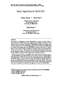
Algorithm VBP-D3(G = (V, E), S, Col) Input: An undirected multigraph G = (V, E) with maximum degree 3, whose vertices have been colored. Here n is the number of vertices in the input graph. Initially the algorithm is called with S ← ∅ and Col(v) = good for all vertices v ∈ G(V ). Output: A minimum odd cycle transversal of G. Step 1 Call P (G, S, Col). If P returns NO then return NO. Step 2 Apply the first step which is applicable: Step 2a Let n0 be the number of vertices in the current graph. If n0 ≤ 0.6n or if every path of length 2 has at least one bad vertex then try all possible solutions S ∪ T , where T is a some subset of the remaining good vertices, and return the one with minimum size. Step 2b Pick a path xyz in G where all of x, y, and z are good. Call the algorithm on the following instances and return the smaller solution. • S ← S ∪ {z} and call VBP-D3(G − {z}, S, Col). • Set Col(z) = bad and call VBP-D3(G, S, Col).
Fig. 1.
Algorithm VBP-D3()
B IPARTIZATION problems in maximum degree 4 graphs. Note that the F EEDBACK V ERTEX S ET problem is polynomial time solvable in maximum degree 3 graphs [14], but is NP-complete for maximum degree 4 graphs. The paper is organised as follows. In Section II, we present exact algorithms for the V ERTEX B IPARTIZATION problem in graphs with maximum degrees 3 and 4, and the F EEDBACK V ERTEX S ET problem in graphs with maximum degree 4. In Section III, we develop a general technique by which we can convert a parameterized algorithm of time complexity O∗ ((4 − �)k ), � > 0 to an exact algorithm of time complexity O ∗ ((2 − η)k ), η > 0. This technique is based on a careful use of the parameterized algorithm for certain values of the parameter and a brute-force algorithm for other values. In Section III-A, we give several applications of our results. In particular, we give the best known exact algorithms for the following problems: 1) V ERTEX B IPARTIZATION in general undirected graphs; 2) 4-H ITTING S ET; 3) F EEDBACK A RC S ET in tournaments. Apart from this, we also give simple efficient exact algorithms for the M AX C UT problem in graphs with average vertex degree 3 and 4 and for the 3-H ITTING S ET problem; these are not the best known exact algorithms for these problems but are stated in this paper to highlight the applicability of our results. Finally in Section IV, we conclude with some remarks and open problems. All graphs in this paper are undirected unless stated otherwise. II. Exact Algorithms for Vertex Bipartization and Feedback Vertex Set in Graphs with Maximum Degree 4 In this section, we give improved exact algorithms for the V ERTEX B IPARTIZATION problem in graphs of maximum degrees 3 and 4, and the F EEDBACK V ERTEX S ET problem in graphs of maximum degree 4. The main idea behind these algorithms is to use the techniques of preprocessing and branching. Typical branch-and-bound algorithms (for I NDEPENDENT S ET, V ERTEX C OVER) build a solution by either picking a vertex or excluding it from the solution. When they exclude a vertex from the solution they typically delete it and work on the resulting smaller graph. For the problems we work on, when we exclude a vertex from the solution we cannot delete it, because removing it may kill cycles passing through it. To overcome this, we resort to coloring the vertices. All vertices are colored good initially. When we branch on a good vertex, we either include it in our solution and delete it, or exclude it and color it bad. Coloring a vertex bad decreases the number of good vertices. As we always branch on good vertices we end up reducing the graph size in both cases. Just doing this gives us an O ∗ (2n ) algorithm. Our main contribution is in pushing this idea to get an O ∗ (cn ) algorithm where c < 2. In all the algorithms to follow Col is a function from the vertex set of the input graph to the set {good, bad} A. Vertex Bipartization in Graphs with Maximum Degree 3 The algorithm first preprocesses the graph using a preprocessing algorithm P (see Figure 2) and then either does a brute-force enumeration or finds a path xyz of length two consisting only of good vertices and branches on z. The algorithm is depicted in Figure 1.
3
Preprocessing Algorithm P (G, S, Col) Input: A multigraph G whose vertices have been colored good or bad along with a partially constructed solution S. Output: A (possibly smaller) colored multigraph along with a (possibly larger) solution or NO signifying that there does not exist a solution containing good vertices only. Let B be the set of bad vertices of G. Perform each of the following steps as long as possible. 1) If G has a vertex of degree ≤ 1, remove it along with the incident edge. 2) Check whether G[B] is bipartite. If not then return NO. 3) Check whether any connected component is a cycle. Remove all connected components that are even cycles; if a connected component C is an odd cycle, include a good vertex of C in S and remove this cycle. 4) If G has a vertex vi of degree 2 (which is not a self-loop) then it must be that vi is part of some path of the form uv1 . . . vi . . . vk w where each vj 1 ≤ j ≤ k is a degree 2 vertex and degree of u and w are ≥ 3. Here u and w could be the same vertex. a) Case 1: At least one of the vertices u and w are colored good. If the path length (k + 1 above) between u and w is odd then delete all the vertices v j and add the edge (u, w) (although u and w might already have an edge between them). If the path length between u and w is even then delete vertices v2 , v3 , . . . , vk and add an edge between v1 and w and color v1 bad. b) Case 2: Both u and v are colored bad. Suppose the path length (k + 1 above) is even and there is at least one vi colored good, then replace the path uv1 v2 . . . vk w by uvi w. If no vertex vi is colored good then replace the path uv1 v2 . . . vk w by uv1 w. Next suppose the path length is odd. If there is a good vertex v i then replace the path uv1 v2 . . . vk w by uvi vj w, where i 6= j and color vj bad if it is not already so. If there are no good vertices then replace the path uv1 v2 . . . vk w by the edge uw. (See Figure 3 for an explanation.) 5) Include all vertices with self loops in S and remove them from the graph. Also remove degree 2 vertices from all cycles of length 2. Find all triangles ∆uvw with Col(u) = good, Col(v) = bad, Col(w) = bad. Set S ← S ∪ {u} and remove u from the graph.
Fig. 2.
The preprocessing algorithm for the V ERTEX B IPARTIZATION problem
u
v1
vi
vk
w
u
w
u
v1
w
u
v1
vi
u
vi
w
Case 1: u is good and k + 1 is odd. u
v1
vi
vk
w
Case 2: u is good and k + 1 is even. u
v1
vi
vk
w
Case 3: vi is good and k + 1 is odd. u
v1
vi
vk
w
Case 4: vi is good and k + 1 is even.
Fig. 3.
Step 4 of the Preprocessing Algorithm P . The black vertices are bad and the shaded ones are good.
w
4
Correctness Step 2a of the algorithm VBP-D3 simply does a brute-force enumeration. In Step 2b, the algorithm branches on a good vertex z and constructs two solutions: one containing z and one not containing z and returns the one with minimum size. Both these steps do not need any further justification. We only need to justify the steps of the preprocessing algorithm P. In Step 1 of the preprocessing algorithm, we recursively remove vertices of degree ≤ 1. Such vertices cannot be part of any minimum solution and can be safely removed. In Step 2, we check whether the subgraph G[B] induced by the bad vertices contains an odd cycle. If this is the case, then there cannot be a minimum solution containing good vertices only. Thus P returns NO. The correctness of Step 3 is obvious. We next consider Step 4 in detail. In this step, we look for a vertex v i of degree 2 which does not have a self-loop. Such a vertex must be part of some path uv1 . . . vi . . . vk w, where u and w are of degree 3 and are possibly identical. There are two broad cases to handle: Case 1: At least one of u or w is colored good. Without loss of generality assume that Col(u) = good. Every odd cycle that passes through vi also passes through u and w. Thus if there is a good vertex vj that is part of some minimum solution S, then (S \ {vj }) ∪ {u} is also a minimum solution. Therefore we can label all the vertices v j bad, (1 ≤ j ≤ k). We would also like to maintain the parity of all cycles passing through u (and w). Thus if the path length is even we retain only one of the vertices vj and add the edges (u, vj ) and (vj , w); if the path length is odd we delete all the vertices v and add an edge between u and w. Case 2: Both u and w are colored bad. If the path P1k = v1 . . . vk does not have any good vertex then we only need to worry about maintaining the parity of the cycles passing through it and hence this case is similar to Case 1. But if P 1k has a good vertex, say vi , then not only do we need to maintain parity of the cycles passing through it but we also need to retain at least one good vertex from this path. This is because the good vertices on P 1k could be the only good ones on the odd cycles passing through it. We retain exactly one good vertex since any optimal solution contains at most one good vertex from this path. Hence if P1k is an odd length path then we retain vi and another vertex vj and add the edges (u, vi ), (vi , vj ), and (vj , w), and we color vj bad. Else, we retain only vi and add the edges (u, vi ), (vi , w). In Step 5, we add vertices having self-loops in our solution. This is because vertices with self-loops represent an odd cycle in the original graph and therefore must be included in any minimum solution. A similar argument holds for triangles containing only one good vertex. A degree 2 vertex which is part of a length 2 cycle can be safely removed from the graph since such a vertex cannot be part of the solution as it is not part of any odd cycle in the current graph. Time Complexity Let G = (V, E) be the input graph of maximum degree 3 with n vertices and m edges. Since the graph is of maximum degree 3, m ≤ 3n 2 . First we will show that if we reach Step 2a of the algorithm the number of good vertices n 0 in the current graph is at most 0.6n. To do this we partition the set of good vertices into following three types. Type 1:Degree 2 good vertices. Type 2:Degree 3 good vertices with one good neighbour. Type 3:Degree 3 good vertices with all bad neighbours. Step 4 of the preprocessing routine ensures that any degree 2 good vertex u has both its neighbours bad. Also observe that a good vertex of degree 3 can have at most one good neighbour; for if not then there exists a path of length 2 containing only good vertices. Thus any good vertex will be of one of the three types mentioned above. Let n 1 , n2 , and n3 be the number of vertices of Type 1, Type 2, and Type 3 respectively. We obtain an upper bound on the number of good vertices by counting the number of edges between good and bad vertices. Define ng = n1 + n2 + n3 . Define a good-bad edge to be one with one end point labelled good and the other labelled bad. Similarly define a good-good edge. The number of good-bad edges in the current graph is 2n1 + 2n2 + 3n3 and the number of good-good edges is n2 /2. Moreover the graph has maximum degree 3. We therefore have the following inequalities. 3(n − n1 ) + 2n1 n2 − 2 2 3n 2.5(n1 + n2 + n3 ) ≤ ⇒ ng ≤ 0.6n. 2 In Step 2b, we find a path xyz of length 2 consisting of good vertices only. Here we have two situations to deal with. If we include the vertex z in the solution, we remove it from the graph which results in at least one good vertex y with degree at most 2 having a good neighbour x. But the preprocessing algorithm will either delete y or label it bad. In either case, the number of good vertices reduces by at least 2. If we don’t pick z in our solution, then we label it bad, and this reduces the number of good vertices by 1. Thus the time complexity of the algorithm is bounded by the recurrence below: 2n1 + 2n2 + 3n3
≤
T (ng ) ≤ T (ng − 1) + T (ng − 2) T (0.6ng ) = 20.6ng . Here T (ng ) is bounded by (1.62)0.4ng ·20.6ng which is O∗ (1.8384ng ). Moreover on any path in the recursion tree, the algorithm takes polynomial space. Initially ng = n and therefore we have the following.
5
Preprocessing Algorithm P 1(G, S, Col) Input: A multigraph G whose vertices have been colored good or bad along with a partially constructed solution S. Output: A (possibly smaller) colored multigraph along with a (possibly larger) solution or NO signifying that there does not exist a solution containing good vertices only. Let B be the set of bad vertices of G. Perform each of the following steps as long as possible. 1) If G has a vertex of degree ≤ 1, remove it along with the incident edge. 2) Check whether G[B] is acyclic. If not then return NO. 3) Check whether any connected component is a cycle. If a connected component C is a cycle, include a good vertex of C in S and remove this cycle. 4) If G has a vertex vi of degree 2 (which is not a self-loop) then it must be that vi is part of some path of the form uv1 . . . vi . . . vk w where each vj 1 ≤ j ≤ k is a degree 2 vertex and u and w are vertices of degree ≥ 3. Here u and w could be the same vertex. a) Case 1: At least one of the vertices u and w is colored good. Then delete all the vertices vj and add the edge (u, w) (although u and w might already have an edge between them). b) Case 2: Both u and v are colored bad. Suppose there is at least one v i colored good, then replace the path uv1 v2 . . . vk w by uvi w. If no vertex vi is colored good then replace the path uv1 v2 . . . vk w by the edge uw. 5) Include all vertices with self loops in S and remove them from the graph. Find all cycles of length 2 with a good vertex and include it in S and remove it from the graph. Find all triangles ∆uvw with Col(u) = good, Col(v) = bad, Col(w) = bad. Set S ← S ∪ {u} and remove u from the graph.
Fig. 4.
The preprocessing algorithm for the F EEDBACK V ERTEX S ET problem
Theorem 1: Let G = (V, E) be an undirected graph with maximum degree 3 with n vertices and m edges. Then V ERTEX B IPARTIZATION problem on G can be solved exactly using polynomial space and in time O ∗ (1.8384n). B. The FVS and VBP problems in graphs with maximum degree 4 In this subsection, we extend the ideas described previously for the V ERTEX B IPARTIZATION problem to graphs with maximum degree 4. We also give an exact algorithm for F EEDBACK V ERTEX S ET problem on graphs with maximum degree 4. Again both algorithms in this subsection rely on preprocessing and branching. We will use the same preprocessing algorithm for the V ERTEX B IPARTIZATION problem. The preprocessing algorithm for F EEDBACK V ERTEX S ET is almost the same and is described in Figure 4. We first describe the algorithm for the F EEDBACK V ERTEX S ET problem. The main strategy of the algorithm is to find a good vertex with a sufficient number of good neighbours so that on the branch where we include a good vertex v in the solution, we can either delete at least one good neighbour of v or color the neighbour bad without making any further branches. The detailed algorithm is described in Figure 5. Correctness The argument for correctness closely follows the one given for the V ERTEX B IPARTIZATION problem in the previous section and is omitted. Time Complexity We will now analyze all cases handled by the algorithm carefully and bound the overall time taken by it. We claim that in Step 2a, the number of good vertices is bounded by 2n/3. If we reach Step 2a then either n 0 ≤ 2n/3 or every good vertex of degree three has at most one good neighbor and every good vertex of degree four has at most two good neighbours. In the case when n0 ≤ 2n/3, our claim follows trivially since the number of good vertices is ≤ n 0 . As for the second case, we can bound the number of good vertices by counting the number of edges between good and bad vertices. We can have following types of good vertices: Type 1Degree 2 good vertex (with both its neighbours bad). Type 2Degree 3 good vertex with one good neighbour. Type 3Degree 3 good vertex with all its neighbours bad. Type 4Degree 4 good vertex with two good neighbours. Type 5Degree 4 good vertex with one good neighbour. Type 6Degree 4 good vertex with all its neighbours bad. It should be clear that any good vertex at this stage falls in one of the types mentioned Let n i represent the number of Pabove. 6 good vertices of Type i and let ng be the total number of good vertices. Then ng = i=1 ni .
6
Algorithm FVS-D4(G = (V, E), S, Col) Input: A multigraph G = (V, E) with maximum degree 4, whose vertices have been colored. Here n is the number of vertices in the input graph. Initially the algorithm is called with S ← ∅ and Col(v) = good for all vertices v ∈ G(V ). Output: A minimum feedback vertex set of G. Step 1 Call P 1(G, S, Col). If P 1 returns NO then return NO. Step 2 Apply the first step which is applicable: Step 2a Let n0 be the size of the current graph. If n0 ≤ 2n/3 or if every good vertex v of degree 3 has at most one good neighbor and if every good vertex v of degree 4 has at most two good neighbours, then use brute-force and try all possible solutions S ∪ T , where T is some subset of the good vertices of the current graph, and return the one with minimum size. Step 2b Find a vertex u of degree 3 with at least two good neighbours, say v and w. Call the algorithm on following instances and return the smaller solution. • Set S ← S ∪ {v} and call FVS-D4(G − {v}, S, Col). • Set Col(v) = bad and call FVS-D4(G, S, Col). Step 2c Find a vertex u of degree 4 with at least 3 good neighbours, say v, w and z. Here we consider three cases and branch accordingly: 1. v is not part of the solution, 2. both v and w are part of the solution, and 3. v is part of the solution but w isn’t and return the smallest solution. • Set Col(v) = bad and call FVS-D4(G, S, Col). • Set S ← S ∪ {v, w} and call FVS-D4(G − {v, w}, S, Col). • Set S ← S ∪ {v} and Col(w) = bad and call FVS-D4(G − {v}, S, Col).
Fig. 5.
Algorithm FVS-D4()
We will now count the number of good-bad edges in the graph. The total number of good-bad edges is 2n 1 + 2n2 + 3n3 + 2n4 + 3n5 + 4n6 . It is easy to see that the quantity n2 + 2n4 + n5 counts every good-good edge twice. Thus number of good-good edges is (n2 + 2n4 + n5 )/2. Hence, 2n1 + 2n2 + 3n3 + 2n4 + 3n5 + 4n6
≤
4(n − n1 − n2 − n3 ) + 3(n2 + n3 ) + 2n1 2 n2 2n4 n5 − − − 2 2 2
A simple calculation shows that 3ng ≤ 2n from which it follows that ng ≤ 2n 3 This shows that number of good vertices in Step 2a is bounded by 2n/3. In Step 2b, we have a good vertex u of degree 3 that has at least two good neighbors v and w. When we include v in the solution, the degree of u becomes 2 and since it has a good neighbour w it is either removed or labelled bad by the preprocessing step. Thus we end up eliminating at least two good vertices from the graph. If we do not include v in the solution, we label it bad and end up decreasing the number of good vertices by one. Then we have T (ng ) ≤ T (ng − 1) + T (ng − 2). In Step 2c, we have a vertex u of degree 4 with at least three good neighbours v, w and z. We branch on three cases: 1) v is not in the solution, 2) v and w are in the solution, and 3) v is in the solution but w isn’t. In the first case, v is labelled bad and the number of good vertices reduces by at least 1. When both v, w are part of the solution then, on removing them, u has degree 2 and since it has a good neighbour z it is either removed or labelled bad by the preprocessing step. Thus we eliminate at least 3 good vertices in this case. In the last case, v is removed from the graph and w is labelled bad, which reduces the number of good vertices by at least 2. Thus we have the following recurrence on the number of good vertices. T (ng ) ≤ T (ng − 1) + T (ng − 2) + T (ng − 3). Combining the above, we get the following recurrence for the problem in the worst case, modulo the polynomial time used at
7
Algorithm Exact(Q,A ,c) (Q is a minimization problem and A is the FPT algorithm that solves its parameterized version in time O ∗ (ck ), where c is a constant and k is a parameter. Here n is the input size.) � n Compute λ from the equation cnλ = n−λn . for i = 1 to λn use the FPT algorithm A for Q to check whether there is solution of size i; if yes output i and halt. for i > λn use brute-force to check whether there exists a solution of size i; if yes, then output i and halt.
Fig. 6.
Algorithm Exact()
every node to find the vertex of required type. T (ng ) ≤ T (ng − 1) + T (ng − 2) + T (ng − 3) T (2ng /3) = 22ng /3 T (ng ) is bounded by (1.8393)ng /3 · 22ng /3 which is O∗ (1.945ng ). Setting the initial value of ng as n we get the following theorem. Theorem 2: Let G = (V, E) be an undirected graph with maximum degree 4 with n vertices and m edges. Then the F EEDBACK V ERTEX S ET problem on G can be solved exactly using polynomial space and in time O ∗ (1.945n ). We can modify our algorithm for the F EEDBACK V ERTEX S ET presented above for the V ERTEX B IPARTIZATION problem in graphs of maximum degree 4. The only modification we need to do is to call the preprocessing algorithm for V ERTEX B IPARTIZATION problem in Step 1. This gives us following theorem. Theorem 3: Let G = (V, E) be an undirected graph with maximum degree 4 with n vertices and m edges. Then the V ERTEX B IPARTIZATION problem on G can be solved exactly using polynomial space and in time O ∗ (1.945n ). III. Using FPT algorithms to design exact algorithms In the last section, we gave efficient algorithms for V ERTEX B IPARTIZATION and F EEDBACK V ERTEX S ET, but they critically used the fact that the maximum degree of the graphs is 3 or 4. Here we give a general technique of designing exact algorithms using parameterized algorithms as a subroutine and apply it to several problems. Let Q be an NP-optimization problem and suppose that it’s parameterized version3 (Q, k) is fixed parameter tractable. Let us also suppose that the FPT algorithm A for (Q, k) has a time complexity of the form O ∗ (ck , where k is the parameter, and c is a constant. This algorithm A immediately gives us an exact algorithm for Q with time complexity O ∗ (cn ), where n is an upper bound on the optimum solution size. What is interesting is that the FPT algorithm can actually give us an exact algorithm for Q with time complexity O ∗ (dn ), where d < c. Moreover, if c < 4 then we will show that d < 2. This fact has an interesting consequence. There are many optimization problems such as M AX I NDEPENDENT S ET, M IN V ERTEX C OVER, M IN F EEDBACK V ERTEX S ET which have trivial brute-force enumeration algorithms of time complexity 2 n . If the parameterized versions of any of these problems is solvable in time O ∗ (ck ), where c < 4 then we immediately obtain exact algorithms for these problems which are better than the trivial brute-force algorithms. We will show that this technique simplifies exact algorithms for many optimization problems and for some (e.g. V ERTEX B IPARTIZATION) gives the best known exact algorithm. Our algorithm makes clever use of the FPT algorithm A and brute-force enumeration. Consider a problem such as � Pi=n n ∗ V ERTEX B IPARTIZATION. Had we used brute-force throughout, then the time complexity would have been O ( i=0 i ) � n = O∗ (2n ). It is well known that the function i � increases with increasing i, attains a maximum at i = n/2, and then � n n decreases. Also, it is symmetric in that i = n−i . �Brute-force pushes the time complexity to O ∗ (2n ) because it is costlier n to search exhaustively when i is near n/2, since n/2 ≈ 2n . Therefore, if we adopt the strategy of using brute-force only for those values of i which are far removed from n/2 and using the FPT algorithm A for the remaining i values (that is, those near n/2), then we might end up with an exponential time complexity better than that of A . And indeed we do. Our algorithm is given in Figure 6. For simplicity the algorithm considers minimization problems only. For maximization problems we can modify the algorithm to output the largest i for which there exists a solution. 3 The parameterized version of an NP-optimization problem Q is defined as the language Q par which consists of pairs of the form hx, ki, where x is an instance of Q and k = opt(x).
8
Suppose the FPT algorithm A for Q takes O ∗ (ck ) time, where c is some constant. Then from the description of Algorithm Exact, it is easy to observe that its time complexity is upper bounded by following: � � � ��� n (1) O∗ max cλn , n − λn
Now suppose that the trivial brute-force algorithm for Q has time complexity O ∗ (2n ). We show that if we want Algorithm Exact to beat this trivial time bound then �we must have c < 4. We need a lemma. n is bounded by dn , where d is some constant < 2. Lemma 1: Let 12 < λ < 1. Then n−λn Proof: We know that � � � � � �λ � �1−λ !n n nn n 1 1 = ≤ = n − λn λn λ 1−λ (λn)λn ((1 − λ)n)(1−λ)n One can easily verify using calculus that the function �1−λ � �λ � 1 1 (0 < λ < 1) h(λ) = λ 1−λ attains a maximum of 2 at λ = 1/2. At other points in the interval ( 12 , 1) it has a value less than 2. This proves the claim. Equating cλ and h(λ) = d we get c = {h(λ)}1/λ < 21/λ . Since 1/2 < λ < 1 we see that c < 4. Also note that d = cλ < c. We thus have the following theorem. Theorem 4: Let Q be an NP-optimization problem and let n be an upper bound on the optimum solution size of Q such that a trivial brute force algorithm for Q takes time O ∗ (2n ). Suppose also that the parameterized version of Q is FPT with time complexity O ∗ (c k ) for some c < 4. Then there is an exact algorithm for Q with time complexity O ∗ (d n ) for some d < c and d < 2. A. Applications
In this section, we apply the algorithm developed in Section III to various problems and obtain exact algorithms with nontrivial worst-case time bounds. The problems for which we give efficient exact algorithms include the V ERTEX B IPARTIZATION problem in general undirected graphs, the 3 AND 4-H ITTING S ET problems, the F EEDBACK S ET problem in tournaments and the M AX C UT problem in graphs with average degree 3 and 4. Some of these results are new and some of them are given here to show the applicability of Theorem 4 and Algorithm Exact(). 1) Vertex Bipartization Problem.: We apply the algorithm developed in Section III to the V ERTEX B IPARTIZATION problem in general undirected graphs. This problem can be solved exactly in O ∗ (2|V | ) time. Reed, Kaleigh, and Vetta [12] have recently given an FPT algorithm for the parameterized version of this problem with running time O(3 k kmn). If we use their FPT algorithm directly to solve the optimum version of the problem we will take time O ∗ (3n ) which is worse than that taken by the trivial exponential time algorithm. However, if we use the algorithm in Figure 6 then with c = 3, we obtain λ = 0.6091 and get a running time of O ∗ (1.9526n). We therefore have the following theorem. Theorem 5: Let G = (V, E) be an undirected graph with n vertices then V ERTEX B IPARTIZATION problem can be solved in time O∗ (1.9526n). 2) 3- and 4-Hitting Set Problems.: The H ITTING S ET (HS) problem is defined as follows: Instance Goal
A finite family of sets S1 , S2 , . . . , Sm comprised of elements from a universal set U . Find a minimum sized subset T ⊆ U such that Si ∩ T 6= ∅ for all i.
The 3- and 4-HS problems are special cases of the H ITTING S ET problem. In the 3-HS problem |S i | (1 ≤ i ≤ m) is bounded by 3 and in the 4-HS problem by 4. The parameterized versions of these problems have been shown to be fixed parameter tractable by Neidermeier et al [8]. The main results in [8] can be summarized in the following theorem. Theorem 6: [8] The parameterized version of the 3-HS and the 4-HS problem can be solved in time O ∗ (2.27k ) and O∗ (3.3k ) respectively. We apply Algorithm Exact() to solve the 3- and 4-HS problems; the parameterized algorithm we use is the one by Neidermeier et al [8]. We get λ = 0.72 with c = 2.27 for the 3-HS problem and λ = 0.5721 with c = 3.3 for the 4-HS problem. This gives us the following theorem. Theorem 7: The 3- and 4-H ITTING S ET problems can be solved exactly in time O ∗ (1.80933)n and O∗ (1.9799n), where n = |U |. Recently Wahlstr¨om [15] proposed an exact algorithm for the 3-HS problem with time complexity O ∗ (1.6316n). The algorithm for the 3-HS problem in [15] does not directly generalize to the 4-HS problem. To the best of our knowledge our algorithm is the first exact algorithm for the 4-HS problem with the base of the exponent less than 2.
9
3) Feedback Set Problems in Tournaments.: The F EEDBACK A RC (V ERTEX ) S ET problem in directed graphs is defined as follows: Instance Goal
A directed graph G = (V, E). Find a minimum sized subset F ⊆ E (F ⊆ V ) such that G0 = (V, E − F ) (G0 = (V − F, E 0 )) is acyclic.
We will use the parameterized algorithms developed by Raman and Saurabh [10] for feedback set problems in tournaments. They give an O ∗ (2.415k ) and O∗ (2.27k ) algorithm for the F EEDBACK A RC S ET and the F EEDBACK V ERTEX S ET problem respectively. For the F EEDBACK A RC S ET problem in tournaments we get λ = 0.696 with c = 2.415; for the F EEDBACK V ERTEX S ET we get λ = 0.72 with c = 2.27. Then using Algorithm Exact() we obtain the following theorem. Theorem 8: Let G = (V, E) be a tournament with n vertices and m arcs. Then the minimum feedback arc set and feedback vertex set can be found in time O ∗ (1.84821m) and O∗ (1.80933n) respectively. Observe that in any directed graph, the size of the minimum feedback arc set is at most m/2. This fact ensures that Algorithm ∗ m/2 Exact() will never use brute-force as m ) 2 ≤ 0.696m. Hence the time complexity of the algorithm is bounded by O ((2.415) and therefore we get the following theorem. Theorem 9: Let G = (V, E) be a tournament with n vertices and m arcs. Then the minimum feedback arc set can be found in time O∗ (1.5541m). 4) Max Cut in graphs of average degree 3 or 4.: We will solve the M AX C UT problem using the parameterized algorithm for E DGE B IPARTIZATION developed by Niedermeier et al [7] and a lower bound on the size of the maximum cut. The parameterized algorithm for E DGE B IPARTIZATION presented in [7] has time complexity O(2 k · nO(1) ). Recall that an instance of the E DGE B IPARTIZATION problem is an undirected graph G = (V, E) and the question is to find a minimum set of edges that needs to be deleted from G to make it bipartite. The relationship between this problem and the M AX C UT problem is straightforward: the maximum cut in a graph is E − the minimum set of edges to make the graph bipartite. Thus solving the E DGE B IPARTIZATION problem is equivalent to solving � �the M AX C UT problem. 1 n−c + for maximum cut, where c is number of connected components and Poljak et al in [9] give a lower bound of m 2 2 2 m and n are, respectively, the number of edges and vertices in the graph. If G is a connected graph on n vertices and m edges with average degree 3, then m = 1.5n. The minimum number of edges to be removed from G to make it bipartite is then � � � � 3n n 1 m n−1 3n n − 1 m − |max cut| ≤ m − = = + . + − + 2 4 2 4 4 2 4 We use the parameterized algorithm in [7] to solve the E DGE B IPARTIZATION problem. Since λ = 0.773 for c = 2, Exact() will never use brute-force when the input graph has average degree 3, since in this case the solution size is bounded by n/2 as shown above. Because of the upper bound on the number of edges needed to be removed, we achieve a time complexity of O∗ (2n/2 ) = O∗ (1.414n). Had G been of average degree 4, then the upper bound on the number of edges to be deleted would be 3n/4 + 1/4. This upper bound is also less than 0.771m and hence Exact() will never use brute-force. So the time complexity of solving the E DGE B IPARTIZATION problem would be O ∗ (23n/4 ) = O∗ (1.6818n). We thus have the following theorem. Theorem 10: The Max Cut problem can be solved exactly in time O ∗ (1.4141n) in graphs with average degree 3 and in time O∗ (1.6818n ) in graphs with average degree 4. Both of these algorithms take polynomial space. Neidermeir et al [6] achieve the same time bound for graphs with maximum degree 3 and a better time bound of O ∗ (1.5871n) for graphs with maximum degree 4. IV. Conclusion In this paper, we have obtained improved exact algorithms for several problems including V ERTEX B IPARTIZATION in general undirected graphs, 4-H ITTING S ET, F EEDBACK V ERTEX S ET in graphs with maximum degree at most 4, and F EEDBACK A RC S ET in tournaments. We introduced two general techniques to obtain efficient exact algorithms. One of these is a modified version of the general branch-and-bound technique and the other one is based on parameterized complexity algorithms. Further reduction in the base of the exponent of all these algorithms remains open. It would be interesting to investigate the practical performance of these algorithms. Another major open problem is to devise an exact algorithm with time complexity less than O ∗ (cn ), c < 2 for the F EEDBACK V ERTEX S ET problem in general undirected graphs. Remark. After submitting this paper, we discovered an exact algorithm for V ERTEX B IPARTIZATION by Byskov [1], with time complexity O ∗ (1.8631n). However, we have improved this result substantially in [11]. R EFERENCES [1] J. M. B YSKOV. On the Number of Maximal Bipartite Subgraphs of a Graph. Journal of Graph Theory 48 (2): 127-135, (2005). [2] H. C HOI , K. N AKAJIMA AND C. S. R IM . Graph Bipartization and Via Minimization. SIAM Journal of Discrete Mathematics 2 (1): 38-47, 1989. [3] R. D OWNEY AND M. F ELLOWS . Parameterized Complexity. Springer-Verlag (1998).
10
[4] R. D OWNEY AND M. F ELLOWS . Parameterized Complexity for the Skeptic. In Proc. of 18th CCC : 147-169, 2003. [5] N. G ARG , V. VAZIRANI AND M. YANNAKAKIS . Approximate Max-Flow Min-(Multi) Cut Theorems and Their Applications. SIAM Journal on Computing 25 (2): 235-251, 1996. [6] J. G RAMM , E. A. H IRSCH , R. N IEDERMEIER AND P. R OSSMANITH Worst-case upper bounds for MAX-2-SAT with an application to MAX-CUT. Discrete Applied Mathematics 130 (2): 139-155, 2003. ¨ [7] J. G UO , J. G RAMM , F. H UFFNER , R. N EIDERMEIER AND S. W ERNICKE . Improved Fixed-Parameter Algorithms for Two Feedback Set Problems. To appear in the proceedings of 9th Workshop on Algorithms and Data Structures (WADS). Springer Verlag, Lecture Notes in Computer Science (2005). [8] R. N IEDERMEIER AND P. R OSSMANITH . An effiecient fixed parameter algorithm for 3-Hitting Set. Journal of Discrete Algorithms 1 (1): 89-102, 2003. [9] S. P OLJAK AND D. T URZIK . A Polynomial Algorithm for Constructing a Large Bipartite Subgraph, with an Application to a Satisfiability Problem. Canad. J. Math 34 (3): 519-524, 1982. [10] V. R AMAN AND S. S AURABH . Improved Parameterized Algorithms for Feedback Set Problems in Weighted Tournaments. In Proc. of the 1st International Workshop on Exact and Parameterized Algorithms (IWPEC):260-270, 2004. To appear in TCS. [11] V. R AMAN , S. S AURABH AND S. S IKDAR . Exact Algorithms for Odd Cycle Transversal and Other Problems. Technical Report, IMSC-2005-06-16, The Institute of Mathematical Sciences, (2005). [12] B. R EED , K. S MITH AND A. V ETTA . Finding Odd Cycle Transversals, Operations Research Letters 32 (2004) 299-301. [13] R. R IZZI , V. B AFNA , S. I STRAIL AND G. L ANCIA . Practical Algorithms and Fixed-Parameter Tractability for the Single Individual SNP Haplotyping Problem. WABI: 29-43, 2002. [14] S. U ENO , Y. K AJITANI AND S. G OTOH . On the Nonseparating Indepedent Set Problem and Feedback Set Problem for Graphs with no Vertex Degree Exceeding Three. Discrete Mathematics 72 (1988) 355-360. ¨ . Exact algorithms for finding minimum transversals in rank-3 hypergraphs. Journal of Algorithms 51(2): 107 - 121, 2004. [15] M. WAHLSTR OM [16] G. W OEGINGER . Exact algorithms for NP-hard problems: A survey. In Combinatorial Optimization—Eureka! You shrink! Springer LNCS 2570: 185-207, 2003. [17] X. Z HUNAG AND S. PANDE . Resolving Register Bank Conflicts for a Network Processor. In Proc. of 12th PACT: 260-278, 2003.