Bidirectional Best Hit r-Window Gene Clusters. Trong Dao Le, Melvin Zhang, and Hon Wai Leong. Department of Computer Science, National University of ...
Algorithms for Computing Bidirectional Best Hit r-Window Gene Clusters Trong Dao Le, Melvin Zhang, and Hon Wai Leong Department of Computer Science, National University of Singapore Computing 1, 13 Computing Drive, Singapore 117417, Republic of Singapore {daole,melvin,leonghw}@comp.nus.edu.sg
Abstract. Genome rearrangements are large-scale mutations that result in a shuffling of the genes on a genome. Despite these rearrangements, whole genome analysis of modern species has revealed sets of genes that are found close to one another in multiple species. These conserved gene clusters provide useful information on gene function and genome evolution. In this paper, we consider a novel gene cluster model called bidirectional best hit r-window (BBHRW) in which the idea is to (a) capture the “frequency of common genes” in an r-window (interval of at most r consecutive genes) of each genome and (b) to further strengthen it by the bidirectional best hit criteria. We define two variants of BBHRW using two different similarity measures to define the “frequency of common genes” in two r-windows. Then the algorithmic problem is as follows: Give two genomes of length n and m, and an integer r, compute all the BBHRW clusters. A straight-forward algorithm for solving this problem is an O(nm) algorithm that compares all pairs of r-windows. In this paper, we present faster algorithms (SWBST and SWOT) for solving these two BBHRW variants. Algorithm SWBST is a simpler algorithm that solves the first variant of the BBHRW, while algorithm SWOT solves both variants of the BBHRW. Both algorithms have running time O((n+m)r lg r). The algorithmic speed-up is achieved via a sliding window approach and with the use of efficient data structures. We implemented the algorithms and compare their running times for finding BBHRW clusters conserved in E. coli K-12 (2339 genes) and B. subtilis (2332 genes) with r from 1 to 30 to illustrate the speed-up achieved. We also compare the two similarity measures for these genomes to show that the choice of similarity measure is an important factor for this cluster model.
1
Introduction
In the course of evolution, the genome of a species undergoes large-scale, rare mutation events known as rearrangements [7]. Despite the shuffling of genes due to rearrangements, comparison of modern species reveals that certain sets of genes always occur near one another in several genomes. These gene sets are commonly known as conserved gene clusters. We model a chromosome as a string where each character represents a gene family. Genomes with multiple chromosomes are handled by concatenating the M. Atallah, X.-Y. Li, and B. Zhu (Eds.): FAW-AAIM 2011, LNCS 6681, pp. 275–286, 2011. c Springer-Verlag Berlin Heidelberg 2011 �
276
T.D. Le, M. Zhang, and H.W. Leong
different chromosomes together in an arbitrary order. An important feature of many gene cluster models is that the order of occurrence of the elements in a cluster does not matter. Hence, when looking for instances of a given cluster in a string, we are only interested in the set of characters. This is known as the character set of a string [3]. One of the simplest gene cluster model is the common interval model [9]. A common interval is a set of characters and it occurs in a string S if it is the character set of some substring of S. The common interval model only considers character sets of substrings. Thus it assumes that a elements of a cluster are contiguous. When the strings are permutations of n characters, there is an O(kn + C) time algorithm [9,5] for finding all C common intervals that occur in k strings. The best known algorithm for finding common intervals in general strings is an O(N 2 ) time algorithm [3], where N is the total length of all the strings. The common interval model assumes that a gene cluster is contiguous. However, gene clusters evolve over time and may gain/loss elements in different genomes. Therefore, one possible generalization is to allow clusters to form subsequences instead of substrings. Since clusters are relatively compact structures, the gene team model considers character sets of gapped subsequences with gaps of at most δ characters. There is an O(kn lg n) time algorithm of the case of k permutations [1] and an O(nk ) time algorithm for k sequences [4]. The preceding models (common intervals and gene teams) look for character sets that occur in a set of strings. An alternative solution to define clusters that are not contiguous is to look for substrings with similar characters sets. Motivated by the popular bidirectional best hit criteria [6] for finding corresponding genes in several species, we propose a novel gene cluster model based on finding bidirectional best hit substrings of at most r characters. The underlying assumption is that substrings in two different strings are instances of the same cluster if their character sets are bidirectional best hits. We consider two variants of this model, based on two similarity measures for strings: count(wG , wH ) is the number of characters in wG that occur in wH , and msint(wG , wH ) is the size of the multiset intersection of wG and wH . A na¨ıve algorithm that computes all clusters by comparing all pairs of substrings requires at least quadratic time. Exploiting the structure of the similarity measures, we designed two O((n + m)r lg r) time algorithms, where n and m are the lengths of the two input strings.
2
Problem Formulation
We model the sequence of genes on a genome as a string over the alphabet Σ of gene families. Given a string S, S[i, j] denotes a substring of S that starts at position i, ends at position j, and includes both S[i] and S[j]. Gene clusters are compact structures, hence we only consider substrings of length at most r, where r is a user defined parameter. Definition 1 (r-window). An r-window of a string G is a substring of G with at most r characters.
Computing Bidirectional Best Hit r-Window Gene Clusters
277
For a given r-window wG of a string G and a specific similarity measure, we want to find r-windows of another string H that is the most similar to wG . We call these the best hits of wG . Definition 2 (Best hits of a r-window). Given an r-window wG on a string G, a string H, and a similarity measure sim, the best hits of wG are the rwindows wH of H that satisfies � � sim(wG , wH ) > sim(wG , wH ) for all wH which does not contain wH
Depending on the definition of the similarity measure, it is possible for a given rwindow wG there are two or more r-windows of H that have the same similarity to wG . In the case where one of these r-window contains the other, we prefer � the minimal one. That is why in the above definition, we require that wH does not contain wH . Naturally, we want to find a pair of r-windows that are the unique best hit of each other. Hence, we define bidirectional best hits as follows: Definition 3 (BBH r-window cluster). Given two strings G and H, a window size r, and a similarity measure sim, a pair of r-windows (wG , wH ) is a bidirectional best hit r-window cluster if and only if wG is the only best hit of wH with respect to sim and wH is the only best hit of wG with respect to sim. The computational problem we are solving is to find all occurrences of BBH r-window cluster. Formally, given two strings, G and H, a similarity measure between a pair of windows, sim, and a maximum window length, r, we want to compute the set of all BBH r-window clusters. A na¨ıve algorithm for the above problem is compare all r-windows of string G against all r-windows of string H. This is a general algorithm since it does not depend on the form of the similarity measure, but it requires at least quadratic time. In the following, we consider two specific similarity measures and exploit the specific properties of the similarity measures to design more efficient algorithms for computing all BBHRW clusters.
3
BBHRW Using Similarity Measure count
3.1
Similarity Measure count
The first similarity measure we will consider is count1 . count(wG , wH ) is the number of characters in wH that are also in wG . Formally, count(wG , wH ) = |{p | wH [p] ∈ CS(wG )}| where CS(wG ) is the character set of wG . This is an asymmetric function since we consider all the characters in wH but treat characters in wG as a set. For example, count(abc, aab) is 3 due to one character a and one character b in aab. In contrast, count(aab, abc) is 2 since c is not in aab. 1
Applications and comparison of BBHRW (count) with the gene teams model was discussed in [10].
278
3.2
T.D. Le, M. Zhang, and H.W. Leong
Algorithm SWBST
Our algorithms for computing BBHRW clusters for two strings G and H consists of three main steps: 1. computing best hits of r-windows in G 2. computing best hits of r-windows in H 3. keeping only the bidirectional best hits The most time-consuming step is computing the best hits. We then store the best hit for H in a hash table and iterate over the best hits for G, keeping only the bidirectional best hits. In the following, we will focus on how we compute the best hits of r-windows in G. Key ideas. We observe that for a given r-window wG in G, most of the rwindows in H do not have any characters in common with wG since only some of the characters in H are also in wG . Our approach is to represent the characters in H that are also in wG in a data structure that allows us to query for the best hit efficiently. There are O(nr) r-windows in G so building this data structure for every r-window is time-consuming. The key is to enumerate the r-windows in G in a specific order. For every position in G, we consider the r-windows that starts at that position in increasing length. This is because the r-window of length l that starts at position i is just the r-window of length l − 1 starting at position i with an addition character. Suppose we have computed the data structure for the characters in H in the current r-window and found the best hit, the next r-window is the previous one with an additional character. This means that we can update our data structure by inserting the additional characters instead of computing it from scratch. Finding best hits. The specific data structure we are using is an augmented binary search tree which supports range query. Each node in the tree is a character in H that is also in the current r-window. We order the nodes according to their position in H. We augment each node u, with s = count(wG , H[p, p + r − 1]), where p is the position of u, and maxs , the maximum value of s in the subtree rooted at u. This gives us a simple algorithm to find the best hit by starting from the root and following the node with the largest maxs . If we find more than one node with the largest maxs than we can stop, since the best hit is not unique. Inserting additional characters. The main difficulty is in updating our binary search tree when we want to add an additional character. Since our data structure only considers characters in H that are also in wG , count(wG , H[p, p+ r − 1]) is also the number of nodes in the tree whose position is in [p, p + r − 1]]. In order to add a new node at position p, we first compute the value of s for the new node by counting the number of nodes in the tree whose position is in [p, p + r − 1]. Secondly, we increase the value of s by 1 for those nodes in the tree whose position is in [p − r + 1, p]. In both cases, we need to deal with
Computing Bidirectional Best Hit r-Window Gene Clusters
279
nodes in a certain range. Hence, we further augment each node with the range of positions of the characters in its subtree (minp and maxp ) and a value (Δ) that indicates the increase to the value of s in all nodes in this subtree. These allows us to execute range queries and updates efficiently. The details are given in the next section. In summary, the algorithm for insertion consist of the following three steps: 1. compute the similarity measure s of the new node using a range query to count the number of nodes in a given interval 2. update the nodes affected by the new node using a range update 3. insert the new node into the binary search tree Range query and update algorithm. An interval of a node u is the interval [minp , maxp ].
1 2 3 4 5 6 7 8 9 10 11 12 13 14 15
Data: a node u in the tree, an interval [s, e] to query/update Result: update the subtree rooted at u and return the answer to the query if the interval of u lies inside [s, e] then ProcessSubtree: Query/update the attributes in this node end else if the position of u is in [s, e] then ProcessNode: Query/update the attributes in this node end if the interval of the left child of u intersects with [s, e] then Recursive call to the left child end if the interval of the right child of u intersects with [s, e] then Recursive call to the right child end CombineSubtree: Combine the result of the recursive calls and/or update the node to maintain consistency end Algorithm 1. Algorithm to query/update nodes in a given interval
We make use of the range query algorithm (Algorithm 1) to compute the result of a query or to update the similarity measure in an interval. Figure 1 shows a possible tree and the nodes visited during a range query operation. Let ProcessSubtree be the procedure to query/update the subtree rooted at u in line 2, ProcessNode be the procedure to query/update the node u in line 6, and CombineSubtree be the procedure in line 14. We use this algorithm to compute the similarity measure s for the new node and to update the data structure.
280
T.D. Le, M. Zhang, and H.W. Leong
Fig. 1. The nodes with bold outline are visited by Algorithm 1 during a range query on the interval [1, 5]
Our structure is based on the interval decomposition idea [2], hence, the worst case time complexity of the range query/update is O(lg |T |) where |T | is the size of the tree. Compute the similarity measure of the new node. Computing the similarity measure of the new node makes use of Algorithm 1 and the corresponding procedures are as follows: ProcessSubtree: return the number of nodes in the subtree. ProcessNode: add 1 to the result for this node. CombineSubtree: return the result plus the sum of the recursive calls. Update the similarity measure of affected nodes. Insertion of the new node increased the similarity measure for nodes in the interval [p − r + 1, p] by 1, where p is the new node’s position. Updating the similarity measure for affected nodes requires a range update. ProcessSubtree: increase Δ by 1 to indicate that the value of s in the subtree has increased by 1 without actually changing s in each node. ProcessNode: increase s by 1. CombineSubtree: update the maxs according to the value of maxs and Δ in the left and right subtrees. Insert the new node into the tree. Insertion a node follows the same procedure as a standard binary search tree. In case where rotations might be needed to keep the tree balanced, the augmented attributes of a node are updated using the attributes of its subtrees. 3.3
Time Complexity Analysis of Algorithm SWBST
For simplicity, we assume that the number of occurrences of a character in a string is bounded by a constant. In the worst case, the size of our binary search tree is O(r). Hence, all operations on the tree have a worst case time complexity of O(lg r) where r is the maximum window length.
Computing Bidirectional Best Hit r-Window Gene Clusters
281
Using the above data structure, the worst case time complexity to compute best hits for all r-windows with the same starting position in G is O(r lg r). We have to compute best hits twice: once from G to H which takes O(nr lg r) time and once from H to G which takes O(mr lg r). Hence, the worst case time complexity of the entire algorithm is O((n + m)r lg r) where n and m are the length of G and H.
4
BBHRW Using Similarity Measure msint
4.1
Similarity Measure msint
The earlier similarity measure count is an asymmetric function. In this section, we consider a symmetric similarity measure that takes into account the multiplicity of the characters. We make use of the multiplicity by using the character multiset instead of character set and let the similarity measure be the size of the multiset intersection. Let CMS(S) denote the character multiset of the string S. Then, the similarity measure msint is as follows: msint(wG , wH ) = |CMS(wG ) ∩ CMS(wH )| The following illustrates the difference between count and msint – count(abacf, bfcba) = 5 and msint(abacf, bfcba) = 4 – count(abacf, fcbaa) = 5 and msint(abacf, fcbaa) = 5 Observe that for the same pair of strings, the value of count is at least as large as msint. In the above example, bfcba and fcbaa give the same value under count, and fcbaa has a higher value compared to bfcba under msint. Intuitively, fcbaa is a more similar to abacf as both of them have two copies of the character a, whereas bfcba has two copies of character b but only a single copy of character a. This illustrates that we can better distinguish between two strings when we make use of the multiplicity of the characters. 4.2
Algorithm SWOT
The general approach for this algorithm is the same as in algorithm SWBST. The difference is in how we compute best hits. The method for computing best hits used in algorithm SWBST cannot be extended for msint because the range query used for counting the number of characters in an substring of H does not take into account the multiplicity of the characters. Hence, we need a new approach to handle the similarity measure msint. The key insight is that instead of storing the similarity measure in the data structure, we store the intervals to be updated. These intervals depend on the order of insertion, so we have to insert characters from left to right. We call these intervals the update interval of a character. Definition 4. An update interval of a character g is the interval where the similarity measure of every substring starting in the interval is increased by the addition of g.
282
T.D. Le, M. Zhang, and H.W. Leong
The key is to recast the problem of finding best hits to the problem of finding the position where the most number of update intervals overlap. This position is the start of the best hit r-window. We keep track of the update intervals using the segment tree data structure. Similar to the algorithm SWBST, we build the data structure incrementally for different r-windows by inserting new update intervals as the current r-window is extended by an additional character. Adding a single character to the current r-window may require inserting several update intervals since there may be multiple occurrences of the character in the string H. The algorithm for inserting a new character and computing best hits consist of three steps: 1. computing the update interval of a new character 2. inserting the update interval and updating the segment tree 3. determining the best hit Computing the update interval of a new character. As discussed earlier, inserting a new character increases the similarity measure of the r-windows containing the character. In the case of msint, the similarity measure increases by 1. The following gives the formula to compute the update interval for similarity measure msint. Definition 5 (Update interval for similarity measure msint). Let Hc denote a list of occurrence of character c in H in increasing order. Consider a character c at position p which has index k in Hc , its update interval is [max(1, p − r + 1, p� + 1), p] where l is the number of character c in wG and H[p� ] = c has index k − l in Hc . If k − l is less than 1, let p� be 0. Observe that every r-window whose start position is the interval [max(1, p−r), p] is affected by H[p] except those r-windows that already have enough character c. Position p� is the last position that has as many occurrences of character c as r-window wG , therefore any position at or before p� is not affected by the insertion of a character at position p. Figure 2 illustrates the update intervals for each character of the string H for a given r-window wG . Note that this formulation of the problem is also able to handle similarity measure count presented earlier. In the case of count, the update interval for a new character at position p is simply [max(1, p − r + 1), p]. From the above definition, we can compute the update interval of a character in constant time. Inserting the update interval and updating the segment tree. Insertion of the update interval follows from standard segment tree insertion. In order to compute the best hit efficiently, we augment each node to keep track of the maximum number of overlapping intervals in its subtree. This augmented value is updated during insertion.
Computing Bidirectional Best Hit r-Window Gene Clusters
283
Fig. 2. The update intervals corresponding to each characters of H = ababbc with the red line representing maximum overlapped points with respect to wG = abb and r = 5. There is no update interval for character c since it does not occur in wG .
Determining the best hit. Computing the region covered by the most number of update intervals incrementally is the dynamic version of the standard stabbing query problem [2]. In our case, since we know the maximum number of overlapping interval in the subtree of each node, we can simply start from the root of the segment tree and follow the child that has the larger maximum number of overlapping interval. The leaf node that we reach at the end of this process is the interval with the most overlap and equivalently the highest similarity measure according to msint. 4.3
Time Complexity Analysis of Algorithm SWOT
For simplicity, we assume that the number of occurrences of a character in a string is bounded by a constant. Consider two strings of length n and m respectively, pre-computing the lists of occurrences of a character in H for all characters in H takes O(m) time. Computing the update interval for each character takes O(1). The worst case time complexity of updating the segment tree and traversing the tree to find the start position of the best hit r-window is O(lg r) [2] as there are at most O(r) intervals in the tree. Therefore, the worst case time complexity for computing best hits in H for every r-window of G is O(m+nr lg r), which is the same as the method for computing best hits used in algorithm SWBST. Hence, the worst case time complexity of the entire algorithm is O((n + m)r lg r) (same as algorithm SWBST).
5
Results and Discussion
In this section, we are interested in the improvement in the running time of our algorithms compared to the na¨ıve algorithm and the difference between the two similarity measures. We have previously shown that the BBHRW (count) clusters have a greater correspondence to known biological structures than gene teams [10].
284
T.D. Le, M. Zhang, and H.W. Leong
In practice, we want to include domain specific knowledge about the clusters we are modelling. In the case of gene clusters, where clusters represents descendants of a common ancestor, overlapping clusters are not meaningful. Therefore, we introduce a post processing step to merge clusters when both windows overlap. 5.1
Experimental Setup
Our dataset consist of two prokaryotic genomes, namely E. coli K-12 (GenBank accession number NC000913) and B. subtilis (NC000964) downloaded from the NCBI Microbial Genomes Resource. We convert each genome into a string by representing each gene by its COG [8] label. There are 4289 genes in E. coli K-12 and 4100 genes in B. subtilis. After removing the genes that are unique to each genome, we obtain two strings of 2339 characters (E. coli K-12) and 2332 characters (B. subtilis) from an alphabet of size 1137 (COG labels). We computed the BBHRW gene clusters between the two genomes using both similarity measures for r ranging from 1 to 30 (on an Intel Core 2 Duo T7300 2Ghz with 2GB of RAM running Ubuntu 10.10). 5.2
Comparison of the Running Time
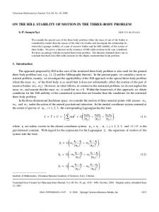
As shown in Figure 3, the running time of SWBST and SWOT are almost the same when we fix the two strings and increase r from 1 to 30. This is expected from their complexities. In contrast, running time of the na¨ıve algorithm is roughly quadratic with respect to r. From this result, we conclude that our algorithms are much more scalable than the na¨ıve algorithm. 5.3
Characteristics of BBHRW Clusters for count and msint
Figure 4 shows the number of clusters produced by our algorithm for the two similarity measures for r from 1 to 30. The two curves shows completely different Running time versus window size for similarity measure COUNT
Running time (seconds)
100
Running time versus window size for similarity measure MSINT 180
Naive algorithm SWBST SWOT
160 Running time (seconds)
120
80 60 40
Naive algorithm SWOT
140 120 100 80 60 40
20 20 0
0 5
10
15 20 Window size, r
25
30
5
10
15 20 Window size, r
25
30
Fig. 3. Comparison of the running time between the na¨ıve algorithm, algorithm SWBST and algorithm SWOT for the two similarity measures, count (left) and msint (right). Note that algorithm SWBST cannot be used for similarity measure msint.
Computing Bidirectional Best Hit r-Window Gene Clusters
285
Number of BBHRW clusters reported for each similarity measure 500
Number of BBHRW clusters
450
MSINT COUNT
400 350 300 250 200 150 100 5
10
15 20 Window size, r
25
30
Fig. 4. Number of reported BBHRW clusters for r varying from 1 to 30
trends. The number of results for similarity measure count peak at r equal to 13 and decreases slightly as r increases to 30. In contrast, for similarity measure msint the number of results increases with the parameter r. This phenomenon is due to the fact that msint is symmetric while count is not. When the similarity measure is symmetric, it is always possible to find a bidirectional best hit when starting from any pair of r-windows. Suppose (wG , wH ) is not a bidirectional best hit and without loss of generality assume that wG is not � which is the best hit the best hit of wH . Then, there exist another r-window wG � � of wH and msint(wG , wH ) is greater than msint(wG , wH ). If (wG , wH ) is not a bidirectional best hit, we simply repeat the previous argument. Each time we do this the similarity measure strictly increases. Since the similarity cannot increase indefinitely, we eventually reach a maxima and find a bidirectional best hit. The same argument cannot be applied to an asymmetric similarity measure because � � , wH ) is greater than count(wG , wH ), count(wH , wG ) may be while count(wG smaller then count(wG , wH ). Therefore, it is easier to find bidirectional best hits when the similarity measure is symmetric and this is reflected by the greater number of BBHRW clusters found using the similarity measure msint. In practice, we found that using r = 6 (for count) and r = 8 (for msint) results in the greatest number of BBHRW clusters that corresponds to known biological structures such as operons (data not shown).
6
Conclusion
We proposed the BBHRW gene cluster model and two variants based on different similarity measures. Similarity measure msint is symmetric and takes into consideration the number of copies of each gene, whereas count is asymmetric. We designed an efficient algorithm for each variant by making use of fast data structures that support incremental updates. In our experiments on real biological data, we discovered that using a symmetric similarity measure results in many more cluster being reported as compared to an asymmetric similarity
286
T.D. Le, M. Zhang, and H.W. Leong
measure. An interesting direction for future work is to investigate imposing other constraints or post-processing steps to filter or refine the clusters generated.
Acknowledgements We would like to thank the reviewers for their efforts in reviewing our paper and pointing out issues that need to be addressed. This work was supported in part by the National University of Singapore under Grant R252-000-361-112.
References 1. B´eal, M.P., Bergeron, A., Corteel, S., Raffinot, M.: An algorithmic view of gene teams. Theoretical Computer Science 320(2-3), 395–418 (2004) 2. Bentley, J.: Solutions to Klee’s rectangle problems. Unpublished manuscript, Dept. of Comp. Sci., Carnegie-Mellon University, Pittsburgh (1977) 3. Didier, G., Schmidt, T., Stoye, J., Tsur, D.: Character sets of strings. Journal of Discrete Algorithms 5(2), 330–340 (2007) 4. He, X., Goldwasser, M.H.: Identifying conserved gene clusters in the presence of homology families. Journal of Computational Biology 12(6), 638–656 (2005) 5. Heber, S., Stoye, J.: Finding all common intervals of k permutations. In: Amir, A., Landau, G.M. (eds.) CPM 2001. LNCS, vol. 2089, pp. 207–218. Springer, Heidelberg (2001) 6. Moreno-Hagelsieb, G., Latimer, K.: Choosing BLAST options for better detection of orthologs as reciprocal best hits. Bioinformatics 24(3), 319 (2008) 7. Sankoff, D.: Rearrangements and chromosomal evolution. Current Opinion in Genetics & Development 13(6), 583–587 (2003) 8. Tatusov, R.L., Natale, D.A., Garkavtsev, I.V., Tatusova, T.A., Shankavaram, U.T., Rao, B.S., Kiryutin, B., Galperin, M.Y., Fedorova, N.D., Koonin, E.V.: The COG database: new developments in phylogenetic classification of proteins from complete genomes. Nucleic Acids Research 29(1), 22–28 (2001) 9. Uno, T., Yagiura, M.: Fast algorithms to enumerate all common intervals of two permutations. Algorithmica 26(2), 290–309 (2000) 10. Zhang, M., Leong, H.W.: Bidirectional best hit r-window gene clusters. BMC Bioinformatics 11(suppl. 1), S63 (2010)