Hindawi Publishing Corporation Mathematical Problems in Engineering Volume 2013, Article ID 904768, 10 pages http://dx.doi.org/10.1155/2013/904768
Research Article New Algorithms for Bidirectional Singleton Arc Consistency Yonggang Zhang,1,2 Qian Yin,3 Xingjun Zhu,1,2 Zhanshan Li,1,2 Sibo Zhang,1,2 and Quan Liu2,4 1
College of Computer Science and Technology, Jilin University, Changchun 130012, China Key Laboratory of Symbol Computation and Knowledge Engineering of Ministry of Education, Jilin University, Changchun 130012, China 3 College of Computer Science and Information Technology, Northeast Normal University, Changchun 130117, China 4 School of Computer Science and Technology, Soochow University, Jiangsu 215006, China 2
Correspondence should be addressed to Yonggang Zhang;
[email protected] Received 23 June 2013; Accepted 4 September 2013 Academic Editor: William Guo Copyright © 2013 Yonggang Zhang et al. This is an open access article distributed under the Creative Commons Attribution License, which permits unrestricted use, distribution, and reproduction in any medium, provided the original work is properly cited. Bidirectional singleton arc consistency (BiSAC) which is an extended singleton arc consistency (SAC) has been proposed recently. The first contribution of this paper is to propose and prove two theorems of BiSAC theoretically (one is a property of BiSAC and the other is the property of allowing the deletion of some BiSAC-inconsistent values). Secondly, based on these properties we present two algorithms, denoted by BiSAC-DF and BiSAC-DP, to enforce BiSAC. Also, we prove their correctness and analyze the space and time complexity of them in detail. Besides, for special circumstances, we show that BiSAC-DF admits a worst-case time complexity in 𝑂(𝑒𝑛2 𝑑4 ) and a best one in 𝑂(𝑒𝑛2 𝑑3 ) when the problem is an already BiSAC, while BiSAC-DP also has the same best one when the tightness is small. Finally, experiments on a wide range of CSP instances show BiSAC-DF and BiSAC-DP are usually around one order of magnitude faster than the existing BiSAC-1. For some special instances, BiSAC-DP is about two orders of magnitude efficient.
1. Introduction Constraint satisfaction problem (CSP) is an important researching area in artificial intelligence. Many combinatorial problems can be solved by modeling as CSP. However, it is the NP-complete task of determining whether a given CSP instance has a solution. Fortunately, consistency techniques can reduce the search space and speed up solving process by removing the inconsistent values [1]. Many notions and algorithms of consistency have been proposed to achieve these goals so far. Among these techniques, arc consistency (AC) [2] is the oldest and most well-known way of filtering domain. This is indeed very simple and natural. More importantly, it is an effective technique to solve CSP instances. Now there are many algorithms to enforce it. For example AC-3 [3], AC-4 [4], and AC-2001 [5] are all very efficient methods and they are very easy to implement. Besides, nowadays singleton arc consistency (SAC) [6] has been focused on widely. It can remove redundant values like arc consistency
and path consistency [7], but the power of pruning the inconsistent values is stronger than that of AC. In fact, it ensures that the problem is also arc consistent after assigning any value to any variable. Debruyne and Bessi`ere proposed a straightforward algorithm SAC-1 [6], and Prosser studied SAC again [8]. Consiquently, the second algorithm SAC-2 [9] has been proposed by Bartok. It is based on AC-4 and uses external data structures to avoid invoking the AC procedure to test SAC condition more times than SAC-1. Bessi`ere and Debruyne presented the algorithms SAC-OPT [10] and SAC-SDS [11]. SAC-OPT has the optimal time complexity with a high space complexity. SAC-SDS has a better space complexity though it is not optimal in time. However, it tries to avoid redundant work. Lecoutre proposed the first depthfirst greedy algorithm SAC-3 [12]. Bessi`ere and Debruyne (2008) studied the comprehensive theoretical of SAC and proposed a new local consistency—bidirectional singleton arc consistency (BiSAC) [13] by extending the SAC. They have
2 also proved BiSAC is stronger than SAC and presented the first algorithm BiSAC-1 to enforce it. Zhang et al. proposed the algorithms BiSAC-DF and BiSAC-DP (Algorithms 4 and 5), both of them were the enforced algorithms of BiSAC. In this paper, we firstly propose two properties of BiSAC and then prove their correctness. Based on them, we present two algorithms to enforce BiSAC, denoted by BiSAC-DF and BiSAC-DP. BiSAC-DF is inspired by algorithm SAC3 proposed by Lecoutre, and it is also a depth-first greedy algorithm. The BiSAC-DP also uses the previous properties as a theoretical foundation and combines domain partition and divide-and-conquer strategy. Besides, we propose operator 𝜌 on subdomain to improve the efficiency of it. Also we prove their correctness and analyze their complexity. Finally, in our experiments on random CSPs, classical problems, and benchmarks, the results show that our algorithms perform better than the BiSAC-1. In terms of complexity, BiSAC-DF and BiSAC-DP have a space complexity in 𝑂(𝑛𝑑) and a worst-case time complexity in 𝑂(𝑒𝑛3 𝑑5 ), where 𝑛 is the number of variables, 𝑑 is the greatest domain size, and 𝑒 is the number of constraints. In particular, when applied to an already bidirectional singleton arc consistent problem, BiSAC-DF admits the worst-case time complexity in 𝑂(𝑒𝑛2 𝑑4 ) and a best one in 𝑂(𝑒𝑛2 𝑑3 ). BiSAC-DP has a best-case time 𝑂(𝑒𝑛2 𝑑3 ) if the tightness of the problem is relatively small. Notice that it does not mean the problem is BiSAC if the tightness of it is small. Actually, the problem which is an already BiSAC may have a high tightness.
2. Preliminaries A constraint satisfaction problem 𝑃 = (𝑉, 𝐷, 𝐶), where 𝑉 is a finite set of 𝑛 variables, 𝐷 is a finite set of domains for every variable, and 𝐶 is a finite set of 𝑒 constraints. For each variable 𝑋 ∈ 𝑉, its domain is denoted by 𝐷(𝑋) ∈ 𝐷. 𝑚 will denote the size of the greatest domain. We can use the label 𝐷𝑃 to represent the domain set of the problem 𝑃. Each 𝑐𝑖 ∈ 𝐶 has an associated relation denoted by rel𝑃 (𝑐𝑖 ) which represents the set of tuples allowed for the variables involved in 𝑐𝑖 . We can say the tightness of 𝑃 is small if |rel𝑃 (𝑐𝑖 )| is large enough for ∀𝑐𝑖 ∈ 𝐶, respectively. Problem 𝑄 is a subproblem of 𝑃 if ∀𝑋 ∈ 𝑉, 𝐷𝑄 ⊆ 𝐷𝑃 and ∀𝑐𝑖 ∈ 𝐶, rel𝑄(𝑐𝑖 ) ⊆ rel𝑃 (𝑐𝑖 ). A solution of a constraint satisfaction problem is an assignment of value from its domain to each variable such that every constraint is satisfied. A problem is said to be satisfiable if it admits at least one solution. We denote 𝑃 = ⊥ if there is a variable 𝑋 of 𝑃 and 𝐷𝑃 (𝑋) wipes out. A constraint satisfaction problem can be characterized by properties called partial consistency. It always removes some inconsistent values and some inconsistent pairs of values. There are many methods to do this. Now, we introduce several important notions. In this paper, we focused on binary CSP. Definition 1. The value 𝑎 of variable 𝑋 is arc consistent (AC) if and only if, for each variable 𝑌 connected by the constraint 𝑐, there exists a value 𝑏 of 𝑌 such that (𝑎, 𝑏) ∈ rel𝑃 (𝑐). The CSP
Mathematical Problems in Engineering is arc consistent if and only if every value of every variable is arc consistent. We use AC(𝑃) to represent the problem which is obtained after enforcing AC on a given problem 𝑃. If there is a variable with an empty domain in AC(𝑃), denote AC(𝑃) = ⊥. Definition 2. The value 𝑎 of variable 𝑋 is singleton arc consistent (SAC) if and only if the problem restricted to 𝑋 = 𝑎 is arc consistent (AC(𝑃|𝑋=𝑎 ) ≠ ⊥). The CSP is singleton arc consistent if and only if every value of every variable is singleton arc consistent. From the definition of AC and SAC, we can clearly see SAC is stronger than AC. In 2008, Bessi`ere extended SAC to a stronger level of local consistency and proposed a new technique—bidirectional SAC (BiSAC) [13]. Now we introduce BiSAC below. Definition 3. The value 𝑎 of variable 𝑋 is bidirectional singleton arc consistent (BiSAC) if and only if AC(𝑇𝑋𝑎 ) ≠ ⊥, 𝑇𝑋𝑎 = (𝑉, 𝐷𝑋𝑎 , 𝐶), where 𝐷𝑋𝑎 (𝑌) = {𝑏 ∈ 𝐷𝑃 (𝑌) | (𝑋, 𝑎) ∈ AC(𝑃|𝑌=𝑏 )}. The CSP is bidirectional singleton arc consistent if and only if every value of every variable is bidirectional singleton arc consistent. In [13] Bessi`ere proposed a straightforward algorithm BiSAC-1 to enforce bidirectional singleton arc consistency. Its correctness and its space and time complexity are 𝑂(1) and 𝑂(𝑒𝑛3 𝑑5 ), respectively (see Algorithm 1).
3. New Algorithms to Enforce BiSAC In this paper, we propose two algorithms to enforce BiSAC. Before describing them, we need to present two important theorems of BiSAC. They not only provide a theoretical basis for correctness of our algorithms, but also can improve efficiency for our algorithms. 3.1. Theoretical Analysis of BiSAC Theorem 4. Let 𝑃 = (𝑉, 𝐷𝑃 , 𝐶) be a CSP and let 𝑄 be a subproblem of 𝑃. Given (𝑋, 𝑎) ∈ 𝑄, (1) (𝑋, 𝑎) is bidirectional singleton arc consistent in 𝑃, if (𝑋, 𝑎) is bidirectional singleton arc consistent in 𝑄; (2) (𝑋, 𝑎) is bidirectional singleton arc consistent in 𝑃, if = (𝑉, 𝐷𝑋𝑎 , 𝐶), 𝐷𝑋𝑎 (𝑌) = 𝐴𝐶(𝑇𝑋𝑎 ) ≠ ⊥, where 𝑇𝑋𝑎 𝑄 {𝑏 ∈ 𝐷 (𝑌) | (𝑋, 𝑎) ∈ 𝐴𝐶(𝑃|𝑌=𝑏 )}. Proof. (1) Let 𝑇𝑋𝑎 = (𝑉, 𝐷𝑋𝑎 , 𝐶), where 𝐷𝑋𝑎 (𝑌) = {𝑏 ∈ 𝐷𝑄(𝑌) | (𝑋, 𝑎) ∈ AC(𝑄|𝑌=𝑏 )}. Because (𝑋, 𝑎) is BiSAC in ) ≠ ⊥ is clearly concluded by the definition 𝑄, thus AC(𝑇𝑋𝑎 of BiSAC. For every 𝑌 ∈ 𝑉, the fact that 𝑄 is a subproblem of 𝑃 can produce 𝐷𝑄(𝑌) ⊆ 𝐷𝑃 (𝑌). Moreover, according to the correctness of AC procedure, for (𝑌, 𝑏) ∈ 𝑄, if (𝑋, 𝑎) ∈ AC(𝑄|𝑌=𝑏 ), then (𝑋, 𝑎) ∈ AC(𝑃|𝑌=𝑏 ). Above all, it implies (𝑌) ⊆ 𝐷𝑋𝑎 (𝑌), where 𝐷𝑋𝑎 (𝑌) = {𝑏 ∈ 𝐷𝑃 (𝑌) | 𝐷𝑋𝑎 is a (𝑋, 𝑎) ∈ AC(𝑃|𝑌=𝑏 )}. Let 𝑇𝑋𝑎 = (𝑉, 𝐷𝑋𝑎 , 𝐶); hence, 𝑇𝑋𝑎
Mathematical Problems in Engineering
3
(1) repeat (2) 𝐶𝐻𝐴𝑁𝐺𝐸 ← false; (3) foreach (𝑋, 𝑎) ∈ 𝐷𝑃 do (4) 𝐷𝑇 ← 0; (5) foreach (𝑌, 𝑏) ∈ 𝐷𝑃 do (6) if (𝑋, 𝑎) ∈ AC(𝑃 |𝑌=𝑏 ) then 𝐷𝑇 ← 𝐷𝑇 ∪ {(𝑌, 𝑏)}; (7) if AC(𝑉, 𝐷𝑇 , 𝐶) = ⊥ then (8) D(X) ← D(X)\{𝑎}; (9) if D(X) = 0 then return false; (10) CHANGE ← true; (11) until not CHANGE; (12) return true; Algorithm 1: BiSAC-1.
subproblem of the problem 𝑇𝑋𝑎 . According to the correctness of AC procedure again, AC(𝑇𝑋𝑎 ) ≠ ⊥ implies AC(𝑇𝑋𝑎 ) ≠ ⊥. So (𝑋, 𝑎) is also bidirectional singleton arc consistent in 𝑃 by the definition of BiSAC. (2) Let 𝑇𝑋𝑎 = (𝑉, 𝐷𝑋𝑎 , 𝐶), where 𝐷𝑋𝑎 (𝑌) = {𝑏 ∈ 𝐷𝑃 (𝑌) | is a subproblem of 𝑇𝑋𝑎 . Now, (𝑋, 𝑎) ∈ AC(𝑃|𝑌=𝑏 )}. Thus, 𝑇𝑋𝑎 using the correctness of AC and the fact that AC(𝑇𝑋𝑎 ) ≠ ⊥, AC(𝑇𝑋𝑎 ) ≠ ⊥ is deduced correspondingly. Hence conclusion (2) is obtained by the definition of BiSAC. Actually conclusion (1) exploits BiSAC of the subproblem 𝑄 to ensure that (𝑋, 𝑎) is BiSAC in 𝑃. So it can avoid revoking the redundant AC procedure (see Definition 3). Conclusion (2) can be a similar result through a combination of definition of BiSAC and subproblem 𝑄. It is not enough although Theorem 4 as a property of BiSAC can conclude that (𝑋, 𝑎) is BiSAC in 𝑃. We also need another property to ensure (𝑋, 𝑎) is bidirectional singleton arc inconsistent in 𝑃. Theorem 5. Let 𝑃 = (𝑉, 𝐷𝑃 , 𝐶) be a CSP and (𝑋, 𝑎) ∈ 𝑃. (1) (𝑋, 𝑎) is bidirectional singleton arc inconsistent in 𝑃, if 𝐴𝐶(𝑃|𝑋=𝑎 ) = ⊥. (2) (𝑋, 𝑎) is bidirectional singleton arc inconsistent in 𝑃, if 𝑄 = 𝐴𝐶(𝑃|𝑋=𝑎 ) ≠ ⊥ and 𝐴𝐶(𝑇𝑋𝑎 ) = ⊥, where 𝑇𝑋𝑎 = 𝑄 (𝑉, 𝐷𝑋𝑎 , 𝐶), 𝐷𝑋𝑎 (𝑌) = {𝑏 ∈ 𝐷 (𝑌) | (𝑋, 𝑎) ∈ 𝐴𝐶(𝑃|𝑌=𝑏 )}. Proof. (1) Let 𝑇𝑋𝑎 = (𝑉, 𝐷𝑋𝑎 , 𝐶), where 𝐷𝑋𝑎 (𝑌) = {𝑏 ∈ 𝐷𝑃 (𝑌) | (𝑋, 𝑎) ∈ AC(𝑃|𝑌=𝑏 )} and 𝑅 = 𝑃|𝑋=𝑎 . It means that 𝐷𝑋𝑎 (𝑋) = 𝐷𝑅 (𝑋) = {𝑎} and 𝐷𝑋𝑎 (𝑌) ⊆ 𝐷𝑃 (𝑌) = 𝐷𝑅 (𝑌) for every 𝑌 ∈ 𝑉 s.t. 𝑌 ≠ 𝑋. Thus, according to the correctness of AC, AC(𝑅) = AC(𝑃|𝑋=𝑎 ) = ⊥ can lead to AC(𝑇𝑋𝑎 ) = ⊥. Therefore, (𝑋, 𝑎) is bidirectional singleton arc inconsistent in 𝑃 by the definition of BiSAC. (2) Let 𝑆 = {(𝑍, 𝑐) | (𝑍, 𝑐) ∈ 𝑅 = 𝑃|𝑋=𝑎 ⋀(𝑍, 𝑐) ∉ 𝑄 = AC(𝑃|𝑋=𝑎 )}; it means that every value in 𝑆 is arc inconsistent when the problem 𝑃 is restricted to 𝑋 = 𝑎. Besides, let 𝑇𝑋𝑎 = (𝑉, 𝐷𝑋𝑎 , 𝐶) where, 𝐷𝑋𝑎 (𝑌) = {𝑏 ∈ 𝐷𝑃 (𝑌) | (𝑋) = {𝑎} and (𝑋, 𝑎) ∈ AC(𝑃|𝑌=𝑏 )}. It implies 𝐷𝑋𝑎 (𝑋) = 𝐷𝑋𝑎 𝐷𝑋𝑎 (𝑌) ⊆ 𝐷𝑋𝑎 (𝑌) for every 𝑌 in 𝑉 and 𝑌 ≠ 𝑋. Thus every must be in 𝐷𝑅 \𝐷𝑄, so 𝐷𝑋𝑎 \𝐷𝑋𝑎 ⊆ 𝑆 and element in 𝐷𝑋𝑎 \𝐷𝑋𝑎
is a subproblem of 𝑇𝑋𝑎 . However, every value in 𝐷𝑋𝑎 \𝐷𝑋𝑎 𝑇𝑋𝑎 is arc inconsistent in 𝑇𝑋𝑎 by the correctness of AC. Again, ) = ⊥ will lead to AC(𝑇𝑋𝑎 ) = ⊥. this correctness and AC(𝑇𝑋𝑎 Thus (𝑋, 𝑎) is bidirectional singleton arc inconsistent in 𝑃. So, conclusion (2) is obtained.
Theorem 5 is a property of bidirectional singleton arc inconsistency. Conclusion (1) of it, using the fact that problem 𝑃 restricted to 𝑋 = 𝑎 is arc inconsistent, can infer (𝑋, 𝑎) is bidirectional singleton arc inconsistent in 𝑃. Another conclusion also can tell us (𝑋, 𝑎) is bidirectional singleton arc inconsistent in 𝑃 through arc inconsistency of a special subproblem. Actually, these theorems together provide a theoretical basis for soundness and completeness of our algorithms. More importantly, they are also approaches to speed up the efficiency of consistency technique. Now, we propose two algorithms to enforce BiSAC, denoted by BiSAC-DF and BiSAC-DP, which rely on Theorems 4 and 5. 3.2. BiSAC-DF Algorithm. The first algorithm BiSAC-DF is inspired by SAC-3, which is also depth-first greedy approach. Moreover the above theorems can improve efficiency and ensure correctness of BiSAC-DF. The function BiSAC-DF firstly puts all variable-value pairs in the structure Queue and then calls the function Judge-DF to establish BiSAC. If the Judge-DF returns ⊥, it means there exists a domain that wipes out. So the BiSAC returns false. Otherwise, this processing continues until a fix-point is reached. The function Judge-DF performs a depth-first search in order to instantiate variables, but it does not have a backtrack mechanism when dead ends occur. As long as, the current branch, no inconsistency is found, we try to extend it. In other words, the current problem 𝐵𝑃 is restricted to 𝑋 = 𝑎 and then arc consistency is maintained. So a subproblem AC(𝐵𝑃|𝑋=𝑎 ) is generated correspondingly. The other value pairs will be judged whether they are BiSAC on this current subproblem. Theorem 4 concludes that (𝑋, 𝑎) is BiSAC in 𝑃 if it is BiSAC in sub-problem or AC(𝐵𝑃|𝑋=𝑎 ) ≠ ⊥ (line 15 and line 25). In particular, it maybe finds a lucky solution (line 18). For bidirectional singleton arc inconsistency, a dead end must occur. In that case, Theorem 5 can tell us that (𝑋, 𝑎) is bidirectional singleton arc inconsistent in 𝑃 if the structure
4
Mathematical Problems in Engineering
occur is null (line 6 and line 14). Therefore, the value 𝑎 should be removed from the domain of the variable 𝑋. If this domain wipes out, the algorithm terminates and returns ⊥ (line 23). Otherwise, we cannot judge whether (𝑋, 𝑎) is BiSAC or not. So, it needs further propagations. Theorem 6. BiSAC-DF is a correct algorithm to enforce bidirectional singleton arc consistency.
(1) repeat (2) CHANGE ← false; (3) foreach (𝑋, 𝑎) ∈ 𝑃 do (4) 𝑄𝑢𝑒𝑢𝑒 ← 𝑄𝑢𝑒𝑢𝑒 ∪ {(𝑋, 𝑎)}; (5) while Queue ≠ 0 do (6) if Judge-DF() = ⊥ then return false; (7) until not CHANGE (8) return true;
Proof. Consider the following. Soundness. Suppose (𝑋, 𝑎) is the first BiSAC value removed by BiSAC-DF. It is necessarily removed in line 22 of the function Judge-DF. It means that the structure occur is 0, and at this time it goes to line 22 only from line 6 or line 14. Hence, if it jumps from line 6, it implies AC(𝐵𝑃|𝑋=𝑎 ) = ⊥. The main loop in Judge-DF was executed only once because the structure occur is 0, so 𝐵𝑃 = 𝑃. Therefore, (𝑋, 𝑎) is bidirectional singleton arc inconsistent in 𝑃 according to conclusion (1) of Theorem 5. Jumping from line 14, it is implied that 𝑄 = AC(𝐵𝑃|𝑋=𝑎 ) ≠ ⊥ and AC(𝑇𝑄) = ⊥; conclusion (2) of Theorem 5 admits that (𝑋, 𝑎) is also bidirectional singleton arc inconsistent in 𝑃. Therefore, this contradicts the assumption that (𝑋, 𝑎) is the first BiSAC value removed by BiSAC-DF. So, BiSAC-DF is sound. Completeness. When the BiSAC-DF terminated, for every (𝑋, 𝑎) ∈ 𝐷, (𝑋, 𝑎) is removed from Queue if the clause repeat (in Judge-DF) is executed for the first time. It means AC(𝐵𝑃) ≠ ⊥, where 𝐵𝑃 = (𝑉, 𝐷𝐵𝑃 , 𝐶), 𝐷𝐵𝑃 (𝑌) = {𝑏 ∈ 𝐷𝑃 (𝑌) | (𝑋, 𝑎) ∈ AC(𝑃|𝑌=𝑏 )}. According to the definition of BiSAC, (𝑋, 𝑎) is bidirectional singleton arc consistent in 𝑃. Otherwise, it is concluded that AC(𝐵𝑃) ≠ ⊥, where 𝐵𝑃 = (𝑋, 𝐷𝐵𝑃 , 𝐶), 𝐷𝐵𝑃 (𝑌) = {𝑏 ∈ 𝐷𝑄(𝑌) | (𝑋, 𝑎) ∈ AC(𝑃|𝑌=𝑏 )}. Theorem 4 can ensure that (𝑋, 𝑎) is also bidirectional singleton arc consistent in 𝑃. Thus, BiSAC-DF is complete. Theorem 7. BiSAC-DF admits a space complexity in 𝑂(𝑛𝑑) and a worst-case time complexity in 𝑂(𝑒𝑛3 𝑑5 ). Proof. The additional data structure in BiSAC-DF is Queue and 𝐵𝑃, while the space of them is also 𝑂(𝑛𝑑), so the overall space complexity of BiSAC-DF is 𝑂(𝑛𝑑).The worst-case of running BiSAC-DF is that there is exactly one value removed from its domain when the loop (see line 5 in Algorithm 2) terminates. In that case, the number of elements in Queue is (𝑛𝑑 − 𝑖 + 1) when the loop repeat is executed 𝑖 (1 ≤ 𝑖 ≤ 𝑛𝑑) times. Notice that the number of variable-value pairs in 𝑃 is also (𝑛𝑑−𝑖+1). Let 𝑘 be the total times of calling Judge-DF at 𝑖 iterative times in the loop repeat (in BiSAC-DF), and let del𝑗 be the number of elements removed from Queue at 𝑗 times of calling Judge-DF. From the function Judge-DF, it is easily concluded that the times of calling AC are at most (𝑛𝑑 − 𝑖 + 1) when a value is removed from Queue. Thus, at 𝑖 iterative times in the loop repeat (in BiSAC-DF), the total number of calling AC is 𝑗=𝑘
∑ del𝑗 × (𝑛𝑑 − 𝑖 + 1) = (𝑛𝑑 − 𝑖 + 1)2 .
𝑗=1
(1)
Algorithm 2: BiSAC-DF.
Therefore, the times of AC called by BiSAC-DF are (𝑛𝑑)2 + (𝑛𝑑 − 1)2 +⋅ ⋅ ⋅+(𝑛𝑑 − 𝑖 + 1)2 +⋅ ⋅ ⋅+12 = 1/6×(𝑛𝑑)×(𝑛𝑑+1)× (2𝑛𝑑+1). If an optimal AC is used, then the time complexity is 𝑂(𝑒𝑑2 ), such as AC-2001. So, the worst-case time complexity of BiSAC-DF is 1/6 × (𝑛𝑑) × (𝑛𝑑 + 1) × (2𝑛𝑑 + 1) × 𝑂(𝑒𝑑2 ), namely, 𝑂(𝑒𝑛3 𝑑5 ). Theorem 8. Applied to a constraint network which is BiSAC, the worst-case time complexity of BiSAC-DF is 𝑂(𝑒𝑛2 𝑑4 ) and the best-case time complexity is 𝑂(𝑒𝑛2 𝑑3 ). Proof. When it is applied to a BiSAC network, there will be no value removed. It implies that the loop repeat (in Algorithm 2) is executed only once. During this procedure, the number of elements in Queue is 𝑛𝑑. For every element in Queue, in the worst-case, it needs call AC 2 × 𝑛𝑑 times and the total is 2 × (𝑛𝑑)2 . Thus, worst-case time complexity is 2 × (𝑛𝑑)2 × 𝑂(𝑒𝑑2 ) = 𝑂(𝑒𝑛2 𝑑4 ). For the best case, it only executes Judge-DF exactly once (finding a lucky solution). So the number of calling AC is 𝑑(𝑛 − 𝑖) + 𝑖 at 𝑖 (1 ≤ 𝑖 ≤ 𝑛) iterative times in the loop repeat (in Algorithm 3). Note that the number of elements in 𝐵𝑃 is 𝑑(𝑛 − 𝑖) + 𝑖. Thus, the total of calling AC is 𝑖=𝑛
∑ (𝑑 (𝑛 − 𝑖) + 𝑖) = 𝑛/2 × (𝑛 (𝑑 + 1) + (1 − 𝑑)) .
(2)
𝑖=1
So the best-case time complexity is 𝑛/2 × (𝑛(𝑑 + 1) + (1 − 𝑑)) × 𝑂(𝑒𝑑2 ) = 𝑂(𝑒𝑛2 𝑑3 ). 3.3. BiSAC-DP Algorithm. Another algorithm BiSAC-DP is also based on the previous propositions, but it is not depthfirst greedy approach. So it cannot find a lucky solution. However, it combines domain partition technique and uses the operator 𝜌 presented by us to find a special subproblem so that it saves lots of redundant work. Now we propose operator 𝜌: let 𝑃 = (𝑉, 𝐷, 𝐶); operator 𝜌(𝑃, 𝑋) must remove every value 𝑏 from the domain of every variable 𝑌 connected with 𝑋 by the constraint 𝑐, where the value 𝑏 s.t. ∃𝑎 ∈ 𝐷(𝑋) such that (𝑎, 𝑏) ∉ rel𝑃 (𝑐). During removing values, if a domain wipes out, operator 𝜌 returns ⊥; otherwise, it returns the new problem. From the definition, we know operator 𝜌 can run in 𝑂(𝑛𝑑2 ) at worst without additional data structure. Actually, if |𝐷(𝑋)| = 1, the function of operator 𝜌 is the
Mathematical Problems in Engineering
5
(1) 𝑜𝑐𝑐𝑢𝑟 ← 0; (2) 𝐵𝑃 ← 𝑃; (3) repeat (4) get (𝑋, 𝑎) from 𝑄𝑢𝑒𝑢𝑒 s.t. 𝑋 ∉ vars(𝑜𝑐𝑐𝑢𝑟) and (𝑋, 𝑎) ∈ 𝐵𝑃; (5) 𝐵𝑃 ← AC(𝐵𝑃 |𝑋=𝑎 ); (6) if BP = ⊥ then goto 𝐿; (7) flag ← false; (8) foreach (𝑌, 𝑏) ∈ 𝐵𝑃 do (9) if (𝑋, 𝑎) ∉ AC(𝑃 |𝑌=𝑏 ) then (10) 𝐵𝑃 ← 𝐵𝑃 \ {(𝑌, 𝑏)} (11) flag ← true; (12) if flag = true then (13) 𝐵𝑃 ← AC(𝐵𝑃 |𝑋=𝑎 ); (14) if 𝐵𝑃 = ⊥ then goto 𝐿; (15) else 𝑜𝑐𝑐𝑢𝑟 ← 𝑜𝑐𝑐𝑢𝑟 ∪ {(𝑋, 𝑎)}; (16) else 𝑜𝑐𝑐𝑢𝑟 ← 𝑜𝑐𝑐𝑢𝑟 ∪ {(𝑋, 𝑎)}; (17) until vars(𝑜𝑐𝑐𝑢𝑟) = vars(𝑃); (18) return Solution; (19) L: (20) if 𝑜𝑐𝑐𝑢𝑟 = 0 then (21) CHANGE ← true; (22) 𝑃 ← 𝑃 \ {(𝑋, 𝑎)}; (23) if 𝑃 = ⊥ then return ⊥; (24) else (25) 𝑄𝑢𝑒𝑢𝑒 ← 𝑄𝑢𝑒𝑢𝑒 \ 𝑜𝑐𝑐𝑢𝑟; (26) 𝑄𝑢𝑒𝑢𝑒 ← 𝑄𝑢𝑒𝑢𝑒 ∪ {(𝑋, 𝑎)}; Algorithm 3: Judge-DF.
(1) repeat (2) CHANGE ← false; (3) foreach 𝑌 ∈ 𝑉 do (4) 𝐷1 :: 𝐷2 ← 𝐷(𝑌); (5) if Judge-DP(𝑌, 𝐷1 ) = ⊥ ‖ Judge-DP(𝑌, 𝐷2 ) = ⊥ then (6) return false; (7) until not CHANGE; (8) return true; Algorithm 4: BiSAC-DP.
same as forward checking (FC). For |𝐷(𝑋)| > 1, it can be considered as the extended forward checking. Note that the operator 𝜌 is only used to improve efficiency through finding an appropriate special subproblem. However 𝜌(𝑃, 𝑋) = ⊥ when |𝐷(𝑋)| > 1; we cannot say that the current problem has no solutions. Actually, in that case all values in 𝐷(𝑋) are also necessary to be propagated for BiSAC. So, a “good” domain 𝐷(𝑋) for 𝜌(𝑃, 𝑋) ≠ ⊥ is very important for efficiency of our algorithm. Therefore, we introduce divide-conquer strategy to automatically find an appropriate subdomain. The function BiSAC-DP partitions the domain of every variable into two subdomains firstly and then calls the function Judge-DP to establish the BiSAC. This process terminates until the fix-point is reached. It means that every value in the current subdomain 𝐷𝑋 is bidirectional singleton arc consistent when function Judge-DP returns true. Otherwise, it means that a domain has wiped out when it returns ⊥.
The main function of Judge-DP is to determine whether all values in subdomain 𝐷𝑋 are BiSAC in the special subproblem. If they are all BiSAC, then they return true; otherwise it needs to partition the current subdomain. Firstly, Judge-DP uses operator 𝜌 to find the special subproblem. If 𝜌(𝑄, 𝑋) = ⊥ (line 4), the function would go to label L. Otherwise, JudgeDP calls the AC. It would still go to L if AC returns ⊥ too. Otherwise, it enforces BiSAC on this current problem (line 6–line 10). Theorem 4 can ensure that it is BiSAC in 𝑃 if it is BiSAC in the current subproblem for every value in subdomain 𝐷𝑋 (line 10). However, if not, it also needs to go to L for further processing. In label L, according to the definition of BiSAC, if |𝐷𝑋 | = 1, the single value in 𝐷𝑋 is bidirectional singleton arc inconsistent, so it must be removed (line 13). However, if |𝐷𝑋 | ≠ 1, the current subdomain 𝐷𝑋 needs to be partitioned further (line 18).
6
Mathematical Problems in Engineering
(1) 𝑄 ← 𝑃; (2) 𝐷𝑄(𝑋) ← 𝐷𝑋 ; (3) if 𝐷𝑄(𝑋) = 0 then return true; (4) if 𝜌(𝑄, 𝑋) = ⊥ then goto 𝐿; (5) if AC(𝑄) = ⊥ then goto 𝐿; (6) foreach (𝑌, 𝑏) ∈ 𝑄 s.t 𝑌 ≠ 𝑋 do (7) if AC(𝑃 |𝑌←𝑏 ) ≠ ⊥ then (8) if exist 𝑎 ∈ 𝐷𝑋 s.t. (𝑋, 𝑎) ∉ AC(𝑃 |𝑌=𝑏 ) then (9) 𝑄 ← 𝑄 \ {(𝑌, 𝑏)}; (10) if AC(𝑄) ≠ ⊥ then return true; (11) L: (12) if 𝐷𝑋 = 1 then (13) 𝑃 ← 𝑃 \ {(𝑋, 𝐷𝑋 )}; (14) 𝐶𝐻𝐴𝑁𝐺𝐸 ← true; (15) if 𝑃 = ⊥ then return ⊥; (16) else return true; (17) 𝐷1 :: 𝐷2 ← 𝐷𝑋 ; (18) if Judge-DP(𝑋, 𝐷1 ) = ⊥ ‖ Judge-DP(𝑋, 𝐷2 ) = ⊥ then return ⊥; (19) return true; Algorithm 5: Judge-DP (𝑋, 𝐷𝑋 ).
Theorem 9. BiSAC-DP is a correct algorithm to enforce bidirectional singleton arc consistency.
time complexity of BiSAC-DP is 2 × 𝜆 × 𝑛𝑑 × 𝑂(𝑒𝑑2 ) = 𝑂(𝜆𝑒𝑛𝑑3 ).
Proof. Consider the following.
Corollary 11. The worst-case time complexity of BiSAC-DP is 𝑂(𝑒𝑛3 𝑑5 ), and the best-case time complexity is 𝑂(𝑒𝑛2 𝑑3 ).
Soundness. Suppose (𝑋, 𝑎) is the first BiSAC value removed by BiSAC-DP. It is necessarily removed in line 13 of the function Judge-DP. It implies that the subdomain 𝐷𝑋 only contains one value 𝑎(𝐷𝑋 = {𝑎}). From the Judge-DP, it goes to line 13 only through line 4, line 5, or line 10 (in this case, AC(𝑄) = ⊥). If it goes through line 5, then AC(𝑄) = ⊥ and 𝑄 = 𝑃|𝑋=𝑎 . So conclusion (1) of Theorem 5 admits (𝑋, 𝑎) is bidirectional singleton arc inconsistent in 𝑃. Through line 4, AC(𝑄) = ⊥ and 𝑄 = 𝑃|𝑋=𝑎 can also be concluded because 𝐷𝑋 = {𝑎} and 𝜌(𝑄, 𝑋) = ⊥. So the same result can be obtained. Otherwise, from line 10 and AC(𝑄) = ⊥, in this case, according to conclusion (2) in Theorem 5, (𝑋, 𝑎) is also bidirectional singleton arc inconsistent in 𝑃. Above all, this contradicts the assumption. So, BiSAC-DP is sound. Completeness. When the BiSAC-DP terminated, for every (𝑋, 𝑎) ∈ 𝐷, (𝑋, 𝑎) is checked or 𝐷𝑋 is checked for BiSAC, where 𝐷𝑋 is subdomain of 𝐷 and (𝑋, 𝑎) ∈ 𝐷𝑋 . If (𝑋, 𝑎) is checked, then (𝑋, 𝑎) is BiSAC in 𝑃 by Theorem 4. Otherwise, the same result is also obtained by the definition of operator 𝜌 and Theorem 4. Thus, BiSAC-DP is complete. Theorem 10. BiSAC-DP admits a space complexity in 𝑂(𝑛𝑑) and a time complexity in 𝑂(𝜆𝑒𝑛𝑑3 ), where 𝜆 denotes the number of partitions built by the BiSAC-DP. Proof. The BiSAC-DP has only the additional data structure 𝑄 and the space complexity of it is 𝑂(𝑛𝑑). So the space complexity of BiSAC-DP is 𝑂(𝑛𝑑). From the function partition, we can see that the number of calling AC is 𝑛𝑑 when the Judge-DP (from lines 1 to 10) is executed only once. So, the
Proof. The worst-case of running BiSAC-DP is that there is exactly one value removed from its domain when the loop (see line 3 in BiSAC-DP) terminates. So it calls the function Judge-DP 2 × 𝑛2 𝑑 times. The number of partitions produced by calling the function Judge-DP once is at most 2 + 22 + ⋅ ⋅ ⋅ + 2𝑘 = 2𝑘+1 − 2, where 2𝑘 = 𝑑. Consequently, 𝜆 = 2 × 𝑛2 𝑑 × (2𝑘+1 − 2). Thus the worst-case time complexity is 𝑂(𝑒𝑛3 𝑑5 ). However the best case is 𝜆 = 𝑛. The best-case time complexity 𝑂(𝑒𝑛2 𝑑3 ) is obtained. From the above proofs, the time complexity of the algorithm BiSAC-DP is 𝑂(𝑒𝑛2 𝑑3 ) when 𝜆 = 𝑛. In that case, the tightness of problem must be small enough. For another algorithm BiSAC-DF, it has the same time complexity if it can find a solution in an already BiSAC constraint network. Note that a problem whose tightness is small may not be a bidirectional singleton arc consistent. In other words a bidirectional singleton arc consistent problem may have a big tightness.
4. Experiments To compare the different algorithms mentioned in this paper, we have performed experimentation with respect to random CSPs, classical problems, and benchmarks. Performances have been measured in terms of the CPU time in seconds and the number of checks performed by BiSAC. All algorithms have been implemented in C++ and embedded into the constraint solving platform “Ming Yue” [14–16] designed by
Mathematical Problems in Engineering
7 Table 1: Results obtained on classical problems.
Problems
BiSAC-1
BiSAC-DF Times (ms) #chks (M) 1719 104
BiSAC-DP Times (ms) #chks (M) 485 29
15-queens
Time (ms) 3813
#chks (M) 229
20-queens 25-queens 15-pigeons
26140 129031 2672
1763 8543 182
11297 55781 1187
771 3636 82
2672 10750 218
174 687 14
20-pigeons 25-pigeons
20250 99828
1491 7482
9547 43860
716 3304
1109 4141
82 299
⟨60, 6, 177⟩ ⟨80, 6, 316⟩ ⟨100, 5, 495⟩
6234 17093 26156
329 1043 1514
2484 8938 15171
155 544 914
1718 5500 9717
102 328 576
Table 2: Results obtained on benchmarks. Problems frb30-15-1 frb30-15-2 Lsq dg 7 Lsq dg 8 qk 8 0 5 qk 10 0 5 qk 12 0 5 composed-25 1 25 0 composed-25 1 80 9
BiSAC-1 Time (ms) 40688 42235 19094 64235 1828 9844 38187 406 484
#chks (M) 2106 2195 1298 4712 69 389 1621 23 26
us. In this platform, we use dom/deg variable ordering and choose the AC with heuristic information [17] because it is easy to implement and very efficient. The experiments were carried out on a DELL Intel PIV 3.0 GHz CPU/512 MB RAM with Windows XP Professional SP2/Visual C++6.0. Random constraint satisfaction problems have become a standard for testing constraint satisfaction algorithms and heuristic algorithms because of their randomness [18]. A binary random constraint satisfaction problem (http://www.lirmm.fr/∼bessiere/generator.html) is specified by four parameters ⟨𝑛, 𝑚, 𝑝1 , 𝑝2 ⟩, where 𝑛 defines a number of variables, 𝑚 defines the size of domains, 𝑝1 (density) defines how many constraints appear in the problem, and 𝑝2 (tightness) defines how many pairs of values are inconsistent in a constraint. This paper chooses 𝑚 = 𝑛 = 20, while 𝑝1 and 𝑝2 range from 0.05 to 0.95 (interval is 0.05). Figure 1 shows the difference of running times for BiSAC-1 and BiSAC-DF and a ratio BiSAC-1/BiSAC-DF. From Figure 1(a) we can see that the average running time required by BiSAC-DF is much less than that of BiSAC-1. Actually, from the right graph of Figure 1, we can know that BiSAC-DF is around 2–5 times faster the BiSAC-1 for small tightness. When the tightness is relatively big, BiSAC-DF is about 10–25 times than BiSAC-1. For some special combination of the density and tightness, BiSAC-DF can reach about 30 times the BiSAC-1. All of them can be explained by the fact that the times of revoking AC procedure of BiSAC-DF are much less than BiSAC-1, and BiSAC-DF can determine whether (𝑋, 𝑎) is BiSAC earlier
BiSAC-DF Times (ms) #chks (M) 25141 1294 25297 1312 5868 392 37218 2769 16 0.107 16 0.296 47 0.664 1516 89 1766 104
BiSAC-DP Times (ms) #chks (M) 15766 796 15782 803 4016 273 12563 912 0 0.1 16 0.277 31 0.624 375 21 422 24
than BiSAC-1. Figure 2 tells us that the number of checks performed by BiSAC-DF is also much smaller than BiSAC-1. For the other algorithm BiSAC-DP, the running time is also less than BiSAC-1. In fact, it is less than BiSAC-DF too (see Figure 3). For small tightness BiSAC-DP is about 2–20 times the BiSAC-1 because the BiSAC-DP can find the appropriate subproblem earlier and more easily so that lots of values can be inferred BiSAC without more BiSAC checks. For the other tightness, BiSAC-DP is on average 40–60 times the BiSAC. BiSAC-DP is around 100 times faster than BiSAC-1 when density ranges from 0.5 to 0.6, and tightness is set to about 0.7, which is not surprising since BiSAC-DP not only uses the operator 𝜌 to find a good subproblem successfully, but also avoids much redundant work at testing BiSAC checks. Figure 4 also shows that BiSAC-DP performs a visibly smaller number of checks than BiSAC-1. Besides random CSPs, we have made our algorithms apply to classical problems like Queens, Pigeons, and Color problems. From Table 1, we can see BiSAC-DF and BiSACDP also outperform BiSAC-1 on range of CSP instances. On average, the efficiency of BiSAC-DF is about 3 times that of BiSAC-1, and BiSAC-DP is around 8–20 times faster than BiSAC-1. Table 2, built from other instances (http://cpai.ucc. ie/05/Benchmarks.html), shows that our algorithms also have a better performance than BiSAC-1. Especially, BiSAC-DP and BiSAC-DP are about 1000 times more efficient than BiSAC-1 for the instances—“qk.” For frb and Lsq dg, our
60000
30
50000
25
40000
20
30000
15
20000
10
10000
5
0
0.05
0.3
p2 0.55
p1
0.8
(a)
0.35 0.45 0.55 0.65 0.75 0.85 0.95
0.8
35
0.15 0.25
0.55
70000
0.05
p2
0.35 0.45 0.55 0.65 0.75 0.85 0.95
0.3
0.25
0.05
0.15
Mathematical Problems in Engineering
0.05
8
0
p1
(b)
Figure 1: A comparison of running times for BiSAC-1 and BiSAC-DF. The left shows time difference (BiSAC-1 − BiSAC-DF), while the right shows time ratio (BiSAC-1/BiSAC-DF). Time is measured in milliseconds.
3500
45 40
3000
35
2500
30
2000
25
1500
20 15
1000
10
(a)
0.3 p2
0.55 0.8
0.35 0.45 0.55 0.65 0.75 0.85 0.95
p1
0.05
0.25
0.8
5
0.15
0.55
0
0.05
p2
0.35 0.45 0.55 0.65 0.75 0.85 0.95
0.3
0.25
0.05
0.05 0.15
500
0
p1
(b)
Figure 2: A comparison of number of checks performed by BiSAC-1 and BiSAC-DF. The left shows a relative comparison (BiSAC-1 − BiSACDF), while the right shows number of checks ratio (BiSAC-1/BiSAC-DF). Check is measured in million.
algorithms are 2-3 times more efficient than BiSAC-1. However, BiSAC-DF is slower than BiSAC-1. Maybe this is because that the procedure of depth-first instantiating variables delays the time of finding the domain which has been wiped out.
5. Conclusion In this paper, we made a study of bidirectional singleton arc consistency and then proposed two properties. Based on these properties, two algorithms (BiSAC-DF and BiSACDP) were proposed. Besides, we theoretically prove that these
algorithms have the same space complexity 𝑂(𝑛𝑑) and worstcase time complexity 𝑂(𝑒𝑛3 𝑑5 ). For different cases, they also have the same best-case time complexity 𝑂(𝑒𝑛2 𝑑3 ). Because our algorithms do not invoke the AC procedure to test the BiSAC condition more times than the original BiSAC1, so they avoid lots of redundant works and have a better performance. Our experimental results also show that our approaches significantly outperform BiSAC-1 on range of CSP instances, and it will be applied to solve large scale real life problems coming from the scheduling and configuration areas.
Mathematical Problems in Engineering
9
70000
120
60000
100
50000
80
40000 60
30000
40
20000
20
p1
0.8
(a)
0.75 0.85 0.95
0.55 0.65
p2 0.55
0.45
0.3 0.35
0.05
0.15 0.25
0
0.05
0.55
0.45
0.35
0.8
0.25
p20.55
0.15
0.3 0.05
0.05
0.65 0.75 0.85 0.95
10000
0
p1
(b)
Figure 3: A comparison of running times for BiSAC-1 and BiSAC-DP. The left shows time difference (BiSAC-1 − BiSAC-DP), while the right shows time ratio (BiSAC-1/BiSAC-DP). Time is measured in milliseconds. 250
3000 2500
200
2000
150
1500 100
1000
50
(a)
0.65 0.75 0.85 0.95
0.55
0.45
0.8
0.35
p1
0.3 p2 0.55
0.25
0.05
0.15
0
0.05
0.75 0.85 0.95
0.45
0.35
0.8
0.25
p2 0.55
0.15
0.3
0.05
0.05
0.55 0.65
500
0
p1
(b)
Figure 4: A comparison of number of checks performed by BiSAC-1 and BiSAC-DP. The left shows a relative comparison (BiSAC-1 − BiSACDP), while the right shows number of checks ratio (BiSAC-1/BiSAC-DP). Check is measured in million.
Acknowledgments The authors of this paper express sincere gratitude to all the anonymous reviewers for their hard work. This work was supported in part by NSFC under Grant nos. 61170314, 61272208, and 61373052.
[2]
References
[4]
[1] R. Bart´ak, “Theory and practice of constraint propagation,” in Proceedings of the 3rd Workshop on Constraint Programming in
[3]
[5]
Decision and Control, J. Figwer, Ed., pp. 7–14, Gliwice, Poland, 2001. C. Bessi`ere, J.-C. R´egin, R. H. C. Yap, and Y. Zhang, “An optimal coarse-grained arc consistency algorithm,” Artificial Intelligence, vol. 165, no. 2, pp. 165–185, 2005. A. K. Mackworth, “Consistency in networks of relations,” Artificial Intelligence, vol. 8, no. 1, pp. 99–118, 1977. R. Mohr and T. C. Henderson, “Arc and path consistency revisited,” Artificial Intelligence, vol. 28, no. 2, pp. 225–233, 1986. C. Bessi`ere and R. R´egin, “Refining the basic constraint propagation algorithm,” in Proceedings of the 17th International Joint
10
[6]
[7]
[8]
[9]
[10]
[11]
[12]
[13]
[14]
[15]
[16]
[17]
[18]
Mathematical Problems in Engineering Conference on Artificial Intelligence (IJCAI ’01), pp. 309–315, 2001. R. Debruyne and C. Bessi`ere, “Some practical filtering techniques for the constraint satisfaction problem,” in Proceedings of the 15th International Joint Conference on Artificial Intelligence (IJCAI ’97), pp. 412–417, 1997. A. Chmeiss and P. J´egou, “Efficient path-consistency propagation,” International Journal on Artificial Intelligence Tools, vol. 7, no. 2, pp. 121–142, 1998. P. Prosser, K. Stergiou, and T. Walsh, “Singleton consistencies,” in Proceedings of the International Conference on Principles and Practice of Constraint Programming (CP ’00), pp. 353–368, 2000. R. Bart´ak, “A new algorithm for singleton arc consistency,” in Proceedings of the Forging Links and Integrating Resources Conference (FLAIRS ’04), pp. 257–262, 2004. C. Bessi`ere and R. Debruyne, “Theoretical analysis of singleton arc consistency,” in Proceedings of the ECAI Workshop on Modelling and Solving Problems with Constraints, pp. 20–29, 2004. C. Bessi`ere and R. Debruyne, “Optimal and suboptimal singleton arc consistency algorithms,” in Proceedings of the 19th International Joint Conference on Artificial Intelligence (IJCAI ’05), pp. 54–59, 2005. C. Lecoutre and S. Cardon, “A greedy approach to establish singleton arc consistency,” in Proceedings of the 19th International Joint Conference on Artificial Intelligence (IJCAI ’05), pp. 199– 204, 2005. C. Bessi`ere and R. Debruyne, “Theoretical analysis of singleton arc consistency and its extensions,” Artificial Intelligence, vol. 172, no. 1, pp. 29–41, 2008. J. G. Sun and S. Y. Jing, “Solving non-binary constraint satisfaction problem,” Chinese Journal of Computers, vol. 26, no. 12, pp. 1746–1752, 2003. J.-G. Sun, X.-J. Zhu, Y.-G. Zhang, and Y. Li, “An approach of solving constraint satisfaction problem based on preprocessing,” Chinese Journal of Computers, vol. 31, no. 6, pp. 919–926, 2008. X.-J. Zhu, J.-G. Sun, Y.-G. Zhang, and Y. Li, “A new preprocessing technique based on entirety singleton consistency,” Acta Automatica Sinica, vol. 35, no. 1, pp. 71–76, 2009. J. G. Sun, X. J. Zhu, Y. G. Zhang, and J. Gao, “Fail first principle for constraint propagation,” Chinese Journal of MiniMicro Systems, vol. 29, no. 4, pp. 678–681, 2008. I. P. Gent, E. Macintyre, P. Prosser, B. M. Smith, and T. Walsh, “Random constraint satisfaction: flaws and structure,” Constraints, vol. 6, no. 4, pp. 345–372, 2001.
Advances in
Operations Research Hindawi Publishing Corporation http://www.hindawi.com
Volume 2014
Advances in
Decision Sciences Hindawi Publishing Corporation http://www.hindawi.com
Volume 2014
Journal of
Applied Mathematics
Algebra
Hindawi Publishing Corporation http://www.hindawi.com
Hindawi Publishing Corporation http://www.hindawi.com
Volume 2014
Journal of
Probability and Statistics Volume 2014
The Scientific World Journal Hindawi Publishing Corporation http://www.hindawi.com
Hindawi Publishing Corporation http://www.hindawi.com
Volume 2014
International Journal of
Differential Equations Hindawi Publishing Corporation http://www.hindawi.com
Volume 2014
Volume 2014
Submit your manuscripts at http://www.hindawi.com International Journal of
Advances in
Combinatorics Hindawi Publishing Corporation http://www.hindawi.com
Mathematical Physics Hindawi Publishing Corporation http://www.hindawi.com
Volume 2014
Journal of
Complex Analysis Hindawi Publishing Corporation http://www.hindawi.com
Volume 2014
International Journal of Mathematics and Mathematical Sciences
Mathematical Problems in Engineering
Journal of
Mathematics Hindawi Publishing Corporation http://www.hindawi.com
Volume 2014
Hindawi Publishing Corporation http://www.hindawi.com
Volume 2014
Volume 2014
Hindawi Publishing Corporation http://www.hindawi.com
Volume 2014
Discrete Mathematics
Journal of
Volume 2014
Hindawi Publishing Corporation http://www.hindawi.com
Discrete Dynamics in Nature and Society
Journal of
Function Spaces Hindawi Publishing Corporation http://www.hindawi.com
Abstract and Applied Analysis
Volume 2014
Hindawi Publishing Corporation http://www.hindawi.com
Volume 2014
Hindawi Publishing Corporation http://www.hindawi.com
Volume 2014
International Journal of
Journal of
Stochastic Analysis
Optimization
Hindawi Publishing Corporation http://www.hindawi.com
Hindawi Publishing Corporation http://www.hindawi.com
Volume 2014
Volume 2014