ness of anatomical structures. The set of diffeomorphisms forms an infinite dimensional group with composition. A diffeomorphism Ï(x) can be obtained as the ...
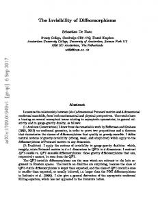
Algorithms for computing the group exponential of diffeomorphisms: performance evaluation∗ Matias Bossa Ernesto Zacur Salvador Olmos GTC, I3A, University of Zaragoza, Maria de Luna 1 (50018) Spain {bossa,zacur,olmos}@unizar.es
Abstract
sired because mappings must roughly preserve the smoothness of anatomical structures. The set of diffeomorphisms forms an infinite dimensional group with composition. A diffeomorphism ϕ(x) can be obtained as the end point of a flow φvt (x) defined by
In Computational Anatomy variability among medical images is encoded by a large deformation diffeomorphic mapping matching each instance with a template. The set of diffeomorphisms is usually endowed with a Riemannian manifold structure and parameterized by non-stationary velocity vector fields. An alternative parameterization based on stationary vector fields has been recently proposed, where paths of diffeomorphisms are the one-parameter subgroups, identified with the group exponential map. A LogEuclidean framework was proposed to compute statistics on finite dimensional Lie groups and later extended to diffeomorphisms. A fast algorithm based on the Scaling and Squaring (SS) method for the matrix exponential was applied to compute the exponential of diffeomorphisms. In this work we evaluate the performance of different approaches to compute the exponential in terms of accuracy and computational time. These approaches include forward Euler method, Taylor expansion, iterative composition, SS method, and a combination of interpolation and SS. In our results the SS method obtained the best performance tradeoff, as it is accurate, fast and robust, but it has an intrinsic lower bound in accuracy. This lower bound can be partially overcome by oversampling the grid, at the expense of increased memory and time requirements. The Taylor expansion provided a fast alternative when spatial frequencies are small, and particularly for low ambient dimensions, but its convergence is not guaranteed in general.
d v φ (x) = v(t, φvt (x)) dt t
with initial condition φv0 (x) = x, and v : [0, 1] → V a time-dependent velocity vector field, i.e. ϕ(x) ≡ φ1 (x). An inner product �v1 , v2 �V ≡ �Lv1 , Lv2 �L2 can be defined in the space of velocity vector fields v that endows C r with a Riemannian manifold structure. L is an invertible linear differential operator that guarantees the smoothness of v and therefore the smoothness and invertibility of ϕ(t). Distance between two diffeomorphisms can be measured with the length of the geodesic connecting them [8, 2]. In a recent work [1] the subset of diffeomorphisms obtained by constraining v to be a stationary vector field d v φ (x) = v(φvt (x)) dt t
(2)
was used to parameterize transformations between medical images. This parameterization showed a similar registration performance (accuracy and smoothness) than diffeomorphisms parameterized by non-stationary vector fields, with a significant computational complexity saving [7]. The paths of diffeomorphisms defined by (2) are identified with the one-parameter subgroups, and therefore with the group exponential map: exp(v) ≡ φv1 (x) = ϕv (x). Note that being a one-parameters subgroup implies φv2t (x) = φvt (x) ◦ φvt (x) = φvt (φvt (x)), and therefore exp(t v) = φvt (x) = ϕtv (x). Within this framework, the Log-Euclidean distance was defined as d(ϕ1 (x), ϕ2 (x)) = � log(ϕ1 ) − log(ϕ2 )�V ≡ �L log(ϕ1 ) − L log(ϕ2 )�L2 , being the group logarithm log(ϕ) = v(x) the inverse map of exp(v) ( from now on, we will drop the superscript v form φvt (x) and ϕv (x) ). Vector fields v(x) can be thought as vectors on a Hilbert space and
1. Introduction Computational Anatomy is a paradigm in which images are mapped to a template by means of large deformation diffeomorphic mappings [5]. A C r − diffeomorphism is an invertible map ϕ : Ω → Ω that is r times differentiable, where Ω is the image domain. The differentiability of ϕ(x) is de∗ This work was funded by research grants TEC2006-13966-C03-02 from CICYT, Spain
1
978-1-4244-2340-8/08/$25.00 ©2008 IEEE
(1)
standard Euclidean computation can be done with vectors Lv(x) [4]. Even though the metric linked to this distance is neither left- nor right-invariant, it provides a powerful framework where statistics can be more easily computed than in the Riemannian distance framework. In [1], the standard Scaling and Squaring (SS) and Inverse Scaling and Squaring (ISS) methods for computing the matrix exponential and logarithm respectively, was applied to compute the group exponential and logarithm of diffeomorphisms. In [4] the Baker-Campbell-Hausdorff (BCH) formula was applied in the diffeomorphism group. The BCH formula provides an expression for the logarithm of a composition of two exponentials v3 (x) = log(exp(v1 ) ◦ exp(v2 )) as a series expanded in terms of the Lie bracket [v1 (x), v2 (x)]. In this work, we analyzed various numerical schemes to compute the group exponential map, i.e. explicit forward Euler integration, Taylor expansion series, composition of small diffeomorphisms, SS and SS with v(x) interpolated at a finer grid. We compared performance of the methods in terms of accuracy and computational time for various experimental setting (i.e. ambient dimension 1, 2 and 3, amount of displacement and spatial frequency).
2. Numerical implementation of the group exponential of diffeomorphisms We discuss several methods to solve equation (2). In practice v(x) is obtained either as the outcome of an image registration procedure, or indirectly from an estimation of the logarithm. In both cases the data is sampled at a regular grid. Vector fields v(x) belong to a linear vector space, therefore any kernel interpolation scheme can be used, providing different degrees of smoothness. However, much more care must be taken when interpolating diffeomorphisms, which is essential in the composition operation. Diffeomorphisms must be invertible everywhere, and most interpolation schemes do not guarantee invertibility. Computing the interpolation that guarantees invertibility [6] is a task even more complex than solving (2). Given two sets of N nonN d coincident points {xi }N i , {yi }i ∈ R (in our case xi are the grid locations), this method finds a diffeomorphism such that yi = ϕ(xi ). In this work we tackle the problem of estimating the diffeomorphisms φt (x) at t = 1, solution of equation (2), given a stationary velocity vector field v(x) known at any point, defined by a known function or by the grid sampling together with an interpolation scheme, being the latter the most common situation in practical applications. We analyzed the case of grid sampling with (bi- tri-)linear interpolation because of its small complexity. This study could be extended to more complex interpolation schemes.
Forward Euler method. This basic integration method consists in dividing time in N small steps, and updating φt (x) as φt+dt (x) = φt (x) + dt v(φt (x)),
(3)
with φ0 (x) = x and dt = N1 . In practice, it is more accurate to update only the displacement field ∆t (x) ≡ φt (x) − x, i.e. ∆t+dt (x) = ∆t (x) + dt v(x + ∆t (x)), because the arguments of the sum have similar order of magnitude. Computational time increases linearly with the number of steps N , that can be arbitrarily large, providing arbitrary large accuracy limited by machine precision. We chose as our ground truth Forward Euler method because of the two following reasons: the accuracy can be controlled by the number of steps N , and secondly, interpolation is only performed on vector field v(x). Other methods require interpolation of diffeomorphisms, which is a more complex task and prone to error. Taylor expansion. The velocity vector field v can be writ�d ten as v(x) = i=1 vi (x)ei , where {ei }di=1 is an orthogonal basis of Rd . If the components vi (x) are analytic then the solution of Eq. (2) is also analytic, and is given by the formal power series [10] φt (x) = etV x =
∞ n � t n V x, n! n=0
(4)
�d ∂ where V ≡ i=1 vi (x) ∂xi is a differential operator and n V denotes the n-fold self-composition of V . The assumption of (bi- tri-) linear interpolation is in contradiction with the analiticity requirement of vi (x). However, in this work it is assumed that derivatives can be approximated by centered differences. Equation (4) is clearly a generalization of the Taylor expansion of the exponential of scalar numbers, and it is often known as Lie Series. The first terms of the expansion are given by v 0 (x) v 1 (x) v 2 (x) v 3 (x)
= x = v(x) � ∂v(x) = vi (x) ∂xi i � � � � ∂ ∂v(x) = vj (x) vi (x) ∂xj ∂xi j i .. .
The same result can be obtained by direct derivation of
starting with φ2−N (x) = x + 2−N v(x). The SS method is fast because only N composition are needed, while the composition and Euler methods require 2N steps for the same initial approximation. The main limitation of this method is that interpolation of possible highly nonlinear diffeomorphisms is performed in the last steps. Even though the approximation exp(v/2N ) ≈ x+v(x)/2N can be very accurate using large values of N , the sampling error made in the computation of the last squaring φ1 (x) = φ1/2 (φ1/2 (x)) may be large. Therefore, the SS method applied to diffeomorphisms has an intrinsic lower bound in accuracy, related to the interpolation scheme.
φt (x) with respect to time, and using Equation (2), φt (x)|t=0 d φt (x)|t=0 dt d2 φt (x)|t=0 dt2
= x = v(φt (x))|t=0 = v(x) d v(φt (x))|t=0 = dt � ∂v(x) d φt,i (x)|t=0 = = ∂xi dt i � ∂v(x) vi (x) = ∂xi i =
An advantage of the Taylor expansion is that no interpolation is required, the value of φt (x) at each point x is only determined by the derivatives of v(x) at that point. The method can be used to compute exactly a diffeomorphism of a known analytic v(x). Composition method. As φt (x) belongs to a oneparameter subgroup, φr+s (x) = φr (x) ◦ φs (x) = φs (x) ◦ φr (x) and φ0 (x) = x. In particular, if φ1/N (x) is known, then φ1 (x) = (φ1/N (x))N , (5) which can be iteratively computed as φt+dt (x) = φdt (x) ◦ φt (x)
(6)
where dt = 1/N . For small dt, φdt (x) can be approximated by x + dt v(x). This initialization generates the same analytical solution as the Euler method, as r.h.s. of (6) equals φt (x) + dt v(φt (x)) which is exactly the same as in (3). However the numerical implementation of both methods do not have the same performance because due to the limited machine precision, the computation of φdt (x) = x + dt v(x) at the first stage could introduce a significant error. In addition, even though the composition φdt (x) ◦ φt (x) = φt (x) ◦ φdt (x), their numerical implementations are quite different. While the left term is computed as φt (x) + dt v(φt (x)) where v(x) is linearly interpolated (according to our assumption), the right term is computed as φt (x + dt v(x)), and a possible large and highly non-linear φt (x) must be sampled. Linear interpolation was used because an appropiate interpolation is unknown, introducing larger errors. Scaling and Squaring method. This method is based on N the equality exp(v) = (exp(v/2N ))2 , and the assumption that exp(v/2N ) ≈ x + v(x)/2N for large N . Then exp(v) can be computed by recursive squaring N times exp(v/2N ) φ2t (x) = φt (x) ◦ φt (x) = φt (φt (x)),
(7)
Interpolated Scaling and Squaring method. In [3] the frequency behaviour of composition was analysed, and it was argued that the essentially band-limiting frequency of a scalar composition h(x) = g(f (x)) is given by νh = νg max |f � (x)|, where ν denotes the maximum frequency. Applying this rule to the composition d d (5), νφ1 = νv (max | dx φdt (x)|)N −1 = νv (max | dx (x + N →∞
d v(x)|/N )N −1 −−−−→ v(x)/N )|)N −1 ≈ νv (1 + max | dx d νv exp(max | dx v(x)|). Therefore, the spatial frequency of ϕ(x) exponentially scales with frequency and magnitude of v(x). The multidimensional case was also analyzed in [3], arriving to a similar band-limit. This suggests that for vector fields v(x) with either large magnitude or frequency, an upsampling would be required to avoid aliasing. In order to reduce the interpolation error of the SS method, we propose to interpolate v(x) in a finer grid than the original and then to apply the SS method. A big limitation of this method, is that the memory requirement is increased by a factor for r2d , being d the ambient dimension, and r the interpolation ratio of the grid.
3. Experiments and results Simulated experiments. Random vector fields were generated on isotropic regular grids of sizes 500, 100x100 and 60x60x60, for ambient dimensions 1, 2 and 3 respectively. In order to reduce boundary condition effects, a rectangular window was applied to cancel out the 10 outer samples, and a Gaussian smoothing of a variable σ was applied. Finally the velocity vector fields was scaled in order to obtain several displacement magnitudes. The accuracy of each estimation method was assessed by the RMS and maximum absolute value of the displacement field error, being the ground truth the forward Euler method with a time step of 0.001, i.e. N = 1000. Results of accuracy vs. computational time for a wide range of the free parameter in each method are illustrated in Fig. 1, 2 and 3 for 3D, 2D and 1D respectively. In the case of interpolated SS method, there are two free parameters:
1
0
Error (voxel size)
10
−1
10
−2
10
−3
−1
−1
10
−2
10
−4
0
1
10 Time (seg.)
10
−3
10
−1
0
10
1
10 Time (seg.)
10
−5
−1
0
10
1
10 Time (seg.)
10 −2 10
2
10
10
40
40
40
40
35
35
35
35
30
30
30
25
25
25
50
20 40
15 0 20
40
15 0
30
10
50
20
10 20
20
10 20
50
0
1
Error (voxel size)
−2
10
50
1
0
1
0
−1
0
10 Euler Taylor Composition SS SS Int.
10
10
20 10
40
0
10 Euler Taylor Composition SS SS Int.
10
−1
10
20 30
0
Error (voxel size)
0
10
30
10
20
50
10 Euler Taylor Composition SS SS Int.
50 40
0
10
40
1
10
2
10
20
30 10
40
1
10
15
30
Euler Taylor Composition SS SS Int.
0
10 Error (voxel size)
50
Error (voxel size)
0
30 10
40
0
10 Time (seg.)
25
40
20
30
−1
10
30
50
20 15
30
−3
10
−4
10 −2 10
2
10
−2
10
10
−5
10 −2 10
2
10
−2
10
10
−4
−1
10
Euler Taylor Composition SS SS Int.
−1
10
−4
10
10 −2 10
10 Euler Taylor Composition SS SS Int.
10
−3
10
0
10 Euler Taylor Composition SS SS Int. Error (voxel size)
0
10 Error (voxel size)
0
10 Euler Taylor Composition SS SS Int.
Error (voxel size)
1
10
−1
10
−2
10
−1
10
−2
10
−2
10
−3
−3
10
−4
−3
−1
0
10
1
10 Time (seg.)
−4
10 −2 10
2
10
10
−1
0
10
1
10 Time (seg.)
30
10
40
35
35
30
0
20
0 10 20
20
50
0
2
Error (voxel size)
0
10
−1
10
50 1
1
1
0
10
−1
10
0
10 Euler Taylor Composition SS SS Int.
10
10
10
40
2
10
20 30
10 Euler Taylor Composition SS SS Int. Error (voxel size)
1
20
0
0
3
10
30
10
20
50
2
40
0
10
40
10 Euler Taylor Composition SS SS Int.
50
20
30
10
40
10
2
10
15
30
30
10 50
40
15
30 20
30 40
1
10
50 40 10
20
0
10 Time (seg.)
25 50
20
30
−1
10
30
25
15
10
10 −2 10
2
10
40
20
0
1
10
35
40
15
0
10 Time (seg.)
25
50
20
−1
10
40
30
25
−4
10 −2 10
2
10
40 35
10
Euler Taylor Composition SS SS Int.
0
10 Error (voxel size)
10 −2 10
Error (voxel size)
−3
10
0
10
−1
10
−1
10
−2
−2
10
−2
10
10
−2
10
−3
−3
10 −2 10
−1
0
10
1
10 Time (seg.)
2
10
10
−3
10 −2 10
−1
0
10
1
10 Time (seg.)
−3
10 −2 10
2
10
10
−1
0
10
1
10 Time (seg.)
10 −2 10
2
10
10
40
40
40
40
35
35
35
35
30
30
30
25
25 50
20 40
15 0
30
10 20 30 10
40 50 60
0
0
1
10 Time (seg.)
2
10
10
30
25
25 50
20
50
20
50
20 40
15 0
30
10 20
−1
10
20
20 30 10
40 50
40
15 0
30
10 20
20 30
0
30
10 20
20 30
10
40 50
0
40
15
0
10
40 50
0
Figure 1. Odd rows: accuracy vs CPU time for the estimation of the exponential of a 3D vector field. Maximum (RMS) error is plotted with solid (dotted) lines. Even rows: illustration of the corresponding deformation grid at mid slice. Increasing displacement magnitudes from top to bottom. Decreasing σ of the Gaussian smoothing from left to right.
1
1
10
10 Euler Taylor Composition SS SS Int.
0
Error (pixel size)
10
−1
10
Euler Taylor Composition SS SS Int.
−1
10 Error (pixel size)
0
10 Error (pixel size)
0
10 Euler Taylor Composition SS SS Int.
−1
10
−2
10
−2
10
−3
10
−2
10
−3
−4
10
−3
10
10
−4
−3
10
−2
10
−1
10 Time (seg.)
0
10
10
1
10
−5
−3
10
4
−2
10
−1
10 Time (seg.)
0
10
1
10
10
1
10
3
10
−2
10
−1
10 Time (seg.)
0
10
1
10
1
10 Euler Taylor Composition SS SS Int.
−3
10
10 Euler Taylor Composition SS SS Int.
0
10
Euler Taylor Composition SS SS Int.
0
10
1
10
0
10
Error (pixel size)
Error (pixel size)
Error (pixel size)
2
10
−1
10
−1
10
−2
10
−2
10
−3
10
−1
10
−2
10
−3
−3
10
−2
10
−1
10 Time (seg.)
0
10
1
10
10
−4
−3
10
−2
10
−1
10 Time (seg.)
0
10
Figure 2. Idem Fig. 1 for 2D.
1
10
10
−3
10
−2
10
−1
10 Time (seg.)
0
10
1
10
1
Euler Taylor Composition SS SS Int.
0
−1
10
−2
10
−3
10
−1
10
−2
10
−3
10
−4
10
10
−4
−5
−4
−4
−3
10
−2
10
10
−1
10
10
−4
−3
10
−2
10
Time (seg.)
50
100
150
200
250
−4
−3
10
10
10 0 −10 0
10
−1
10
−2
10
300
350
400
450
1
50
100
150
200
250
300
350
400
450
0
1
Euler Taylor Composition SS SS Int.
Euler Taylor Composition SS SS Int.
0
−2
100
150
200
250
300
350
400
450
Euler Taylor Composition SS SS Int.
−1
10
Error (grid size)
Error (grid size)
−1
50
10
10
10
10
0
10
0
0
10
10 0 −10 0
10
10
−1
10 Time (seg.)
Time (seg.)
10 0 −10
Error (grid size)
−2
10
−3
10
Euler Taylor Composition SS SS Int.
−1
Error (grid size)
10
Error (grid size)
10
Error (grid size)
10
10 Euler Taylor Composition SS SS Int.
0
10
0
1
10
−1
10
−2
10
−3
10
−2
10
10
−4
10
−3
10
−3
−4
−3
10
−2
10
10
−1
10
10
−5
−4
−3
10
−2
10
Time (seg.) 10 0 −10
10
50
100
150
200
250
300
350
400
450
3
100
150
200
250
300
350
400
450
0
1
Error (grid size)
10
1
10
0
10
−1
0
10
−1
10
−3
−2
10
10
−1
10
10
100
150
200
250
300
400
450
300
350
400
450
Euler Taylor Composition SS SS Int.
−1
10
−2
10
−3
−2
10
10
−1
10
−4
−3
10
10
−2
10
−1
10 Time (seg.)
Time (seg.)
350
250
−4
−4
10 10 0 −10
50
200
−3
Time (seg.) 10 0 −10 0
150
10
−3
−4
100
0
10
−2
50
10
−2
10
−1
10
10 Euler Taylor Composition SS SS Int.
Error (grid size)
2
−2
10
1
2
10
Error (grid size)
50
10 Euler Taylor Composition SS SS Grid
10
−3
10
10 0 −10 0
10
10
−4
10
Time (seg.)
10 0 −10 0
10
−1
10 Time (seg.)
0
10
10
10 0 −10 0
50
100
150
200
250
300
350
400
450
0
50
100
150
200
250
300
350
400
450
Figure 3. Idem Fig. 1 for 1D, except for displacement functions ϕ(x) − x in even rows.
N and the interpolation ratio. In our experiments N was set to 7 and the interpolation ratio ran from 1 to 6 at least. Computations were performed using a 1.83GHz Core 2 Duo processor within a 2GB memory standard computer running Matlab under Linux. Linear interpolation was implemented as C source mex files. Exponentials of intersubject 3D brain mappings. In order to illustrate the performance in a more realistic case, such as the atlas estimation from a set of 3D brain T1 MRI images, we computed exponentials of vector fields characterizing intersubject mappings. A subset of 23 images was selected from LPBA40 database from LONI UCLA [9]. An image was randomly selected as template and diffeomorphic non-rigid registration [7] was performed to the remain-
ing 22 cases. The outcome of this algorithm is a vector field v(x). The results of the error in the estimation of the exponentials are shown in Fig. 4.
4. Discussion Explicit forward Euler. Its performance was robust for the range of spatial frequencies and displacements magnitudes. Taylor expansion. Looking at the results, two main problems of the Taylor expansion can be highlighted. Firstly, it diverged at high displacement magnitudes, for example in the bottom row of Figures 1-3. Secondly, the best accuracy was obtained with an expansion order that decreased for higher spatial frequencies. This behaviour is more clearly
4
8
10
10 Euler Taylor Composition SS SS Grid
3
10
2
6
10
1
10
N
Error (voxel size)
10
Composition SS
4
10
0
10
−1
10
2
10 −2
10
−3
10
0
0
10
1
2
10
10
3
10
Time (seg.)
Figure 4. Error (mean ± standard deviation) vs CPU time in the estimation of exponentials of 3D vector fields from intersubject brain registration. Maximum (RMS) error is plotted with solid (dotted) lines.
10
0
0.5
1
1.5
Error (voxel size)
Figure 6. Complementary cumulative histogram of the error for composition and SS method. Curves with different values of N : from top-right to bottom-left corner, N = 5, 10, 15, 20, 25, 30 for Composition and N = 2, 3, 4, 5, 6, 7 for SS method.
Composition. As it was previously mentioned in Section 2, the accuracy of the composition method was systematically worst than forward Euler method, except for 3D large deformations (regardless of the spatial frequency), where it performs almost equal to the Euler method (see bottom row of Fig. 1). Scaling and Squaring. This method provided the best accuracy-time trade-off for most of the situations. The main drawback is that it showed an accuracy bound, i.e. large values of N did not improve accuracy. The bound was usually reached with N about 7-10 for most situations (ambient dimension, displacement magnitude and spatial frequency). The worst performance was obtained at large deformations and spatial frequencies.
Figure 5. Illustration of deformation grids superimposed on brain images. Left: source image and forward mapping. Right: target image and inverse mapping.
Scaling and Squaring with interpolation. This method allowed to obtain better accuracy than the SS method at the expense of bigger computational requirements, both in memory and time. In particular, for 1D, it was the fastest method among the most accurate methods.
seen in top row of Figures 2 and 3. The reason is that high order expansion terms do not contribute effectively to improve the accuracy because derivatives are estimated by simple centered finite differences, with more emphasis at high spatial frequencies. In contrast, at 1D Taylor expansion method outperformed the others methods in speed (look at the 4 panels closer to top-left corner in Fig. 3).
All in all, it can be said that the SS method with N ≈ 8 is a good choice for an RMS error of about some hundredths of voxel size. In some situations, the maximum error may reach voxel size. If better accuracy is required in 3D, the forward Euler method should be used at high spatial frequencies (see right columns of Fig. 1). In the special case of small and medium deformations and frequency in 1D (see the 4 panels closer to top-left corner in Fig. 3), the Taylor expansion method provided similar accuracy with less computational time.
3D MRI brain images. In a realistic intersubject brain registration application, the best performances was obtained by the SS method (see Fig. 4). Note that the performance variability in the 22 subjects was small compared to the performance difference among methods. A small accuracy gain, with a different method, would require a high increase of time. It can be appreciated a dramatic error rise for the SS method at N ≈ 13. This behaviour is because machine precision was insufficient to compute x + v(x)/2N . While in the simulated experiments section double precision was used, in this case computations were done with single precision due to memory issues. If double precision were used, the same error-time curve would be obtained up to N ≈ 13, appearing the error rise at N ≈ 40. Fig. 5 shows an example of intersubject brain registration illustrating the order of magnitude of spatial frequencies as well as deformation magnitudes typically found. In order to get a better insight into the distribution of the error complementary cumulative histograms, i.e. the number of voxels with error larger than a given value, are shown in Fig. 6. It is clearly seen that the number of voxel with very large errors in the SS method is much lower that in composition method. These large errors for the SS method where mostly located around the lateral ventricles.
5. Conclusions The performance of several methods to compute the group exponential of diffeomorphisms was analyzed in this paper. Among these methods, a variation of the Scaling and Squaring method was proposed, that slightly increased the accuracy at the expense of an increase of time and memory requirements. In our two experiments, including simulated data and brain data sets, the SS method obtained the best accuracytime trade-off. However, a lower bound in accuracy was found, normally reached with N about 8 to 10. All the experiments were performed using (bi-tri) linear interpolation. Error-time curves could be very different with an alternative interpolation scheme, although the lower bound in accuracy of the SS method would remain. The Taylor expansion approximation would probably be the most sensitive to the interpolation scheme. For 1D applications, such as histogram analysis or time series warping and analysis, or in the cases of very low spatial frequency, the Taylor expansion method with a small number of terms can be an efficient option. It must be kept in mind that in diffeomorphic registration applications the spectrum of spatial frequencies of v(x) depends on the regularizer imposed in the optimization algorithm. The performance analysis on a wide range of situations (ambient dimensions, deformation amplitudes and spatial frequencies) done in this work provides useful information to select the best free parameter and method to
compute the group exponential of vector fields. In particular, in a multiscale registration it may be sensible to use different degrees of regularization at each scale. An advantage common to forward Euler and Taylor expansion method is that the diffeomorphisms can be computed on isolated points as well as on non-uniform grids, with a computational load proportional to the number of points. In contrast, in the SS and composition methods a sampling of the whole domain is used.
References [1] V. Arsigny, O. Commonwick, X. Pennec, and N. Ayache. Statistics on diffeomorphisms in a Log-Euclidean framework. MICCAI, 4190:924 – 931, 2006. [2] M. F. Beg, M. I. Miller, A. Trouve, and L. Younes. Computing large deformation metric mappings via geodesic flows of diffeomorphisms. IJCV, 61 (2):139–157, 2005. [3] S. Bergner, T. Moller, D. Weiskopf, and D. J. Muraki. A spectral analysis of function composition and its implications for sampling in direct volume visualization. IEEE Transactions on Visualization and Computer Graphics, 12(5):1353– 1360, 2006. [4] M. Bossa, M. Hernandez, and S. Olmos. Contributions to 3d diffeomorphic atlas estimation: Application to brain images. In MICCAI, pages 667–674, 2007. [5] U. Grenander and M. I. Miller. Computational anatomy: an emerging discipline. Q. Appl. Math., LVI(4):617–694, 1998. [6] H. Guo, A. Rangarajan, and S. Joshi. Diffeomorphic point matching. The Handbook of Mathematical Models in Computer Vision, 2005. [7] M. Hernandez, M. N. Bossa, and S. Olmos. Registration of anatomical images using geodesic paths of diffeomorphisms parameterized with stationary vector fields. In MMBIA Workshop at ICCV, pages 1–8, 2007. [8] M. I. Miller, A. Trouve, and L. Younes. On the metrics and Euler-Lagrange equations of computational anatomy. Ann. Rev. Biomed. Eng, 4:375–405, 2002. [9] D. W. Shattuck, M. Mirza, V. Adisetiyo, C. Hojatkashani, G. Salamon, K. L. Narr, R. A. Poldrack, R. M. Bilder, and A. W. Toga. Construction of a 3d probabilistic atlas of human cortical structures. NeuroImage, 39(3):1064–1080, 2008. [10] R. Winkel. An exponential formula for polynomial vector fields. Advances in Mathematics, 128(1):190–216, 1997.