16 Oct 2004 - Dror [13] collected a significant number of applications of CARP variants and of corresponding solution ...... Local search with perturbations for the prize- collecting steiner tree problem in graphs. Networks, 38:50â58, 2001.
Algorithms for large directed CARP instances: urban solid waste collection operational support
Vittorio Maniezzo
Technical Report UBLCS-2004-16 October, 2004
Department of Computer Science University of Bologna Mura Anteo Zamboni 7 40127 Bologna (Italy)
The University of Bologna Department of Computer Science Research Technical Reports are available in PDF and gzipped PostScript formats via anonymous FTP from the area ftp.cs.unibo.it:/pub/TR/UBLCS or via WWW at URL http://www.cs.unibo.it/. Plain-text abstracts organized by year are available in the directory ABSTRACTS.
Recent Titles from the UBLCS Technical Report Series 2003-15 Gossip-based Unstructured Overlay Networks: An Experimental Evaluation, Jelasity, M., Guerraoui, R., Kermarrec, A-M., van Steen, M., December 2003. 2003-16 Robust Aggregation Protocols for Large-Scale Overlay Networks, Montresor, A., Jelasity, M., Babaoglu, O., December 2003. 2004-1 A Reliable Protocol for Synchronous Rendezvous (Note), Wischik, L., Wischik, D., February 2004. 2004-2 Design and evaluation of a migration-based architecture for massively populated Internet Games, Gardenghi, L., Pifferi, S., D’Angelo, G., March 2004. 2004-3 Security, Probability and Priority in the tuple-space Coordination Model (Ph.D. Thesis), Lucchi, R., March 2004. 2004-4 A New Graph-theoretic Approach to Clustering, with Applications to Computer Vision (Ph.D Thesis), Pavan., M., March 2004. 2004-5 Knowledge Management of Formal Mathematics and Interactive Theorem Proving (Ph.D. Thesis), Sacerdoti Coen, C., March 2004. 2004-6 An architecture for Content Distribution Internetworking (Ph.D. Thesis), Turrini, E., March 2004. 2004-7 T-Man: Fast Gossip-based Construction of Large-Scale Overlay Topologies, Jelasity, M., Babaoglu, O., May 2004. 2004-8 A Robust Protocol for Building Superpeer Overlay Topologies, Montresor, A., May 2004. 2004-9 A Unified Approach to Structured, Semistructured and Unstructured Data, Magnani, M., Montesi, D., May 2004. 2004-10 Exact Methods Based on Node Routing Formulations for Arc Routing Problems, Baldacci, R., Maniezzo, V., May 2004. 2004-11 Mapping XQuery to Algebraic Expressions, Magnani, M., Montesi, D., June 2004. 2004-12 VDE: Virtual Distributed Ethernet,Davoli, R., June 2004. 2004-13 SchemaPath: Extending XML Schema for Co-Constraints, Marinelli, P., Sacerdoti Coen, C., Vitali, F., June 2004. 2004-14 Intelligent Web Servers as Agents, Gaspari, M., Dragoni, N., Guidi, D., July 2004. 2004-15 SIR: a Model of Social Reputation, Mezzetti, N., October 2004.
Algorithms for large directed CARP instances: urban solid waste collection operational support Vittorio Maniezzo3
Technical Report UBLCS-2004-16 October, 2004 Abstract Solid waste collection in urban areas is a central topic for local environmental agencies. The operational problem, the definition of collection routes given the vehicle fleet, can greatly benefit of computerized support already for medium sized town. While the operational constraints can greatly vary, the core problem can be identified as a capacitated arc routing problem on large directed graphs (DCARP). This paper reports about the effectiveness of different metaheuristics on large DCARP instances derived from real-world applications.
. Department of Computer Science, University of Bologna, Mura Anteo Zamboni, 7 40127 Bologna, Italy.
1
1 Introduction
1
Introduction
The widely acknowledged increase in solid waste production, together with the increased concern about environmental issues, have led local governments and agencies to devote resources to solid waste collection policy planning. The problem, difficult per se, is further complicated by differential collection and recycling policies: this all leads to scenarios where manual planning of waste collection can easily yield severely inefficient solutions. It is known in fact that an efficient planning can have a significant impact on the overall costs of solid waste collection logistics [4]. Waste collection, as most logistic activities, can be studied at different levels: strategical, tactical, operational. In this work we concentrate on tactical planning, where a vehicle fleet and the service demand are given and the objective is to design the vehicle trips in order to minimize operational costs subject to service constraints. Specifically, this work derives from an experience of decision support for the waste collection sectors of municipalities of towns with about 100 000 inhabitants, with the objective of designing vehicle collection routes subject to a number of operational constraints. The reported results are for an abstraction level which does not consider several very specific issues, such as union agreements, third-party or personal contracts, etc. The problem to solve is modeled as a Capacitated Arc Routing Problem (CARP) on a directed graph and solved accordingly. Two main issues arose: CARP optimization. The instances to be solved are far bigger than the state of the art ones. Original heuristic approaches had to be designed in order to meet the solution quality and the allowed computation time specifications. Operator interface. It was needed to produce a system interface which could be effectively used by a service operator allowing him to fully understand problem instance and solution details, together with any manual intervention desired. While the second issue is of minor concern in this exposition, and the relevant GIS-based interface will only be sketched at the end of the work, the optimization issue will be detailed. The reported results have a relevance beyond the specific application, as several activities of realworld relevance can be modeled as CARP, foremost among them are mail collection or delivery, snow removal, street sweeping. The CARP is in fact a powerful problem model, which was originally proposed by Golden and Wong [16], and which, given its actual interest, have then been studied by many researches. Dror [13] collected a significant number of applications of CARP variants and of corresponding solution methodologies. For a survey the reader is also referred to [2]. In the literature, several heuristic approaches have been proposed for the CARP, while the only exact techniques so far were published by Hirabayashi et al. [20], who proposed a Branch and Bound algorithm and by Baldacci and Maniezzo [3], who transformed CARP instances into CVRP equivalents and proceeded solving these last. Moreover, Belenguer and Benavent [5] proposed an effective lower bound. However, being CARP NP-hard, exact techniques can seldom cope with the dimension of realworld instances. These call for heuristic and metaheuristic approaches: among the most recent proposals we remind the tabu search of Belenguer et al. [6], the tabu search of Hertz et al. [17], the VND of the same authors [18] (which will be detailed in Section 2.3) and the genetic algorithm of Lacomme et al. [21]. For a recent review, see [19]. As for more real-world oriented researches, we remind the work of Amberg et al. [1], who studied the M-CARP, that is a multidepot CARP with heterogeneous vehicle fleet, by means of a tabu search, of Xin [29], who implemented a decision support system for waste collection in rural areas based on UBLCS-2004-16
2
2 Urban solid state waste collection a simple Augment-Merge heuristic, of Snizek et al. [28] dealing with urban solid waste collection and of Bodin and Levy [8]. The general strategy adopted in this work is that of translating CARP into node routing problem instances and then study solution methodologies for the resulting data. Different approaches were compared, both directly applied to CARP data and to node routing translations. Among those, the most effective one is based on data perturbation [11] coupled with Variable Neighborhood Search and acting on a node routing problem reformulation. The paper is structured as follows. Chapter 2 introduces the problem of urban solid state waste collection, its reduction to directed CARP and two recent well-known heuristics for CARP. Chapter 3 presents the methodology we used, first transforming DCARP into ACVRP instances, then applying three variants of VNS to the resulting instances. Chapter 4 reports about the computational results we obtained, both on standard CARP testsets and on DCARP instances derived from real-world applications. Finally, Section 5 contains the conclusions of this work.
2
Urban solid state waste collection
The problem is defined over the road network of the town to support. The network is used as a basis for geocoding all problem elements, which are: one or more depots, where vehicles are stationed; landfills and disposal plants, where waste has to be brought, waste bins, which are usually specialized for differential collections. In our examples, we had the following waste types: 1. 2. 3. 4. 5.
undifferentiated; plastics; glass; paper; biologic or organic.
A number of vehicles are available, where each vehicle can load only bins of given types and has a capacity specified as a maximum number of bins. The actual problem faced asks for designing the routes of the available vehicles, in order to collect all specified bins, satisfying capacity and bin compatibility constraints, forbidding partial bin collection, with the objective of minimizing the total travel distance. Moreover, bins can be collected only within given time widows. Bins are set in an urban context, which can be modeled by means of a directed graph. One way streets and forbidden turns have to be considered. Each bin is moreover set on one specific side of the street. A vehicle driving along a street can usually collect all bins of a compatible type on the right side of that street. In case of one-way streets, the vehicle can instead collect both bins on the right and on the left side of the street, if adequately equipped. Figure 1 hints at some issues of urban bin collection when modeled on a graph. This work reports about an optimization procedure and a support system for an abstract version of the general problem, in that we consider only one depot and one disposal facility per waste type. Moreover, time windows are not considered and the number of vehicle is an input parameter and not UBLCS-2004-16
3
2 Urban solid state waste collection
3
8
C
ONE-WAY B 7 1
2
A
4
D
5
6
Figure 1. Conversion of a road network into a graph. Bin can be emptied only by a vehicle which travels the directed arc ������� � . Bin can be emptied only by a vehicle which travels the directed arc ����� �� . A vehicle travelling along the one-way arc ��������� can empty both bin � and � . a decision variable, thus the objective function is only given by the total distance traveled. However, the extension to actual settings is a lesser effort when compared to the ability of solving the core problem for actual dimension. This problem can be formulated as an extension of a well known problem from the literature: the Capacitated Arc Routing Problem (CARP). 2.1
Capacitated Arc Routing Problem
CARP was originally proposed by Golden and Wong [16] and is usually studied in a version which would correspond to an instance of the waste collection problem with a single depot, a single disposal unit coincident with the depot, only one bin type, a non-heterogeneous fleet and no temporal constraints. Moreover, the graph is undirected and bins are positioned on an arc, not on one side of an arc. Different mathematical formulations have been proposed for this version of the CARP ([16],[5], [2]), all of them for the undirected case. The problem we have to solve is however characterized by the fact that the road network of interest must be modeled as a directed graph, thus the problem to solve is a directed CARP (DCARP). We can take advantage of this in the mathematical formulation of the problem. Accepting the usual assumptions made for the formulation of the Vehicle Routing Problem (a problem very closely related to CARP, see section 2.2), a formulation of the DCARP can be the following one. Given: ���� � �
���������
the weighted digraph of interest;
set of vertices (nodes), where node 0 corresponds to the depot; set of arcs;
UBLCS-2004-16
4
2 Urban solid state waste collection
��� set of mandatory arcs (clients to service, arcs with bins); �� � set of vertices containing the endpoints of the arcs in and the depot; �� �� �� set of available vehicles, each of capacity � ; ���� � cost of arc ���� �� ; �� � � request associated with arc ���� �� �
�
�
�
���
�
� �
�
� �
�
� � ������� !� ���� �� � �! ��� � �� #" � �
�
assuming each arc �
�
to be connected, it is possible to transform it into a complete graph has a cost defined as follows:
��� � ��$ � � � % %& !� ' ( ����!� *���� )+�(-,�� .0/+1��!'0. �
�
$ �
�� �$
���
� ���
where
� �
�
& �!' ( ����
�
� $ � �
�
����
� �
� �
� �
2,43
being the cost of the shortest path in � from to . Note that the cost of a mandatory arc � �� can be considered both explicitly and implicitly, if the arc is part of a minimum cost path. The use of such a path would imply deadheading over � �� . The decision variables are defined as: � �
2,43
54� � 6 7� �
���� of $ � )+(-,�.0/+1��!'0. �
if arc
�
� �
is traversed by vehicle k
A three-indices formulation is as follows.
8+9;:=< �?> A@ C� BED ��$ � � D 54� � 6 F � �HGCIJ< 60IJK 'J (L M60D IJK 54� � 6 5�R!� 6 �S �#S ��D IPO0Q 60D IJK � � � 54� � 6UT � F � D�HGCI � 54� � 6 D 5W�H�X6 ��D IPO0Q ��IPO0Q D��I[Z �JD I[\ Z 54� � 6U] ��D IPO 5_^L� 6 54� � 6 � � � d �
�
(1)
���� N�
�
� �
�
�
� �
UBLCS-2004-16
(2) (3)
3V� �
�Y� �� 3V� � �` � ��a" � � 3b� � c, � ` ���� �� 3V� � �
�
�
�
� �
�
�
(4) (5) (6) (7) 5
2 Urban solid state waste collection The objective function (1) asks to minimize the total travel cost under the constraints that: each mandatory arc is serviced by exactly one vehicle (2, note however that each mandatory arc can be utilized by more than vehicles if it happens to be on the shortest path from an endpoint of a mandatory arc to that of another mandatory arc: only one vehicle will service it, though), the number of vehicles used is the number of available vehicles (3) and the capacity of each vehicle is not exceeded (4). Moreover, equalities (5) are continuity constraints, inequalities (6) are subtour elimination and constraints (7) are integrality constraints. 2.2
Transformation into an ACVRP
The huge dimension of the graphs we had to deal with, rules out the possibility to apply both exact methods and sophisticated heuristics. Our approach for solving the DCARP instances is based on their transformation into ACVRP (Asymmetric Capacitated Vehicle Routing Problem) instances. CARP and CVRP are in fact closely related, the main difference being that in the CARP clients are set on arcs while in the CVRP clients are set on the nodes. The CVRP has been more thoroughly studied in the literature and, even though instances of our size are still far from current state of the art, efficient heuristics are available for instances bigger than the CARP ones. The possibility to transform a CARP instance into a CVRP one is well-known, having been first proposed in the literature by Pearn et al. [25]. This transformation, when applied to a CARP defined on a graph with mandatory edges, results in a CVRP with 3 + 1 nodes. More recently, Baldacci and Maniezzo [3] presented an alternative transformation which results in a CVRP with 2 + 1 nodes. This transformation is of general validity, however, we can take advantage of the need to work on digraphs and use a modified approach which transforms a DCARP instance in an ACVRP one, by simply associating with each DCARP mandatory arc an ACVRP node which inherits the arc demand, by maintaining the depot node, and by redefining distances according to the formulation of section 2.1. Specifically, we compute the all pairs shortest paths matrix among every outgoing vertex , including depot node , and every incoming vertex , including depot node , for each � � � � ��� . We then add the cost , � � , to the cost � � of each path exiting from j. This results in a graph with + 1 nodes and � � �� � arcs, which defines an instance of ACVRP having the solution set which can be mapped 1 to 1 into equivalent DCARP solutions. In the case of our application the transformation function parses a DCARP instance and rewrites it as an equivalent ACVRP instance having:
@
@
@
�� � �
���� U� @
& �!' ( �, ���
@
�
���� 2, ��
�
- the same vehicle set with the same capacity constraints. - the objective function defined over the cost matrix as computed above. - multiple routes per vehicle, where the first one starts from the depot and ends at the disposal, all other ones start and end at the disposal except for the last one, which starts at the disposal and ends at the depot. - vehicle objections associated to each client: clients associated to nodes corresponding to twoways roads can be serviced by any vehicle, while clients associated to nodes corresponding to one-way roads can be serviced only by vehicles which can load bins both from their left and from their right side. Figure 2 shows the transformation on a simple graph. Since the ACVRP graph has a number of nodes corresponding to the number of clients of the DCARP instance, in the waste collection case we get a smaller graph than the original road network. UBLCS-2004-16
6
2 Urban solid state waste collection
1
1,2
2
3 4
3,7
5
4,8
6
7
8
0
0 10
9
10,11
11
Figure 2. CARP CVRP. a) DCARP graph. b) ACVRP graph (all edges are pairs of arcs).
The computational complexity is not determined by the road network graph, but by the number of clients. 2.3
Algorithms CARPET and VND-CARP
This subsection introduces two algorithms for the undirected CARP proposed by Hertz, Laporte and Mittaz, which represent the state of the art of the heuristics working directly on the CARP graph. The first one, called CARPET [17], is a Tabu Search like heuristic, the second one, called VND-CARP [18], is a Variable Neighborhood Descent. 2.3.1 CARPET CARPET is based on seven basic procedures: for their description we use the same notation as in [17], where � �� are vehicle routes, � �� are solutions, is the set of clients to service and �� is a generic client subset.
` ` 5 5 ?�� SHORTEN( ` ; `�� ). Given an input route ` which services a subset �� of clients the procedure returns, ` � which services the same clients �� but it is shorter. The implementawhen possible, a route � tion is involved —it is not completely specified even in [17]— but it is based on servicing in `�� the clients using a different ordering than in ` . `� a route ` which services a subset �� of clients and given a client (arc DROP( ` , (� � �� 6 ) � � � �� 6 ), DROP). Given returns a route which services �� " � � � �� 6 . ` � ). Given a route ` which services a subset �� of clients ADD constructs a route �` � ADD( ` , (� � �� 6 ) � which services the clients ��� � � � �� 6 . PASTE(5 ; ` ). Given a solution 5 consisting of @ routes, PASTE concatenates them so to obtain a single route ` � , to be processed by SHORTEN. CUT( ` , � , 5 ). This is another complex procedure, the general idea is to take in input a route ` servicing the clients in � , possibly exceeding the capacity constraints of the vehicle associated to ` , and to partition ` into routes each of which satisfies the capacity constraint. �
�
�
�
�
�
�
�
�
UBLCS-2004-16
�
�
7
2 Urban solid state waste collection
`
`
`
#�
SWITCH( , � ; � ). Given a route where a vertex � � appears more than once, this procedure computes an equivalent route �� where all subroutes having � as endpoints are travelled in the opposite direction than in .
`
5 5
`
5
POSTOP( ; ). Given a solution , this procedure tries to obtain another lower cost solution applying PASTE, SWITCH, CUT, SHORTEN.
5
by
`
For details, we refer the reader to [17] An initial solution for the tabu search is obtained by means of an heuristic for the Rural Postman Problem proposed by Frederickson [14]: where the Rural Postman Problem is a special case of the CARP where there are no capacity constraints and only one vehicle is available to build only one route. A CARP feasible solution can then be obtained by means of procedure CUT. Algorithm CARPET tries to minimize two functions: the cost function and a penalty function measuring the sum, over all vehicles, of the loads exceeding vehicle capacity. � The neighborhood set � � of a solution is obtained considering all pairs of routes , �� and all arcs � � ��� � serviced in . If � contains either only the depot or an arc having an endpoint which is far from � or � at least � (where � is a parameter), the a neighbor is obtained invoking DROP( , and �� with and �� , respectively. (� ��� ) ) and ADD( �� , (� ��� ) �� ) and replacing in the solution � The tabu list is computed as follows. If is feasible and its best neighbor � � � is not better then , then a try is made to improve by invoking ADD and DROP on each arc corresponding to a client in . Each time an arc is removed from a route it is declared to be tabu for � iterations (where � is randomly chosen in the interval � � � � �� ). Various other parameters are dynamically updated during a run. For details, see [17].
5
� 6 � � 6 `
6
`
`
5
5
5
`
� 6 `
5 `
5
5
` `
`
�
`
5 �
`
5
`
`
2.3.2 VND-CARP VND-CARP is a Variable Neighborhood Descent algorithm [18], defined as follows. � � - The first neighborhood function � � is defined moving an arc � � ��� � associated with a client fro a route to another route �� which —as in the case of CARPET— either contains only the depot or contains another arc associated with a client and having an endpoint sufficiently far from either � or � . � - A neighbor � � is obtained by modifying routes of as follows: the routes of are concatenated to make a single route (such as in PASTE of CARPET). The is divided by CUT, creating new feasible routes and a new solution �� , which is finally improved by SHORTEN. For details, see [18].
`
�
�5
5
`
6
�
� 6
`
5
5
`�
5
This algorithm makes use of 5 of the 7 procedures introduced for CARPET [18], SHORTEN, SWITCH, ADD, DROP, CUT, and of the Frederickson algorithm [14] to generate an initial solution, which is made feasible by the CUT. As a final remark, notice that, since it is computationally infeasible to compute the best neighbor � in � � , the choice is made for the best neighbor among a restricted set of randomly generated ��
neighbors, � ��� � � � . In [18]
�� , where
is the sum of all clients weights and is the vehicle capacity.
�5
�
�
VND-CARP ��� 1 Compute an initial solution ��
� 2
�� , �
�
d� 5 A5
UBLCS-2004-16
�
d�
� �
�
5 8
3 New metaheuristics 3 4 5 6 7 8 9 10 11 12 13 14 15 16 17 18 19
�
�
5
/*counter of the number of neighborhoods*/ � � /*cost of best neighbor*/ Select routes, apply SWITCH and CUT Apply SHORTEN to each new route. The new solution is �� if � � � �� � � �� � � � �� then � � �
�
�
�
2 5 5 A5 � A�� � if � T � � then goto 4 � A 5 if � 5 5 �
5
5
�
�
�
then � � � goto 3 i = i-1 if � then goto 3 � � � if � �� then goto 2 else return �
�]
5 A 5
5
5
The algorithm returns � as the best found solution.
3
New metaheuristics
Unfortunately, the size of the ACVRP instances of interest for us are very big (hundreds or thousands of nodes) thus all but very simple heuristics are ruled out. We implemented three such heuristics; all of them make use of a local search procedure based on the following neighborhoods: 1. move of a client within one same route. 2. move of a client from a route to another. 3. swap of two clients within one same route. 4. swap of two clients of different routes. 5. 3-opt within one same route. 6. single point route crossover [21]. The basic approach we used for solving the ACVRP instances was a modified Iterated Variable Neighborhood Search. Variable Neighborhood Search (VNS) is an approach proposed by Mladenovi´c and Hansen [24], whose basic framework is the following:
JB?�C( � �� 8 [( � )+B
VARIABLE N EIGHBORHOOD S EARCH ��� 1 ��� �� � � � 2 Define the set of neighborhood structures to be used during search 3 Generate an initial solution 4 repeat UBLCS-2004-16
5
6 3 �
�
3 ��
���
�
9
3 New metaheuristics
3
5 6 7 8 9 10 11 12 13 14 15 16 17
� �
` , �W3P�CB
repeat �
�
�
5
3
Randomly generate a solution �� in the -th � neighborhood of , � � �
5 5 � 6 5
3 � Y) � 2'0. �[/ � , Find the local optimum 5�� using neighborhood 3_ if 5 � is better than 5 then 5 A5 � 3 � else 3 3 until 3 �
3 �� until �(!.0/ @ �CB �[( � )+B � )+B & �C( � )+B �
�
���
�
�
� �
�
�
�
�
` , W3P�CB
Notice that the � � at line 7 implements a search diversification which permits to escape form cyclic dynamics. The way shaking is implemented deeply affects the algorithm performance. We implemented three different shaking strategies: random multistart, a genetic algorithm and data perturbation. Before describing the three variants, we present the initial solution construction procedure, which is common to the three of them. To construct initial solutions we used a two phase algorithm [10] because it is fast and consistently produces solutions of reasonable quality. 3.0.3 Two Phase construction algorithm The two phase algorithm [10], constructs a solution in two different ways, one per phase, starting from the same pivots. We remind that a ��� � �� is the first client assigned to a vehicle, its proper choice is essential for the construction of a good route as it determines the area where the vehicle will operate. Usually, pivots are chosen as the customers hardest to service, therefore nodes which have high requests, which are far from the depot, which are far from previously considered routes, etc. The two phases share only the pivot set and are otherwise independent from one another. The solution proposed is the best among the two obtained. The first phase is a standard parallel construction based on extramileage criteria. The pseudoceode is as follows.
�� P)+(
�
P HASE 1 ��� 1 for each vehicle � ��� � , choose a pivot and initialize one route � 2 � /*number of unserviced clients*/ 3 while � � 4 do Compute the extramileage for inserting each client in each position of each route 5 Insert the best client in the best position of the best route � 6 � �
� B � � � � �
3
� A�
The second phase, which tries to use implicit dual information obtained from the solution of the first, is more involved and was implemented as follows. P HASE 2 ��� UBLCS-2004-16
10
3 New metaheuristics
�
, , � � , , . �� , A��R � �� � F ^0G � F ^0G R
1 Use the same pivots as in phase 1 � 2 Initialize a route for each pivot: let � � � be the pivot of route , � ��� 3 Compute the extramileage � �� � for inserting client in route , for each � unserviced client and for each route : � �� � � � 4 let be the route for which � �� � is minimized 5 let be the route for which � �� � is the second minimum 6 For each client , compute the regret � � �� which estimates the cost for inserting in his second-best tour: � � �� � � �� � � � �� � 7 Order the clients by decreasing regrets � � �� � � ��� � 8 repeat 9 take the client with highest regret still unserviced and insert it in the best possible route ( � � ) 10 until all clients are serviced
. �� ,
�
, @ �C� B 4, '0.
�
�
2,
. �� , . �� ,
��
��
. �� ,4'0. � . �� , @ �CB �� -� -B
, @ �CB ,4'0. �
3.1 Multistart algorithm This is a straightforward repeated local search algorithm, where at each iteration search is started from a different seed solution, constructed independently from those constructed before. The pseudocode is as follows.
` ��
` ��
M ULTISTART ALGORITHM ��� 1 � � , � � � � 2 repeat � 3 Construct solution with the Phase 1 of the Two Phase algorithm � � 4 Apply VNS to obtaining � � 5 if � � �� � � � ��� �� � � � 6 then 7 Construct solution � with the Phase 2 of the Two Phase algorithm 8 Apply VNS to � , obtaining �� � 9 if � � �� � � � � ��� � � � � 10 then � 11 until termination condition 12 return �
2 ` ` A%` `
`
2 ` ` A%` `
`
`
`
`
`
`
The key to the multistart algorithm is its ability to start from different seed solutions. The seed solutions are constructed by the multistart algorithm, which in turns depends on the pivots choice. We used a probabilistic ’node difficulty’ quantification function in order to get different seed solutions. The function is given by the following formula:
� �� �� &P� ���=�LR � ��� D ���X6 60 I where &[� is the weight of node � , �� � � is the distance between nodes � and � and � (Difficulty degree)
� ��
�
(8)
is the set of already chosen pivots. and are two user-defined parameters. Given the difficulty degrees, the actual pivot choice is demanded to a montecarlo extraction. The termination condition is the disjunction of:
�
�
UBLCS-2004-16
11
3 New metaheuristics - Elapsed CPU time is grater than a given limit; - Number of iteration is greater than a given limit; - The best solution cost is equal to a (known) optimal value. The user parameters for this algorithm are the following: 1. limit to maximum CPU time; 2. limit to maximum number of iteration; 3. maximum number of vehicles; 4. vehicle capacity; 5. parameters in the pivot choice function. 3.2
Genetic Algorithm
The multistart algorithm has no dependencies among the different seed solutions. As an alternative, we designed a genetic algorithm (GA) [15] to let the evolution learn the best pivot set. The implemented GA has a very standard structure, based on selection (roulette wheel), crossover and mutation. The individuals encode which, among the different clients, are chosen to be pivot in the resulting solution. The individual is encoded as a binary string, with as many bits as clients and a bit set to 1 if the corresponding client is a pivot. The population is randomly initialized with individuals with a number of 1s, that is a number of routes, estimated as follows: (number of pivot)
�
�
B� @ �� �P)+( �
�
� K � � &[� � �
� ���� � � �� �
(9)
is the capacity of vehicle . Where Mutation and crossover operators are standard (random mutation, two points corssover), with the only caution that the number of 1s of each individual is restored to � � � in case it is changed. Having defined the pivots, the remaining of the algorithm is as described for the MultiStart, with two phase to construct solutions and VNS to optimize them.
@ & � @ B ) �� P)+( B @ �� P)+( C� B & � [� & W� ' � ' ' �CB & � [� & W�
B @ �� P)+(
G ENETIC A LGORITHM ��� 1 Estimate the number of pivots: � � � 2 Generate a population � of � � individuals 3 Each individual has � � � randomly chosen bits set to � 4 repeat 5 foreach � � in � 6 do Construct a solution with the Two Phase algorithm using the pivots in 7 Apply VNS to obtaining � 8 foreach � � in � 9 do compute the fitness as a function of the cost of � 10 Generate a new population � � from � by selection, crossover and mutation UBLCS-2004-16
'
12
3 New metaheuristics 11 12
�
� �
�
until termination condition
Termination condition and parameters are the same as in MS, with three more: 1. population dimension; 2. crossover probability; 3. mutation probability. To transform costs (to be minimized) into fitness (to be maximized) we used Dynamic Fitness Scaling [22]. 3.3 Data perturbation Data perturbation (DP) is a technique originally proposed by Codenotti et al. [11] which can be framed within an Iterated Local Search approach [23] with the objective of modifying in a controlled way the successive starting solutions. Whereas the more usual approach in VNS is to modify a solution in order to get the new starting one, DP suggests to modify input data. Several works adopted this approach, see for example [9], [26], [27]. If � � is the result of the perturbation of instance � , it is possible to define an injective function � � � which associates each element of � with an element of � � . Given � � , where is a local optimum of � obtained by some local search, a perturbated solution �� can be obtained as �� � � � . It is now possible to apply to �� , which is not necessarely a local optimum for � � , the local search on the perturbated data, thus obtaining �� � � . Finally, going back to the original instance � it is possible � � � . Again, � usually is not a local optimum for � , thus to construct the solution � as � � � applying the local search we get a new local optimum for the original instance. This procedure can be applied iteratively.
�
�
`
` � ��
�
'
`
`
`
`
`
�
'
Figure 3. Start from a local optimum for instance � . Apply transformation to � and obtaining a � perturbated solution � for � � . Apply a local search to � and get local optimum � � . Apply function to � � and get a solution for the original instance � , which is not a local optimum (from [11])
(
� @ ) P.
'
'
'
��
'
��
Perturbation was originally presented for the TSP [11], and a suggested data perturbation functions was � � , where each datum is perturbed of a value : in the case of a geocoded Euclidean UBLCS-2004-16
�
13
3 New metaheuristics TSP this could be implemented by displacing each town in a random direction and recomputing the distance matrix. This idea can obviously be applied to other problems, the general structure of a data perturbation algorithm is the following:
`
D ATA PERTURBATION ��� 1 Find an initial locally optimal solution for instance � 2 repeat 3 perturb � obtaining a new instance � � 4 find the solution �� corresponding to in � � 5 find a new solution �� � for � � applying a local search starting from �� 6 transform �� � into the corresponding solution for � 7 apply a local search to obtaining � 8 if � � �� � � � 9 then � 10 until termination condition 11 return
`
`
8 �
8 �`
`
`
`
`
`
�
�
�
This general structure was made easier in our case by the fact that steps 4 and 6 were not necessary, since any solution is feasible both in the original and in the perturbed settings. Our procedure is as follows. First we constructed an initial solution for the input instance � by means of phase one of the two phases algorithm. Then we applied to it the VNS obtaining a solution , which is a local optimum for � . The perturbation of � into � � is then obtained by perturbing each entry of the client distance matrix, specifically by computing: � � � � � random in � � � �
`
6RHR ��� �
� � � A��� �
3
`
� � �
�
where � is a parameter (maximum percentage variation of original value). Then we apply to only a local search based on the swap of nodes between different routes and we obtain a solution �� for � � . Actually, �� is also a solution for � , albeit usually not a local optimum. We can thus apply to �� the complete VNS obtaining solution �� � , which is a local optimum for � .
`
`
`
`
D ATA PERTURBATION FOR CVRP-CARP ��� 1 Construct an initial solution for the input instance � (parallel extramileage) and apply to it algorithm VNS obtaining , local optimum for � 2 repeat 3 Perturb the distance matrix of � obtaining � � 4 Apply to the 1-1 swap local search on � � obtaining �� , local optimum for � � /* � is also a solution for � */ � � 5 Apply to algorithm VNS on � obtaining �� � , local optimum for � 6 if � � � � � � 7 then � �� � 8 until termination condition 9 return
`
`
8 `
`
UBLCS-2004-16
`
`
`
8 ` `
`
`
14
4 Computational results
`
Notice that there is no need to transform solution �� , computed on � � , into a feasible solution for � , as the perturbation used does not impact on the problem constraints. All feasible solutions for � are such also for � � and vice-versa. Both the algorithm parameters and the termination conditions are the same as for MS.
4
Computational results
We have implemented the three variants of VNS (MS, GA and DP) and compared their results against those obtained by CARPET [17] and VND-CARP [18]4 . All algorithms were tested on the same test instances and on the same computer, a Pentium 4, 2.8GHz with 512Mbyte of RAM, running under Windows XP. To test the algorithms we used four sets of instances: DeArmon instances [12]. Presented in 1981, these are relatively easy, small-sized undirected CARP instances widely used in the literature; their graphs have a number of nodes varying from 7 to 27 and a number of arcs fro 11 to 55. All arcs have an associated client. Benavent instances [7]. Proposed in 1997, again small-sized undirected CARP with 24 to 50 nodes and from 34 to 97 arcs, all mandatory. Set M, real world these are four instances adapted from real-world problems. The first two ones have � �� nodes and ���� arcs, � � or � �� of which mandatory; the second two ones have � ����� nodes and � ��� � arcs, � and � of which are mandatory.
�J�
Set L, real world These are five different instances, modeling the centers of the two towns of about 100000 and 150000 inhabitants, respectively. The two C instances, after some preprocessing of the CARP graph, have � ����� nodes, � ��� � arcs, � of which are mandatory (two different client samples of 300 bins), the R ones have � ������� nodes, ��� � � arcs, � � of which are mandatory (three different samples).
�J�
�
�J�
The DeArmon and the Benavent instances are undirected CARP instances, the M and L are directed CARP instances. We first present results on the first two sets, then on the two real-world ones. All tables in this Section show the following columns: � : instance identifier.
)
���
: lower bound.
S S : number of nodes of the instance graph. S S : number of arcs of the instance graph. �
�
� �
�
�
: best solution found by algorithm CARPET.
� � �
�
: best solution found by algorithm VND-CARP. : best solution found by algorithm MS.
. The codes of both CARPET and VND-CARP were kindly provided by M.Mittaz
UBLCS-2004-16
15
4 Computational results �
�
�
�
� �
� �
: best solution found by algorithm GA. : best solution found by algorithm DP.
� �
�
: CPU time, in seconds, used by algorithm
� �
� �
to find its best solution.
4.1 DeArmon and Benavent These instances were used to compare the effectiveness of algorithms MD, GA and DP against the state of the art. However, since our three algorithms were designed for solving undirected instances, we could apply CARPET and VND-CARP directly on them, but we had to adapt them to MD, GA and DP. 4.1.1 Conversion: UCARP DCARP Both [12] and [7] used undirected UCARP instances which give for each arc length and weight and specify the node corresponding to the (only) depot and the vehicles capacity. We transformed them into directed DCARP instances by doubling the arcs. Moreover, since our algorithms considers a disposal away from the depot, we also doubled the depot node (to represent depot and disposal) and connected these twin nodes by zero-length arcs. Finally, the major problem. In a DCARP instance we must associate the clients to one of the two arcs derived from the corresponding single edge of the UCARP instance. To ensure consistency for results comparison, we decided to associate it to the arc corresponding to the traversal direction used by the best solution found by algorithms CARPET and VND-CARP for the corresponding UCARP instance. 4.1.2 Algorithms CARPET and VND-CARP Tables 1 and 2 show the results obtained by algorithms CARPET and VND-CARP on the DeArmon and on the Benavent instances, respectively. Results are in good accordance with those published in [17] and [18]. Notice in table 2 that, with the only exception of instance 6.C, algorithm VND-CARP consistently got better results than CARPET in a shorter CPU time. 4.1.3 Algorithm MS Algorithm MS was run using the following parameters setting: - Max number of iterations: - Max CPU time:
� �
�
�
�J�J�J�
seconds
� The most influential parameter is � , number of available vehicles. We ran the algorithm 3 times for � each � value, for a number of different values, and report the best result obtained.
4.1.4 Algorithm GA
�
�
�
�J�J�J� , �
�J�J�J� ,
Algorithm GA was run using the following parameters settings: Max number of iterations: � � ��� Max CPU time: � � seconds, � � , � � , � � , � � , ��� � � ,� � ,� �
�
�
�
�
4.1.5 Algorithm DP Algorithm DP was run using the following parameters settings: Max number of iterations: Max CPU time: � � seconds, � � , � � , � � , � � � . Table 3 shows some results obtained for setting parameter � , thus the sensitivity to this value.
�
UBLCS-2004-16
�
�
�
�
16
4 Computational results 4.1.6 Algorithms comparison Tables 4 and 5 report the best results obtained by the different algorithms on the DeArmon and Benavent instances. Given the transformation UCARP DCARP, which was based on the VND-CARP solution, the reference value is that found by VND-CARP itself. When compared to it, the three VNS variants show comparable performance on simple DeArmon instances, both with respect to the quality of the solution and to the time to get it (Table 1). The Benavent instances are more challenging and permit to discriminate more among the algorithms. On the bigger instances, MS encountered some difficulties; GA performed better than MS and DP was the best of the three, being able to get in 19 cases out of 26 the same result of VND-CARP in comparable CPU time. Given these results, we used only DP for further testing on harder instances. 4.2
Real world cases
The section presents results on bigger instances derived from real-world problems, much bigger than those analyzed so far, and for which the set of clients is a subset of the set of arcs. 4.2.1 Algorithm VND-CARP The first set of tests was aimed at ascertaining the applicability of algorithm VND-CARP to bigger instances. We used testset M for this. Being it composed of DCARP instances, the opposite transformation of that described in Section 2.2 was in order. This is fortunately very straightforward, requiring only the redefinition of arcs as edges since the instances were already defined with the depot coinciding with the disposal. We ran VND-CARP on the four instances of testset M obtaining the results shown in Table 6.
UBLCS-2004-16
17
4 Computational results
No 1 2 3 4 5 6 7 10 11 12 14 15 16 17 18 19 20 21 22 23 24 25
S S S VS �
12 12 12 11 13 12 12 27 27 12 13 10 7 7 8 8 9 8 11 11 11 11
22 26 22 19 26 22 22 46 51 25 23 28 21 21 28 28 36 11 22 33 44 55
Lb 316 339 275 287 377 298 325 344 303 275 448 536 100 58 127 91 164 55 121 156 200 233
CPT 316 345 275 293 383 312 325 344 317 275 458 548 100 58 129 91 164 55 123 160 203 235
T CPT 0.03 0.33 0.01 0.23 0.31 0.11 0.04 3.83 5.97 0.02 0.70 0.48 0.07 0.01 0.38 0.01 0.01 0.79 0.77 0.22 1.02 2.98
VND 316 339 275 287 377 298 325 350 315 275 458 544 100 58 127 91 164 55 121 156 200 235
T VND 0.01 0.04 0.01 0.04 0.38 0.04 0.01 5.38 6.44 0.01 1.39 0.17 0.01 0.01 0.25 0.01 0.01 0.24 0.19 0.22 1.25 2.48
Table 1. Results of CARPET and VND-CARP on the DeArmon instances.
UBLCS-2004-16
18
4 Computational results
No 1.A 1.B 1.C 2.A 2.B 2.C 3.A 3.B 3.C 4.A 4.B 4.C 4.D 5.A 5.B 5.C 5.D 6.A 6.B 6.C 7.A 7.B 7.C 8.A 8.B 8.C 9.A 9.B 9.C 9.D 10.A 10.B 10.C 10.D
S S S VS �
24 24 24 24 24 24 24 24 24 41 41 41 41 34 34 34 34 31 31 31 40 40 40 30 30 30 50 50 50 50 50 50 50 50
39 39 39 34 34 34 35 35 35 69 69 69 69 65 65 65 65 50 50 50 66 66 66 63 63 63 92 92 92 92 97 97 97 97
Lb 173 173 235 227 259 455 81 87 138 400 412 428 520 423 446 469 571 223 231 311 279 283 333 386 395 517 323 326 332 382 428 436 446 524
CPT 173 179 250 227 273 485 81 87 138 402 430 448 560 431 446 476 613 223 241 323 279 283 355 386 409 546 323 331 339 413 428 436 453 552
T CPT 0.16 0.52 1.20 0.01 0.58 1.75 0.14 0.04 1.86 2.64 4.73 6.48 21.32 2.76 0.70 3.03 8.71 0.14 1.53 9.27 0.08 0.09 4.72 0.78 3.47 11.08 0.76 2.61 3.13 19.64 0.96 2.72 7.48 12.07
VND 173 178 248 227 259 457 81 87 140 400 414 428 544 423 449 474 599 223 233 325 279 283 335 386 403 543 323 331 339 413 428 436 451 556
T VND 0.01 0.76 2.56 0.01 0.37 5.51 0.01 0.01 4.24 0.29 4.07 7.71 12.50 0.25 2.73 2.01 7.34 0.04 2.13 7.08 0.05 0.05 7.03 0.33 1.94 9.56 0.25 2.13 2.21 7.84 0.25 2.83 8.39 7.28
Table 2. Results of CARPET and VND-CARP on the Benavent instances.
UBLCS-2004-16
19
4 Computational results
No 1 10 11 23 1.B 2.C 3.B 5.A 8.C
PTB, �
�
� 316 352 323 156 187 457 87 431 563
PTB, �
� �
�
316 350 319 156 184 457 87 425 561
PTB, �
� �
�
316 350 319 156 183 457 87 423 559
PTB, �
� �
�
316 352 325 156 187 459 87 435 563
Table 3. Analysis of the impact of � (DeArmon and Benavent instances).
No 1 2 3 4 5 6 7 10 11 12 14 15 16 17 18 19 20 21 22 23 24 25
VND 316 339 275 287 377 298 325 350 315 275 458 544 100 58 127 91 164 55 121 156 200 235
MLT 316 339 275 287 377 298 325 350 315 275 458 544 100 58 127 91 164 55 121 156 200 235
T MLT 0.01 0.01 0.01 0.01 0.03 0.01 0.01 0.55 11.78 0.01 0.06 0.01 0.01 0.01 0.06 0.01 0.01 0.21 0.24 0.66 0.14 1.06
GNT 316 339 275 287 377 298 325 350 315 275 458 544 100 58 127 91 164 55 121 156 200 235
T GNT 0.01 0.03 0.01 0.01 0.01 0.01 0.01 2.60 14.98 0.06 0.01 0.01 0.01 0.01 0.11 0.01 0.01 0.48 0.53 2.79 14.98 1.01
PTB 316 339 275 287 377 298 325 350 315 275 458 544 100 58 127 91 164 55 121 156 200 235
T PTB 0.01 0.01 0.01 0.01 0.02 0.01 0.01 1.92 2.35 0.01 0.01 0.01 0.01 0.01 0.01 0.01 0.01 0.07 0.02 0.04 1.30 0.88
Table 4. Comparison on the DeArmon instances.
UBLCS-2004-16
20
4 Computational results
No 1.A 1.B 1.C 2.A 2.B 2.C 3.A 3.B 3.C 4.A 4.B 4.C 4.D 5.A 5.B 5.C 5.D 6.A 6.B 6.C 7.A 7.B 7.C 8.A 8.B 8.C 9.A 9.B 9.C 9.D 10.A 10.B 10.C 10.D
VND 173 178 248 227 259 457 81 87 140 400 414 428 544 423 449 474 599 223 233 325 279 283 335 386 403 538 323 331 339 413 428 436 451 556
MLT 173 183 248 227 259 457 81 87 140 408 426 444 560 427 457 483 611 223 233 331 279 283 345 386 403 563 323 331 339 413 428 436 451 556
T MLT 0.12 14.98 0.01 0.02 8.40 2.47 0.59 0.03 0.08 14.98 14.99 14.98 14.99 14.98 15.00 14.98 14.98 1.76 1.34 14.98 2.22 0.05 14.98 2.52 1.99 14.98 0.78 3.09 4.63 21.22 0.88 2.45 6.79 11.13
GNT 173 183 248 227 259 457 81 87 140 406 422 440 558 423 451 482 608 223 233 331 279 283 343 386 403 559 323 331 339 413 428 436 453 552
T GNT 0.02 14.98 0.10 0.01 10.49 1.52 0.17 0.68 0.96 14.98 14.99 14.99 14.98 6.14 14.99 14.99 14.98 4.67 5.84 14.98 0.28 0.44 14.98 9.00 3.32 14.98 0.76 2.61 3.13 19.64 0.96 2.72 7.48 12.07
PTB 173 179 248 227 259 457 81 87 140 400 418 436 556 423 451 480 599 223 233 325 279 283 335 386 403 544 323 331 339 413 428 436 451 556
T PTB 0.09 4.84 0.02 0.45 1.02 0.06 0.03 0.02 0.06 3.17 14.98 14.98 14.98 5.18 14.98 14.98 4.66 0.12 0.13 0.57 3.30 0.50 0.05 2.57 7.77 14.98 0.25 2.13 2.21 7.84 0.25 2.83 8.39 7.28
Table 5. Comparison on the Benavent instances.
UBLCS-2004-16
21
4 Computational results
No C mini C mini C C
S S �
246 246 1222 1222
S VS S S 611 611 1842 1842
14 179 5 200
T VND 18.53 118.72 116.39 3600
�
Table 6. VND-CARP applied to testset M.
UBLCS-2004-16
22
4 Computational results As appears from Table 6, VND-CARP cannot scale up to real-world instances. Only the smaller instances could be solved in reasonable time, even though the number of clients was kept small in all instances. This is mainly because the solution is represented as a list of all nodes traversed by each vehicle, whose number grows with the number of arcs of the graph, and not as a list of the clients as in the case of DP. For this reason, on the bigger instances of set l we applied only algorithm DP. 4.2.2 Algorithm DP Table 7 shows the results obtained by algorithm DP applied to the big dimension instances of testset L. For each instance, we report the number of vehicles ( ), the cost of the solution of the 2 phase initialization ( � � ) and the time to produce it (T 2p), the best found solution ( � ), the time to produce it (T DP) and the total CPU time allowed (T tot). In all tests the termination condition was set on the � maximum number of iterations ( � ), which was set to 20000 for the C instances and to 10000 for the R ones.
�
@ J(!.0/
No C1 C2 R1 R2 R3
S S
S VS
1222 1222 12388 12388 12388
1842 1842 19045 19045 19045
�
S S S �#S 300 300 1400 1400 1400
3 3 13 13 13
2p 43475 65996 826358 768036 779252
T 2p 0.23 0.50 7.20 5.19 5.27
DP l 38245 56273 574389 528974 533121
T DP 8924 16939 16664 17856 16939
T tot 24073 17464 22521 18620 17464
Table 7. DP applied to real world instances. Notice how the instance dimensions, coupled with the computational resources available, induced a high CPU time for processing the requested number of iterations. The two C instances could be improved of � � �� and of � � �� , respectively, while the R instances got an improvement of � ���� , ��� � �� and of ��� � �� , respectively. The high CPU time needed to produce the best solution found in all cases testifies that search is actively going on and that probably an even higher number of iterations would produce still better results. The active state of search is testified also in figure 4, which refers to a search for instance R3. In all cases, shorter CPU times would anyway permit to get significant improvement over the fast two phase solutions.
J
W �
J
�
�
4.3 The Decision Support System As mentioned in section 1, the optimization code so far described has been embedded as the core of a prototype of a decision support system targeted for actual use. The interface was developed with ESRI’s ArcView, which allowed us to upload and work on actual road maps. Figure 5 shows the prototype at work. Different buttons are associated to different functionalities, ranging from the editing of the road map to the control of the algorithm parameters. Computational results are transformed both into visual layers, containing for example the truck routes, and into suitable database entries to be later processed for reporting. The optimization routines described in Section 3 were adapted to produce feasible routes for the municipalities involved. Actually, the perturbation based VNS already considers disposal facilities different from the depot, thus we added multiple trips per vehicle and union normative feasibility UBLCS-2004-16
23
5 Conclusions
Figure 4. The trace of a run. checks. While the details of this fall outside of the scope of this work, we remark that such an adaptation was relatively simple, given the possibility of starting from good DCARP solutions.
5
Conclusions
The paper reported about a support system for the management of urban waste collection. A transformation of the problem into a node routing equivalent is shown and different metaheuristics are tested on it, both from the literature and original. Computational results testify the effectiveness of a perturbation-based VNS approach. This technique proved also to be able to scale to real-world instances, having dimensions much greater than those so far attacked in the literature. Considering that waste collection in bigger towns is usually planned by first partitioning the town into zones, and then solving the routing for each zone, we believe that the proposed approach can be considered an option for actual routing also for larger municipalities.
References [1] A. Amberg, W. Domschke, and S. Voß. Multiple center capacitated arc routing problems: A tabu search algorithm using capacitated trees. European Journal of Operational Research, 124:360–376, 2000. [2] A. Assad and B. Golden. Arc routing methods and applications. In M. Ball et al., editor, Network Routing, volume 8 of Handbooks in Operations Research and Management Science, pages 375–483. Elsevier, 1995. UBLCS-2004-16
24
REFERENCES
Figure 5. The user interface.
[3] R. Baldacci and V Maniezzo. Exact methods based on node routing formulations for arc routing problems. Technical Report UBLCS-2004-10, Department of Computer Science, University of Bologna, Bologna, Italy, May 2004. [4] G. Barbarosoglu and D. Ozgur. Tabu search algorithm for the vehicle routing problem. Computers and Operations Research, 26:225-270, 1999. [5] J. M. Belenguer and E. Benavent. The capacitated arc routing problem: Valid inequalities and facets. Computational Optimization & Applications, 10(2):165–187, 1998. [6] J. M. Belenguer, E. Benavent, and F. Cognata. A metaheuristic for the capacitated arc routing problem. Unpublished manuscript. University of Valencia, Spain, 11:305–315, 1997. [7] J.M. Belenguer and E. Benavent. A cutting plane algorithm for the capacitated arc routing problem. Comput. Oper. Res., 30(5):705–728, 2003. [8] L. Bodin and L. Levy. Scheduling of local delivery carrier routes for the united states postal service. In M. Dror, editor, Arc Routing: theory, solutions and applications, pages 419–442. Kluwer Acad. Publ., 2000. [9] S.A. Canuto, M.G.C. Resende, and C.C. Ribeiro. Local search with perturbations for the prizecollecting steiner tree problem in graphs. Networks, 38:50–58, 2001. [10] N. Christofides, A. Mingozzi, and P. Toth. The vehicle routing problem. In N. Christofides, A. Mingozzi, P. Toth, and C. Sandi, editors, Combinatorial Optimization, pages 315–338. Wiley, Chichester, 1979. UBLCS-2004-16
25
REFERENCES [11] B. Codenotti, G. Manzini, L. Margara, and G. Resta. Perturbation: An efficient technique for the solution of very large instance of the euclidean tsp. INFORMS Journal on Computing, 8:125–133, 1996. [12] J. DeArmon. A comparison of heuristics for the capacitated chinese postman problem. MSc Thesis, University of Maryland, 1981. [13] M. Dror. ARC ROUTING: Theory, Solutions and Applications. Kluwer Academic Publishers, 2000. [14] G.N. Frederickson. Approximation algorithm for some postman problems. ACM, 26:538–554, 1979. [15] D.E. Goldberg. Genetic Algorithms in Search, Optimization and Machine Learning. Addison-Wesley Longman Publishing Co., Inc., 1989. [16] B.L. Golden and R.T. Wong. Capacitated arc routing problems. Networks, 11:305–315, 1981. [17] A. Hertz, G. Laporte, and M. Mittaz. A tabu search heuristic for the capacitated arc routing problem. Operations Research, 48:129–135, 2000. [18] A. Hertz, G. Laporte, and M. Mittaz. A variable neighborhood descent algorithm for the undirected capacitated arc routing problem. Transportation Science, 35:425–434, 2001. [19] A. Hertz and M. Mittaz. Heuristic algorithms. In M. Dror, editor, Arc Routing: Theory, Solutions, and Applications, pages 327–386. Kluwer Academic Publishers, 2000. [20] R. Hirabayashi, Y. Saruwatari, and N. Nishida. Tour construction algorithm for the capacitated arc routing problems. Asia Pacific Journal of Operations Reasearch, 9(2):155–175, 1992. [21] P. Lacomme, C. Prins, and W. Ramdane-Cherif. A genetic algorithm for the capacitated routing problem and its extensions. In E.J.W. Boers et al., editor, EvoWorkshop 2001, pages 473–483, 2001. [22] V. Maniezzo. Genetic evolution of the topology and weight distribution of neural networks. IEEE Transactions on Neural Networks, 5(1):39–53, 1994. [23] O. Martin, S.W. Otto, and E.W. Felten. Large-step markov chains for the tsp incorporating local search heuristics. Operations Research Letters, 11(4):219–224, 1992. [24] N. Mladenovi´c and P. Hansen. Variable neighborhood search. Computers Oper. Res., 24:1097– 1100, 1997. [25] W.-L. Pearn, A. Assad, and B.L. Golden. Transforming arc routing into node routing problems. Computers and Operations Research, 14:285–288, 1987. [26] J. Renaud, F.F. Boctor, and G. Laporte. Perturbation heuristics for the pickup and delivery traveling salesman problem. Computers and Operations Research, 29:1129–1141, 2002. [27] C.C. Ribeiro, E. Uchoa, and R.F. Werneck. A hybrid grasp with perturbations for the steiner problem in graphs. INFORMS Journal on Computing, 14:228–246, 2002. [28] J. Snizek, L. Bodin, L. Levy, and M. Ball. Capacitated arc routing problem with vehicle-site dependencies: the philadelphia experience. In P. Toth and D. Vigo, editors, The Vehicle Routing Problem, pages 287–308. SIAM, 2002. UBLCS-2004-16
26
REFERENCES [29] X. Xin. Hanblen swroute: A gis based spatial decision support system for designing solid waste collection routes in rural countries. Technical report, The University of Tennessee, Knoxville, U.S.A., 2000.
UBLCS-2004-16
27