One is for relational OLAP, called ROLAP data warehouse (RDW)[2,3,4]. ... algorithms for computing the Cube operator for RDWs are given. ... array method to organize R, each of the m measures of R are first stored in a .... To improve the algorithm, we perform aggregation and merge at the ...... the (i-1)th iteration into. â. â.
Efficient Aggregation Algorithms on Very Large Compressed Data Warehouses Jianzhong Li1, Yingshu Li2 and Jaideep Srivastava3 1
Harbin Institute of Technology, China Beijing Institute of Technology, China 3 University of Minnesota, USA
2
ABSTRACT. Multidimensional aggregation and Cube are dominant operations for on-line analytical processing (OLAP). Many efficient algorithms to compute multidimensional aggregation and Cube for relational OLAP have been developed. Some work has been done on how to efficiently compute the Cube on data warehouses which store multidimensional datasets in arrays rather than in tables. However, to our knowledge, there is nothing to date in the literature on aggregation algorithms on compressed data warehouses for multidimensional OLAP. This paper presents a set of aggregation algorithms on very large compressed data warehouses for multidimensional OLAP. These algorithms operate directly on compressed datasets without the need to first decompress them. They are applicable to data warehouses that are compressed using variety of data compression methods. The algorithms have different performance behavior as a function of dataset parameters, sizes of outputs and main memory availability. The algorithms are described and analyzed with respect to the I/O and CPU costs. A decision procedure to select the most efficient algorithm, given an aggregation request, is also proposed. The analysis and experimental results show that the algorithms have better performance than the traditional aggregation algorithms. Key Words. OLAP, aggregation, multidimensional aggregation.
1. Introduction Decision support systems are rapidly becoming a key to gaining competitive advantage for businesses. Many corporations are building decision-support databases, called data warehouses, from operational databases. Users of data warehouses typically carry out on-line analytical processing (OLAP) for decision making. There are two kinds of data warehouses. One is for relational OLAP, called ROLAP data warehouse (RDW)[2,3,4]. The other one is for multidimensional OLAP, called MOLAP data warehouses (MDW) [5,6,7]. RDWs are built on top of standard relational database systems. MDWs are based on multidimensional database systems. A MDW is a set of multidimensional datasets. In a simple model, a multidimensional dataset in a MDW consists of dimensions and measures, represented by R(D1, D2, ..., Dn; M1, M2, ..., Mk), where Di's are dimensions and Mj's are measures. The data structures in which RDWs and MDWs store datasets are fundamentally different. RDWs use relational tables as their data structure. That is, a "cell" in a logically multidimensional space is represented as a tuple with some attributes identifying the location of the cell in the multidimensional space and other attributes containing the values of the measures of the cell. By contrast, MDWs store their datasets as multidimensional arrays. MDWs only store the values of measures in a multidimensional space. The position of the measure values within the space can be calculated by the dimension values. Multidimensional aggregation and Cube[1] are the most common operations for OLAP applications. The aggregation operation is used to "collapse" away some dimensions to obtain a more concise dataset, namely to classify items into groups and determine one value per group. The Cube operation computes multidimensional aggregations over all possible subsets of the specified dimensions.
Computing aggregation and the Cube is a core operation on RDWs and MDWs. Methods of computing single aggregation and the Cube for RDWs have been well studied. In [11], a survey of the single aggregation algorithms for relational database systems is presented. In [1], some rules of thumb are given for an efficient implementation of the Cube for RDWs. In [12] and [13], algorithms are presented for deciding what group-bys to pre-compute and indexing for RDWs. In [14] and [15] , a Cubetree storage organization for RDW aggregation views is presented. In [16] , fast algorithms for computing the Cube operator for RDWs are given. These algorithms extend sort-based and hash-based methods with several optimizations. Aggregation pre-computing is quite common in statistical databases[17]. Research in this area has considered various aspects of the problem such as developing a model for aggregation computations[18], indexing pre-computed aggregations[19], and incrementally maintaining them[20]. While much work has been done on how to efficiently compute aggregation and the Cube for RDWs, to the best of our knowledge, there is only one published paper on how to compute the Cube for MDWs[10], and there is no published work on how to compute single multidimensional aggregation for MDWs. MDWs present a different challenge in computing aggregation and the Cube. The main reason for this is the fundamental difference in physical organization of their data. The multidimensional data spaces in MDWs normally have very large size and a high degree of sparsity. That has made data compression a very important and successful tool in the management of MDWs. There are several reasons for the need of compression in MOLAP data warehouses. The first reason is that a multidimensional space created by the cross product of the values of the dimensions can be naturally sparse. For example, in an international trade dataset with dimensions exporting country, importing country, materials, year and month, and measure amount, only a small number of materials are exported from any given country to other countries. The second reason for compression is the need to compress the descriptors of the multidimensional space. Suppose that a multidimensional dataset is put into a relational database system. The dimensions organized in tabular form will create a repetition of the values of each dimension. In fact, in the extreme, but often realistic case that the full cross product is stored, the number of times that each value of a given dimension repeats is equal to the product of the cardinalities of the remaining dimensions. Other reasons for compression in MDWs come from the properties of the data values. Often the data values are skewed in some datasets, where there are a few large values and many small values. In some datasets, data values are large but close to each other. Also, sometimes certain values tend to appear repeatedly. There are many data compression techniques applicable for MDWs [8,9]. A multidimensional dataset can be thought of as being organized as a multidimensional array with the values of dimensions as the indices of the array. The rearrangement of the rows and columns of the array can result in better clustering of the data into regions that are highly sparse or highly dense. Compression methods that take advantage of such clustering can thus become quite effective. Computing multidimensional aggregation and Cube on compressed MDWs is a big challenge. Since most large MDWs must be compressed for storage, efficient multidimensional aggregation and Cube algorithms working directly on compressed data are important. Our goal is to develop efficient algorithms to compute multidimensional aggregation and Cube for compressed MDWs. We concentrate on single multidimensional aggregation algorithms for compressed MDWs. This paper presents a set of multidimensional aggregation algorithms for very large compressed MDWs. These algorithms operate directly on compressed datasets without the need to first decompress them. They are applicable to a variety of data compression methods. The algorithms have different performance behavior as a function of dataset parameters, sizes of outputs and main memory availability. The algorithms are described and analyzed with respect to the I/O and CPU costs. A decision procedure to select the most efficient algorithm, given an aggregation request, is also given. The analysis and experimental results show that the algorithms compare favorably with previous algorithms. 1
The rest of the paper is organized as follows. Section 2 presents a method to compress MDWs. In section 3, description and analysis of the aggregation algorithms for compressed MDWs are given. Section 4 discusses the decision procedure that selects the most appropriate algorithm for a given aggregation request. The performance results are presented in section 5. Conclusions and future work are presented in section 6.
2. Compression of MDWs This section presents a method to compress MDWs. Each dataset in a MDW is first stored in a multidimensional array to remove the need for storing the dimension values. Then, the array is transformed into a linearized array by an array linearization function. Finally, the linearized array is compressed by a mapping-complete compression method.
2.1 Multidimensional Arrays Let R(D1, D2, ..., Dn; M1, M2, ..., Mm) be an n-dimensional dataset with n dimensions, D1, D2, ..., Dn, and m measures, M1, M2, ..., Mm, where the cardinality of the ith dimension is di for 1≤ i ≤ n. Using the multidimensional array method to organize R, each of the m measures of R are first stored in a separate array. Each dimension of R is used to form one dimension of each of these n-dimensional arrays. The dimension values of R are not stored at all. They are the indices of the arrays which are used to determine the position of the measure values in the arrays. Next, each of the n-dimensional arrays is mapped into a linearized array by an array linerization function. Assume that the values of the ith dimension of R is encoded into {0, 1, ..., di-1} for 1≤ i≤ n. The array linerization function for the multidimensional arrays of R is LINEAR(x1, x2, ..., xn)=x1d2d3...dn+x2d3...dn+…+xn-1dn +xn = (…(x1d2+ x2)d3+…)dn-2+xn-2)dn-1+xn-1)dn+xn. In each of the m linearized arrays,the position where the measure value determined by array indices (i1, i2, ..., in) is stored is denoted by LINEAR(i1, i2, ..., in). Let [X] be the integer part of X. The reverse array linerization function of the multidimensional array of R is R-LINEAR(Y) = (y1, y2, ..., yn), where, yn=Y mod dn, yi=[...[Y/dn]...]/di+1] mod di for 2≤i≤n-1, y1=[[... [[Y/dn]/dn-1]...]/d3]/d2]. For a position P in a linearized array, the dimension values (i1, i2, ..., in) determining the measure value in position P, is R-LINEAR(P).
2.2 Data Compression The linearized arrays that store multidimensional datasets normally have high degree of sparsity and need to be compressed. It is desirable to develop techniques that can access the data in their compressed form and can perform logical operations directly on the compressed data. Such techniques (see [8]) usually provide two mappings. One is forward mapping, it computes the location in the compressed dataset given a position in the original dataset. The other one is backward mapping, it computes the position in the original dataset given a location in the compressed dataset. A compression method is called mapping-complete if it provides forward mapping and backward mapping. Many compression techniques are mapping-complete, such as header compression [21] and chunk-offset compression [10]. The algorithms proposed in this paper are applicable to all the MDWs that are compressed by any mapping-complete compression method. To make the description of the algorithms more concrete, we assume that the datasets in the MDWs have been stored in a linearized array, each of which has been compressed using the header compression method[21].
2
The header compression method is used to suppress sequences of missing data codes, called constants, in linearized arrays by counts. It provides an efficient access to the compressed data by forward and backward mappings with I/O and CPU costs of O(log2log2S), where S is the size of the header, using interpolation search[22]. This method makes use of a header that is a vector of counts. The odd-positioned counts are for the unsuppressed sequences, and the even positioned counts are for suppressed sequences. Each count contains the cumulative number of values of one type at the point at which a series of that type switches to a series of the other. The counts reflect accumulation from the beginning of the linearized array to the switch points. In addition to the header file, the output of the compression method LF: v1 v2 0 0 0 0 0 0 0 0 0 v3 v4 v5 v6 v7 0 0 v8 v9 v10 0 0 0 consists of a file of compressed data items, called the physical file. HF: 2 9 7 11 10 14 The original linearized array, which is not stored, is called the PF: v1 v2 v3 v4 v5 v6 v7 v8 v9 v10 logical file. Figure 1 shows an example. In the figure, LF is the Figure 1. logical file, 0's are the suppressed constants, v's are the unsuppressed values, HF is the header and PF is the physical file.
3. Multidimensional Aggregation Algorithms In this section, we assume that datasets in MDWs are stored using the compressed multidimensional arrays method presented in section 2. Without loss of generality we assume that each dataset has only one measure. Let R(D1, D2, ..., Dn; M) be a multidimensional dataset. A dimension order of R, denoted by Di1Di2...Din, is an order in which the measure values of R are stored in a linearized array by the array linearization function with Dij as the jth dimension. Different dimension orders leads to different orders of the measure values in the linearized array. In the following discussion, we assume that R is stored initially in the order D1D2...Dn. The input of an aggregation algorithm includes a dataset R(D1, D2, ..., Dn; M), a group-by dimension set {A1, A2, ..., Ak}⊆{D1, D2, ..., Dn} and an aggregation function F. The output of the algorithm is a dataset S( A1, A2, ..., Ak; F(M)), where the values of F(M) are computed from the measure values of R by the aggregation function F. In the rest of the paper, we will use the following symbols for the relevant parameters: di: the cardinality of the dimension Di of R. N: the number of data items in the compressed linearized array of R. Noh: the number of data items in the header of R. Nr: the number of data items in the compressed linearized array of S. Hrh: the number of data items in the header of S. B: the number of data items of one memory buffer or one disk block.
3.1. Algorithm G-Aggregation 3.1.1 Description G-Aggregation is a "general" algorithm in the sense that it can be used in all situations. The algorithm performs a multidimensional aggregation in two phases. In phase one, called transposition phase, it transposes the dimension order of the input multidimensional dataset R into a favorable dimension order so that the aggregation can be easily computed. For example, let R(A, B, C, D; M) be a 4-dimensional dataset that is stored in a linearized 4-dimensional array in the dimension order ABCD. Assume that {B,C} is the group-by dimension set. The dimension order BCAD and BCDA are favorable dimension orders for computing the aggregation with group-by dimension set {B,C}. In 3
phase two, called aggregation phase, the algorithm computes the aggregation by one scan of the transposed R. Figure 2 illustrates the algorithm. For expository purposes, we use the relational form in Figure 2. In reality, the algorithm works directly on the compressed linearized array of R. The transposition phase assumes that W buffers are available. A B C D M B C A D M 1 1 1 1 2 Data from the compressed array (physical file) is read into the 11 11 11 12 23 B C sum(M) 1 1 1 2 3 1 1 2 1 3 1 1 2 1 3 buffers. For each data item in a buffer, the following is done: (i) 1 1 2 2 3 1 1 8 1 2 1 1 3 1 2 9 1 2 1 2 3 1 2 1 1 3 2 1 11 1 2 2 1 3 1 2 1 2 4 backward mapping is performed to obtain the logical position in the 2 1 1 1 3 transposition 2 1 1 1 3 2 2 9 2 1 1 2 4 S(B, C;sum( M)) logical file, (ii) the dimension values of the item are recovered by the 22 12 21 12 34 2 1 2 2 4 2 2 2 1 5 2 2 2 1 5 2 2 2 2 4 aggregation reverse array linearization function, and (iii) a new logical position 2 2 2 2 4 R(B, C, A, D; M) R(A, B, C, D; M) of the item in the transposed space is computed using the array linearization function. This new logical position, called a "tag", is Figure 2. stored with the data item in the buffer. An internal sort is performed on each of these buffers with respect to the tags of the data items. The sorted data items in these buffers are next merge-sorted into a single run and written to disk along with the tags. This process is repeated for the rest of the blocks in the physical file of R. The runs generated and their tags are next merged using the W buffers. A new header file is constructed for the transposed compressed array in the final pass of the merge sequence. Also, the tags associated with the data items are discarded in this pass. The file produced containing the (shuffled) data items is the new transposed compressed linearized array. The aggregation phase scans the transposed array once, and aggregates the measure values for each combined values of the group-by dimensions one by one. To transpose the compressed multidimensional array of R, G-Aggregation reads, writes and processes the run files (of the same size as that of the original compressed file)
⎡ ⎡ N ⎤⎤ ⎢logW ⎢ ⎥ ⎥ ⎢ B ⎥⎥ ⎢
times in the transposition phase. To perform the
final aggregation, another scan is needed. In each of the two phases, each of the original and transposed header files are read once. If the aggregation is performed as early as possible, the size of the run files will be reduced and the I/O and CPU costs will be reduced dramatically. To improve the algorithm, we perform aggregation and merge at the same time. With such “early” aggregation, run files will be smaller than the original file, and the cost for creating and reading the transposed header file is deleted. The improved G-Aggregation assumes that W+2 buffers, each of size B, are available. One buffer is used for input and another for output. W buffers are used as aggregate and merge buffers, denoted by buffer[j] for 1≤j≤W. Let R(D1, D2, …, Dn; M) be the operand, and {A1, A2, ..., Ak}⊆{D1, D2, …, Dn} be the group-by dimension set. The improved G-Aggregation also consists of two phases. The first phase generates the sorted runs of R in the order A1A2... Ak. Every value v buffer-out single run in each run is a local aggregation result of a subset of R with an Aggregate Write identification tuple of the group-by dimension values (a1, a2, …, ak) as its and Merge tag. To generate a run, the algorithm reads as many blocks of the Run with Run with Run tags tags with compressed linearized array of R as possible, sorts them in the order tags Data Warehouse buffer[2] ... buffer[W] buffer[1] A1A2...Ak, locally aggregates them and fills the W buffers with the locally aggregated results. For each buffer[j], the algorithm reads an run run Start run read local aggregate unprocessed block of the compressed linearized array of R to the input Compute tags and sort at buffer-in buffer. For each data item v in the input buffer the following is done: (i) first scan of R backward mapping is performed to obtain the logical position in the logical file; (ii) the dimension values {x1, x2, ..., xn} of v are recovered using the reverse array linearization function, and (iii) the values {a1, Fi 3 4
a2, ..., ak} of the group-by dimensions {A1, A2, ..., Ak} (called a "tag") are selected from {x1, x2, ..., xn} and then stored with v in the input buffer. An internal sort is performed on the data items in the input buffer with respect to the tags of the data items. The sorted data items, each of which is in the form (v, tag) in the input buffer, are next locally aggregated and stored to buffer[j]. The process is repeated until buffer[j] is full. When all the W buffers are full, all the data items in the W buffers are locally aggregated and merged in order of their tags, and written to disk to form a sorted run. The whole process is repeated until all runs are generated. In the second phase, the sorted runs generated in phase one are aggregated and merged using W buffers. A new header file is constructed for the compressed array in the final pass of the aggregation and merge sequence, and the tags associated with the data items are discarded. The final compressed file produced is the compressed linearized array of the aggregation result. Figure 3 describes the main steps of the algorithm. The improved G-Aggregation algorithm is described in the boxes below. Algorithm G-aggregation Input: Compressed linearized array RPF of R(D1, D2,..., Dn; M) stored in order D1D2…Dn, header file RHF of RPF, group-by dimension set {A1, A2 , ..., Ak} ⊆{ D1, D2,..., Dn }, and aggregation function F. Output: Compressed linearized array SPF of S(A1,..., Ak ; F(M)) and the header file SHF of S(A1, ..., Ak ; F(M)). /* Phase one */ While RPF is not empty BuildNextRun; End While /* Phase two */ /* Let RUN be the set of S runs formed in phase 1 */ While number of runs in RUN is greater than 1 RUN'=empty set; While more unprocessed runs in RUN Use the W buffers to merge and aggregate the next W (or less) runs from RUN into a single r; Add r to RUN'; /* the aggregate and merge results are stored to SPF */ End While RUN= RUN'; End While Discard the logical position with each data, compute header counts and write to new header file SHF.
ComputeAggregationDimensionValue(v) Look up v’s logical position using backward mapping function and header file RHF; compute the dimension values of v using reverse array linearization function and dimension order D1D2 …Dn, store to D; select the values {a1, …, ak} of the group dimensions {A1, …, Ak} from D; store (a1 …ak) with v to buffer-in as the tag of v.
5
BuildNextRun AllBuffersFull =False; While RPF is not empty and AllBuffersFull =False Read next block from RPF into buffer-in; For each value v in buffer-in DO ComputeAggregationDimensionValue(v); End For Sort buffer-in in order of tags; Find minimum j from 1 to W , such that buffer[j] can take the contents of buffer-in If such j is found Then locally aggregate the data items with the same tag in buffer-in using F, copy the result to buffer[j]; Else AllBuffersFull=True; End If End While
Aggregate and merge the W buffers buffer[1], ......, buffer[W] in order of A1...Ak into a single run, write to SPF.
3.1.2 Analysis We first analyze the I/O cost of G-Aggregation. In phase one, ⎡N / B ⎤ +( ⎡N0 / B⎤ -1)+ ⎡Noh / B⎤ disk block accesses are needed to read the original compressed linearized array of R, read the original header file and write the sorted runs to disk (the last block is kept in memory for use in the second phase). Here N0 (≤ N) is the number of data items in all the runs generated in this phase. In phase two, logWS passes of aggregation and merge are needed. Let NI be the number of data items in the output of the Ith pass for 1≤ I≤ logWS. Obviously, Nr=NlogWS. A buffering scheme is used so that in the odd (even) pass, disk block reading is done from the last (first) block to the first (last) block. One block can be saved from reading and writing by keeping the first or last block in memory for use in the subsequent pass. In the last pass, we need to build and write the result header file. Thus, ⎡N r / B⎤ +( ⎡N 0 / B⎤ -1)+
⎡logW S ⎤−1 2 ( N i / B − 1) + ⎡N rh / B ⎤
∑ i =1
⎡
⎤
disk accesses are required in the phase. In summary, the I/O cost of G-Aggregation is Iocost(G-Aggregation)= ⎡N / B ⎤ + ⎡Noh / B⎤ + ⎡N r / B⎤ + ⎡N rh / B⎤ +
⎡logW S ⎤−1
∑2(⎡N / B⎤ − 1) . i
i =0
From the algorithm, Nr≤N0≤N and Nr≤NI≤NI-1. The average value of N0 is value of NI is NI≤
1 2i +1
( N i −1 − N r + 1)( N i −1 + N r ) 2( N i −1 − N r + 1)
=
Ni −1 + N r 2
( N − N r + 1)( N + N r ) 2( N − N r + 1)
. Solving the recursive equation NI=
= N + N r . The average 2
Ni −1 + N r 2
(Nr+N)+Nr. Thus, on the average, ⎡logW S ⎤−1
∑ i =0
2( ⎡Ni / B ⎤ − 1) ≤
⎡logW S ⎤−1
∑ i =0
N 2 i B
≤2
⎡logW S ⎤−1
∑ i =0
(
N + Nr 1 N + Nr Nr + ) ≤2( B B B
2i +1
6
+ ⎡logW S ⎤ N r ). B
, we have
Since S≤ ⎡⎢
N ⎤ ⎥ ⎢ BW ⎥
, the average value of Iocost(G-Aggregation) is N + Nr B
AIOcost(G-Aggregation)=O( ⎡N / B ⎤ + ⎡Noh / B⎤ + ⎡N r / B⎤ + ⎡N rh / B⎤ +2(
⎡ ⎡ N ⎤⎤ ⎢logW ⎢ ⎥⎥ B ⎢ ⎢ BW ⎥ ⎥
+ Nr
)).
Next, we analyze the CPU cost of G-Aggregation. Let NI be the same as above for 0≤ I≤ logWS. In the first phase, for each value in the compressed linearized array of R, we need to perform a backward mapping and a reverse array linearization. A backward mapping requires one computation because we scan the array and header from the beginning. A reverse array linearization operation requires 2(n-1) divisions and subtractions. Thus, 2N(n-1)+N computations are needed for the backward mapping and reverse array linearization in this phase. N-N0 computations are needed for the local aggregations in this phase. There are also ⎡N / B ⎤ blocks, each with size B, to sort. To sort a block with size B requires Blog2B computations. Thus, ⎡N / B ⎤ Blog2B computations are required to sort the ⎡N / B ⎤ blocks. The N0 output data items of the first phase are generated by merging W buffers. Generating a data item requires at most log2W computations. Therefore, the total number of CPU operations for the first phase is 2NnN0+ ⎡⎢ N ⎤⎥ Blog2B+N0log2W. In the second phase, the algorithm performs logWS iterations. The Ith iteration involves the ⎢B⎥
aggregating and merging of
⎡ S ⎤ ⎢ i −1 ⎥ ⎢W ⎥
runs into
⎡ S ⎤ ⎢ i⎥ ⎢W ⎥
and output NI data items. In the Ith iteration, NI-1 –NI aggregations
are needed. The NI output data items are generated by merging W buffers. Each data item requires at most log2W computations. In the final iteration, the Nr computations are needed to compute the result header counts. Therefore, the number of computations required by the second phase is ⎡logW S ⎤
∑
⎡logW S ⎤
(( N i −1 − N i ) + N i log2 W ) +Nr=N0
i =1
+
∑N log W . i
2
i =1
Thus, the CPU cost of the algorithm G-Aggregation is CPUcost(G-Aggregation)=Nn+ ⎡⎢ N ⎤⎥ Blog2B+ ⎢B⎥
Since NI≤
1 2i +1
(Nr+N)+Nr on the average and S≤ ⎡⎢
N ⎤ ⎥ ⎢ BW ⎥
⎡logW S ⎤
∑
N i log2 W
≤ log2 W
i =0
⎡logW S ⎤
∑ i =0
(
⎡logW S ⎤
∑N log W . i
2
i =0
,
N + Nr + N r ) ≤(N+2Nr+) 2i +1
log2W(N+ Nr+Nr
⎡ ⎡ N ⎢logW ⎢ ⎢ BW ⎢
⎤⎤ ⎥⎥ ⎥⎥
) log2W
on the average. Thus, the average value of CPUcost(G-Aggregation) is ACPUcost(G-Aggregation)=O(2Nn+ ⎡⎢ N ⎤⎥ Blog2B + (N+2Nr+ Nr ⎢B⎥
⎡ ⎡ N ⎤⎤ ⎢logW ⎢ ⎥⎥ ⎢ BW ⎥ ⎥ ⎢
) log2W ).
3.2 Algorithm M-Aggregation 3.2.1 Description This algorithm is superior to G-Aggregation in case the aggregation result fits into memory. M-Aggregation computes aggregation by only one scan of the compressed linearized array of the operand dataset R. It reads blocks of the compressed linearized array of R one by one. For each data item v in the compressed linearized array of R, the following is done: (I) backward mapping is performed to obtain v’s logical position; (ii) the dimension values of v, (x1, 7
x2, …, xd), are recovered by the reverse array linearization function from the logical position of v, and the values (a1, a2, …, ak) of the group-by dimensions are selected from (x1, x2, …, xd); (iii) if there is a w that is identified by (a1, a2, …, ak) in the output buffer, aggregate v to w using aggregation function, otherwise insert v with (a1, a2, …, ak) as a tag into the output buffer using hash method. Finally, the algorithm builds the new header file and writes the output buffer to the result file discarding the tags. M-Aggregation is described as follows. Algorithm M-Aggregation Input: Compressed linearized array RPH of R(D1, D2,…, Dn; M) stored in order D1D2…Dn, header file RHF of RPH, group-by dimension set {A1,A2, …,Ak}⊆{D1, D2, …,Dn}, and aggregation function F. Output: Compressed linearized array SPF of S(A1, …, Ak ; F(M)) and header file SHF of S(A1, …, Ak ; F(M)); For i=1 TO ⎡N / B ⎤ Do
/* size of buffer-in is B */
th
Read the i block of RPF into buffer-in; For each value v in buffer-in Do ComputeAggregationDimensionValue(v); /* the same as in G-Aggregation and result is (a1...a2) */ If there is no w in buffer-out whose tag is (a1...a2)
/* the If –Then-Else is implemented by hash method */
Then insert v with tag (a1 …a2) in buffer-out in order of A1…Ak; Else aggregation v to w in buffer-out using F; End For End For Write buffer-out to SPF with discarding of the tags, and build new header file SHF.
3.2.2 Analysis M-Aggregation requires one scan of the original compressed linearized array of R, and a writing of the resulting file. Also, the reading of the original header file and writing of the new header file are needed. The total I/O cost is IOcost(MAggregation)= ⎡N / B⎤ + ⎡N r / B⎤ + ⎡Noh / B⎤ + ⎡N rh / B⎤ . The CPU cost of M-Aggregation is, for each data item in the compressed linearized array of R, the cost of performing a backward mapping, a reverse array linearization, a hashing computation, and an aggregation or memory operation (move data to output buffer), and the cost for computing the result header counts. As discussed in 3.1.2, a backward mapping requires only one computation. All the backward mappings for all data items in the compressed linearized array of R requires N computations. All the reverse array linearizations for all data items require 2N(n-1) computations. Steps (8) and (9) require N hash computations. Computing the result header counts requires Nr computations. The algorithm requires N-Nr aggregation and Nr memory operations also. Thus, CPU cost of the algorithm is at most CPUcost(M-Aggregation)= 2Nn+Nh+Nr, where h is the number of computations needed by a hashing computation.
3.3 Algorithm Prefix-Aggregation 3.3.1 Description
8
This algorithm takes advantage of the situation where the group-by dimension set contains a prefix of the dimension order D1D2…Dn of the operand dataset R(D1, ..., Dn; M). It performs aggregation in main memory by one scan A B C D M AB=11 AB=11 A B D SUM(M) For each 1 1 1 1 4 of the compressed linearized array of R. It requires a 1 1 1 2 5 AB=12 point(x,y) in subspace AB=12 1 1 1 1 2 1 1 3 memory buffer large enough to hold each portion of the 4 (A,B), 1 2 2 1 4 1 1 2 5 AB=21 AB=21 aggregate 2 1 1 1 1 resulting compressed linearized array for each “point” in the 1 2 1 7 R(x,y,C,D;M) 2 1 2 1 2 2 1 1 3 with group-by subspace composed by the prefix. 2 2 1 2 4 2 2 2 10 AB=22 AB=22 dimension D. 2 2 2 2 6 R'(A,B,D;SUM(M) In rest of the paper, R(D1, ..., Dk, ak+1, ..., ak+p, Dk+p+1, ..., R(A,B,C,D;M) Dn; M) represents a subset of R(D1, ..., Dn; M) whose Figure 4. dimension values on {Dk+1, ..., Dk+p} are {ak, ..., ak+p.}. We use an example to illustrate the algorithm. Assume that the operand dataset R has four dimensions A, B, C and D, and is stored in a compressed array in the order ABCD. Let us consider the aggregation with group-by dimension set {A, B, D} that contains a prefix, AB, of the dimension order of R. Figure 4 shows an example of computing the aggregation with group-by dimension set {A, B, D}. For each “point” (a, b) in the subspace (A, B) of R, namely (1,1), (1,2), (2,1) or (2,2) in Figure 4, the algorithm performs the aggregation on R(a, b, C, D; M) with D as the group-by dimension and appends to the result file. The new header counts is computed at the same time. This is the partial result of the aggregation under the fixed “point” (a, b). All partial results are concatenated to form the final aggregation result. The reason is that the subspace (A, B) is stepped through in the same order as the original R, i.e., the rightmost index is varying the fastest. Prefix-Aggregation is as follows. Algorithm Prefix-Aggregation Input: Compressed linearized array RPF of R(D1, D2,..., Dn; M) stored in order of D1D2…Dn, header file RHF of RPF, aggregation function F, and group-by dimension set {A1,A2 , ..., Ak}⊆{ D1, D2,..., Dn }, where (A1A2...Ap) is a prefix of D1D2…Dn, p≤k, Ap+1=DP+j1, Ap+2=Dp+j2, …, Ak=Dp+jk, and 1≤j1