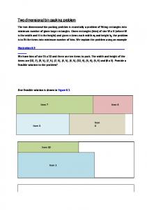
Bin Packing Problem with Conflicts (BPPC). We are given a set V of n items, where each item i has an associated positive weight wi, and n identical bins of ...
Algorithms for the Bin Packing Problem with Conflicts Albert E. Fernandes Muritiba *, Manuel Iori °, Enrico Malaguti*, Paolo Toth* *Dipartimento di Elettronica, Informatica e Sistemistica, Università degli Studi di Bologna, Italy °Dipartimento di Scienze e Metodi dell'Ingegneria, Università degli Studi di Modena e Reggio Emilia, Italy
Outline
Problem Definition LB UB Branch & Price An overall Algorithm Computational Experiments Conclusions
Bin Packing Problem with Conflicts (BPPC)
We are given a set V of n items, where each item i has an associated positive weight wi, and n identical bins of capacity C. In addition, we are given an undirected graph G=(V,E) representing the conflicts between items. The problem is to assign all items to the minimum number of bins without exceeding C and in such a way that no bin contains conflicting items.
1
2
1
3
3
1 C = 6
The BPPC is NPHard: 2 very famous special cases: |E(G)|=0, Bin Packing Problem (BPP) C = ∞, Vertex Coloring Problem (VCP)
Set Covering Formulation for the BPPC
I = family of all the maximal subsets of V representing feasible bins ∈I is used Binary variables: 1 if bin I
xI = {
0 otherwise
min ∑ xI I ∈I
∑x
≥1
∀v ∈ V
(2)
xI ∈ { 0,1}
∀I ∈ I
(3)
I :v∈I
(1)
I
Literature PTAS, special cases, complexity results: H.L. Bodlaender and K. Jansen. On the complexity of scheduling incompatible jobs with unittimes. (1993) P. Hansen, A. Hertz, and J. Kuplinsky. Bounded vertex colorings of graphs. (1993) K. Jansen and S. Oehring. Approximation algorithms for time constrained scheduling. (1997) K. Jansen. An approximation scheme for bin packing with conflicts. (1999) U. Pferschy and J. Schauer. The Knapsack Problem with Conflict Graphs. (2008, available at optimizationonline) Computational paper: M. Gendreau, G. Laporte, and F. Semet. Heuristics and lower bounds for the bin packing problem with conficts. (2004)
Bounding Procedures: BPP Dual feasible functions (Fekete and Schepers 2001) (include the continuous relaxation bound and the bound by Martello and Toth 1990 as special cases)
Bounding Procedures: VCP The cardinality of any clique of the incompatibility graph G represents a LB for the problem. A fast greedy algorithm (Johnson 1974) can be used to compute a maximal clique K of G(V,E): Given an ordering of the vertices, consider the candidate vertices W. Set W=V, K= 0 and iteratively: Choose the vertex v of W of maximum degree and add it to the current clique K. Remove v and all vertices not adjacent to the clique from W.
Gendreau, Laporte and Semet (2004) proposed to consider G’(V,E’) with E’ = E U {(i,j): wi+wj>C} and to compute K’ of G’.
Bounding Procedures: VCP 1
1
2
2
C = 9
2
8 7
E’\E
4
K’
2
2
Problem: “heavy” vertices systematically have a high degree in G’=(V, E’).
E
Bounding Procedures: VCP A different idea: compute a maximal clique K of G=(V,E) through Johnson algorithm. Then, consider G’(V,E’) and expand K to K’’ (possibly different from K’) in G’. On average, |K’’| > |K’|.
1
1
K
2
2
C = 9
2
8 7
4
K’’
E E’\E
2
2
Bounding Procedures: constrained packing lower bound LBcp
Proposed by Gendreau, Laporte and Semet (2004).
Compute a maximal clique K’ of G’ by means of Johnson algorithm;
A bin is used for each of the clique items, and then the largest amount of items that can fit in these bins are inserted, possibly in a fractional way, but by satisfying weight and compatibility constraints. For items which cannot fit, new bins are used;
We propose to improve the maximal clique computation procedure: compute K on graph G and then expand it to K’’ on G’=(V,E’); on average this improves the bound.
Bounding Procedures: Matching 1 5
1 5
C = 10
5
3 bins are needed, but all previous bounds would say that 2 suffice. We propose the following matching based LBmatch: Select (in a greedy fashion) a maximal inclusion subset S of items such that at most 2 can fit into one bin. Let M be a maximum cardinality matching of S on the complement of graph G (compatibility graph).
LBmatch = |M| + ( |S| 2|M| ) = |S| |M| 1 bin for each matched pair 1 bin for “singles”
Greedy Heuristics: GLS Gendreau, Laporte and Semet (2004) propose a set of greedy heuristics:
Some are generalizations of the well known heuristics for the BPP, where items are ordered by non increasing weight and then inserted into bins: First Fit Decreasing, Best Fit Decreasing, Next Fit Decreasing Others integrate procedures for the BPP and VCP in more complex algorithms. We improve these algorithms by considering orderings of the items based on a surrogate weight, which considers also the degree of the items in G:
δ (i ) wi w'i = a + (1 − a ) C |E| with
0 ≤ a ≤1
Evolutionary Algorithm
Inspired from the Evolutionary Algorithm proposed by M., Monaci and Toth for the VCP (2008)
begin Initialize the pool with poolsize solutions while not (problem is solved or timelimit) do Randomly choose two solutions s1, s2 from the pool Apply the crossover to (s1, s2) and generate s3
Improve s3 through the Tabu Search procedure for L iterations
Replace the worst solution in the pool with s3 end
Tabu Search procedure
Solution of the BPPC: partition of the items set V into subsets whose weights do not exceed C and do not contain conflicting items (independent sets).
Impasse Class Neighborhood (VCP, Morgenstern 1996): a target k is required for the number of bins to be used. A solution s is a partition of V in k+1 bins in which all bins except possibly the last one are feasible. Making the bin k+1 empty gives a feasible solution using k bins.
Tabu Search procedure (ctd.) To move from a solution s to a neighbor solution s’: randomly choose an unassigned item v (in bin k+1); assign v to a bin ≤ k, and move all items w of this bin, which are conflicting with v, to bin k+1; continue moving items to bin k+1 until the capacity constraint is not satisfied.
1
2
1
v 1
2
v
1
w 2
w
C = 4
1
2 1
v
2 1
w 2
2
v
1
2
Set Covering Formulation for the BPPC
I = family of all the subsets of V representing feasible bins ∈I is used Binary variables: 1 if bin I
xI = {
0 otherwise
(6)
min z = ∑ xI I ∈I
s.t. (7)
∑x
I :v∈I
I
≥1
xI ∈ { 0,1}
∀v ∈ V
∀I ∈ I
(8)
z *
Solve the LP relaxation of Model (6) – (8), get z*. A valid lower bound is LBSC=
Set Covering Formulation for the BPPC: column generation Model (6) – (8) has an exponential number of variables, thus to solve it we have to use column generation techniques, i.e. to solve a Knapsack Problem with Conflicts (slave problem) to determine the bin of maximum reduced profit:
max ∑ π i zi
(10)
∑w z
(11)
i∈V
i∈V
i i
≤C
zi + z j ≤ 1 zi ∈ { 0,1}
∀i, j : (i, j ) ∈ E i ∈V
(12) (13)
Where πi are the optimal values of the dual variables corresponding to (7)
Set Covering Formulation for the BPPC: column generation In order to solve the Knapsack Problem with Conflicts (slave model (10) – (13)) we use a greedy algorithm: items are considered according to different orderings, and inserted into the knapsack (bin) if they fit. If the greedy algorithm cannot find a positive reduced profit column (bin), we solve model (10) – (13) with Cplex. In order to speed up the computation: • we initialize the set of columns with very good columns from heuristic solutions; • when solving model (10) – (13) with Cplex, we stop as soon as a positive reduced profit column is found; • we replace the incompatibility constraints (12) by a set of stronger clique constraints.
Set Covering Formulation for the BPPC: a Branch&Price algorithm If the solution of the continuous relaxation of model (6) – (8) is not integer, we embed the column generation algorithm in a branching scheme, thus obtaining a Branch&Price algorithm. • We branch on the variables, and choose as branching one the most fractional one (experimentally, faster than branching on the edges) • We first set the branching variables to 1 and then to 0. • We adopt a Depth First strategy.
An overall 4 Phases algorithm We combined in an overall algorithm for BPPC the most effective (according to computational evidence) procedures presented so far. The algorithm starts with fast procedures and, if the problem is not solved, moves to more effective (and time consuming) ones:
I Phase initial LB: DFF and CP improved in the clique computation; initial UB: improved heuristics. If UB=LB stop.
II Phase Evolutionary Algorithm with a given time limit (if the problem is solved for a value of k>LB, we set k=k1 and iterate) . If UB=LB stop.
III Phase solve the continuous relaxation of the set covering formulation SC, thus improving LB (and possibly obtaining the optimal solution if the solution of the SC relaxation is integer). If UB=LB stop
IV Phase – Apply the Branch & Price algorithm.
Computational Experiments
All our programs were written in C and tested on a Pentium IV at 3GHz with 2GB RAM, under Linux operating system.
We compare our results with those obtained by Gendreau, Laporte and Semet (2004). They considered 8 classes of instances from Falkenauer (1996), each class containing 10 BPP instances. By adding, for the instances of each class, random incompatibility graphs with densities varying from 0 to 0.9, they obtained 800 instances (100 for each class).
We generate 800 instances according to their description, and reimplemented their algorithms in order to have a fair (within the limits of our implementation) comparison.
instances are available at www.or.deis.unibo.it
Computational Experiments
When needed, we apply the Evolutionary Algorithm with a time limit of 120 seconds, and we give to the B&P a time limit of 10 hours.
We initialize the pool of columns of the SC formulation with all the columns corresponding to the feasible solutions found by the greedy heuristics and the Evolutionary Algorithm. This speeds up the computation of a factor 2.
Computational Experiments: ratio UB/LB 1,045
1,04 1,035 1,03 1,025
GLS FIMT I Phase
1,02 1,015 1,01 1,005 1
1
2
3
4
5
6
7
8
GLS 222/800 optimal solutions; 2.9 s average computing time FIMT (I Phase) 364/800 optimal solutions; 0.5 s average computing time
Computational Experiments: ratio UB/LB 1,045 1,04 1,035 1,03 1,025
GLS FIMT I Phase FIMT II Phase
1,02 1,015 1,01 1,005 1
1
2
3
4
5
6
7
8
GLS 222/800 optimal solutions; 2.9 s avg. computing time FIMT (I Phase) 364/800 optimal solutions; 0.5 s avg. computing time FIMT (II Phase) 499/800 optimal solutions; 55.0 s avg. computing time
Computational Experiments: ratio UB/LB 1,045 1,04 1,035 1,03 GLS FIMT I Phase FIMT II Phase FIMT III Phase
1,025 1,02 1,015 1,01 1,005 1
1
2
3
4
5
6
7
8
GLS 222/800 optimal solutions; 2.9 s avg. computing time FIMT (I Phase) 364/800 optimal solutions; 0.5 s avg. computing time FIMT (II Phase) 499/800 optimal solutions; 55.0 s avg. computing time FIMT (III Phase) 602/800 optimal solutions; 260.6 s avg. computing time
Computational Experiments: ratio UB/LB 1,007
1,006
1,005
1,004 FIMT III Phase FIMT IV Phase
1,003
1,002
1,001
1
1
2
3
4
5
6
7
8
FIMT (III Phase) 602/800 optimal solutions; 260.6 s avg. computing time FIMT (IV Phase) 780/800 optimal solutions; 1361.1 s avg. computing time (790/800 with a special set up of the parameters)
To conclude
We presented new lower and upper bounds for the BPPC problem, exploiting the double nature of the problem (combination of VCP and BPP).
We proposed an algorithm which integrates fast lower bound computations, heuristics and metaheuristics. Solutions generated during the computation are used to initialize the pool of a Branch & Price algorithm.
Computational experiments show that the new approach improves on previously proposed approaches: in comparable computing time, we can solve 364 (versus 222) instances over 800. With larger computing time, we can solve 780 of 800 instances of the considered set. Thank you for your attention