The two dimensional bin packing problem with side ...

Universität Augsburg Wirtschaftswissenschaftliche Fakultät Lehrstuhl für Health Care Operations/ Health Information Management Prof. Dr. Jens Brunner

The two dimensional bin packing problem with side constraints – Master Thesis –

Academic Advisor:

Prof. Dr. Andreas Fügener

Name:

Markus Seizinger

Filing Date:

11.04.2016

Table of Contents 1.

Introduction .................................................................................................... 1

2.

Literature ........................................................................................................ 4

3.

MIP formulation ............................................................................................ 5

4.

Upper and lower bounds ................................................................................ 8 4.1. Lower bounds ................................................................................................ 8 4.1.1. Geometric bound 𝐿0 ............................................................................... 8 4.1.2. Bound of large items 𝐿1 .......................................................................... 8 4.1.3. Combined bound 𝐿2 .............................................................................. 10 4.1.4. Transforming bound 𝐿3 ........................................................................ 11 4.1.5. One dimensional bin packing problem as lower bound ....................... 12 4.2. Upper bounds ............................................................................................... 19

5.

Solution algorithm ....................................................................................... 22 5.1. Problem decomposition ............................................................................... 22 5.2. Subproblem .................................................................................................. 23 5.3. Subproblem decomposition ......................................................................... 27 5.4. Solution approach ........................................................................................ 28

6.

Numerical Study .......................................................................................... 33 6.1. Instances ....................................................................................................... 33 6.2. Bounds ......................................................................................................... 34 6.3. Algorithm performance ................................................................................ 37

7.

Conclusion ................................................................................................... 41

8.

Publication bibliography .............................................................................. 43

Appendix A ............................................................................................................ 46 Appendix B ............................................................................................................ 48

II

Table of Figures Figure 1: Example packing of 2DBPP-SC .............................................................. 1 Figure 2: Pseudocode of BFDH-SC....................................................................... 20 Figure 3: Packing of BFDH-SC ............................................................................. 21 Figure 4: Pseudocode of 2DPP-SC heuristic ......................................................... 26 Figure 5: Placing items in 2DPP-SC heuristic ....................................................... 26 Figure 6: Column generation algorithm................................................................. 30 Figure 7: Column generation subproblem algorithm ............................................. 31 Figure 8: Distribution of item classes .................................................................... 34

III

List of Tables Table 1: Dimensions of items ................................................................................ 33 Table 2: Summarized lower bounds compared for instance classes ...................... 35 Table 3: Summarized lower bound compared for instance sizes........................... 36 Table 4: Optimally solved instances by 𝐿𝑆𝐶 1𝐷𝐾𝑃 ...................................................... 36 Table 5: Results of column generation algorithm compared by class ................... 38 Table 6: Results of column generation algorithm compared by instance size ....... 39 Table 7: Column generation terminated but not proven optimal ........................... 39 Table 8: Comparison of lower bounds and heuristic per class and instance size .. 48 Table 9: Results of column generation algorithm compared by class and instance size .............................................................................................................................. 49

IV

Abbreviations (1D)BPP

(one dimensional) bin packing problem

1DKP

one dimensional knapsack problem

2DBPP

two dimensional bin packing problem

2DBPP-SC

two dimensional bin packing problem with side constraints

2DPP

two dimensional packing problem

3DBPP

three dimensional bin packing problem

BFDH

best-fit decreasing height

CG

column generation

CT

constraint

iff

if and only if

IP

integer program

LB

lower bound

LP

linear program

MIP

mixed integer program

OPL

Optimization Programming Language

RMP

restricted master problem

UB

upper bound

V

1. Introduction

1. Introduction In the two dimensional bin packing problem with side constraints (2DBPP-SC) we are given a set of rectangular items 𝑖 ∈ 𝐼, each defined by its height ℎ𝑖 , width 𝑤𝑖 and type 𝑡𝑖 . A bin consists of several sides 𝑠 ∈ 𝑆 with dimensions 𝐻 and 𝑊, respectively. The goal of 2DBPP-SC is to assign every item a concrete position such that all items are packed without overlapping and using as few bins as possible. Furthermore, items are packed orthogonally and the newly introduced side constraint has to be fulfilled, meaning that no two items of different type may be placed face-to-face on the same bin but on different sides. We assume items may not be rotated. This problem is an extension of the well-studied two dimensional bin packing problem (2DBPP), where only one bin side exists (|𝑆| = 1). It can as well be reduced to the three dimensional bin packing problem (3DBPP), if only one type of item exists, so |Τ| = 1, and all items 𝑖 ∈ 𝐼 have depth 𝑑𝑖 = 1. 2DBPP-SC is strongly NP-hard, since both 2DBPP and 3DBPP are known to be such (Martello, Vigo 1998; Martello et al. 2000).

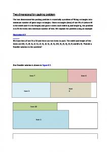
Figure 1: Example packing of 2DBPP-SC

The example depicted in Figure 1 gives an idea of the restrictions implied by the side constraint. This small instance contains bins with two sides (we will speak of front and back side) and two item types. The side constraint reduces the available space on different sides of the bin. In contrast to the traditional 2DBPP, where items simply occupy bin capacity for their respective shape, in 2DBPP-SC items additionally block this capacity on all other sides of the bin. Only items of identical type may use this blocked area (indicated by hatched area). This means that the concrete capacity consumption of a single item depends on the actual packing of the bin. Notice that another item of type A with dimensions (𝑤, ℎ) = (4, 6) could be placed in the bottom 1

1. Introduction right corner on the back side of the bin, whereas an identically shaped item of type B cannot be placed in this position, because it would overlap with area blocked for type A. Bin packing problems are one of the most classical problems known in combinatorial optimization. Nevertheless, the 2DBPP-SC is a new class of problem and has therefore never been formally described nor has any solution algorithm especially designed for this type of problem been published yet. Our interest in this type of problem comes from a real-world application. We analyzed a bottleneck resource in a production process, which was a paint shop. In order to be processed, items had to be placed on racks with two faces (front and rear). Additionally, items were distinguished into two different types. These types were not allowed to be placed face-to-face for quality reasons. Due to these restrictions the utilization of racks was very low and this production step became a limiting factor. 2DBPP-SC corresponds directly to this problem. 2DBPP-SC is an extension of 2DBPP where every bin simply consists of one side. The introduced side-constraint extends the set of cutting patterns, e.g. the well-known guillotine and robot-packable patterns. Lodi et al. (1999) introduced a three field notation to categorize bin packing problems. There, the first position gives the number of dimensions (e.g., BPP, 2DBPP, 3DBPP, …), the second signals whether items may be rotated (R) or are oriented (O), and the third decodes information about any required cutting pattern, like free or guillotine cutting (F, G). Therefore, extending the three field notation of Lodi et al. (1999), 2DBPP-SC can be categorized as 2BP|O|S, meaning that items are oriented (O) and cutting patterns have to apply to the side constraint (S). For the class of 2BP|O|F problems Martello, Vigo (1998) introduced new lower bounds und developed a branch-and-cut algorithm to solve these problems optimally. They furthermore defined new classes of test-instances we will refer to again later. Guillotine-cuttable patterns were recently examined by Lodi et al. (2015), who developed and tested a partial enumeration algorithm for this class of problem. 2DBPP-SC is also related to the bin packing problem with conflicts. Here conflicting items may not be assigned to the same bin, whereas in 2DBPP-SC items of different types may be placed on the same bin but not in certain positions. This problem 2

1. Introduction class got a lot of attention recently by the papers of Muritiba et al. (2010) and Khanafer et al. (2010), who developed new algorithms and lower bounds, as well as Elhedhli et al. (2011) and Sadykov, Vanderbeck (2013), who focused on branch-and-price algorithms. 2DBPP-SC can furthermore be seen as a special case of 3DBPP with bin dimensions 𝐻 × 𝑊 × 𝐷, 𝑑𝑖 = 1, and 𝐷 = |𝑆|, where feasible packings have to apply to the side constraint, additionally. Martello et al. (2000) developed a number of lower bounds derived from lower dimensional cases and described heuristics for filling a single bin, as well as for solving this problem with a branching algorithm especially designed for 3DBPP. The main contribution of this paper is the formal description of the new class of 2DBPP-SC and the application of a column generation (CG) framework. We extend this framework by two different subproblems to speed up the solution process. Those are based on an additional decomposition of the packing problem. Furthermore, we develop a compact MIP formulation for 2DBPP-SC and adapt lower bounds of other bin packing problems, as well as introduce a best-fit heuristic solution algorithm. In an extensive computational study, we present results of the column generation algorithm and compare these to our new lower and upper bounds. A useful set of test instances, derived from literature, is described and introduced. We introduce the compact formulation of 2DBPP-SC in § 3 and show its limitations, which lead to the development of a solution algorithm based on column generation presented in § 5. In § 4 we adapt and improve already known lower bounds from 2DBPP and introduce a new lower bound based on a one dimensional bin packing problem. Also, we apply the well-known best-fit decreasing height (BFDH) heuristic to the side-constraint problem. The performance of the CG algorithm, lower and upper bounds are evaluated for every of four extended instance classes in § 6.

3

2. Literature

2. Literature Regarding the class of 2DBPP much research has already been made focusing on lower bounds, heuristics, and advanced solution algorithms. The survey of Lodi et al. (2002a) provides a great overview over this class and numerous heuristics, based on next-fit, first-fit, and best-fit. Their associated performance ratios are evaluated in Lodi et al. (2002b). Crainic et al. (2008) present another packing-heuristic based on extreme points of already planned items. An exact algorithm using branch-and-bound/cut is presented in Martello, Vigo (1998). Here, items are first sorted according to nonincreasing area. Branching is done at two different levels: the outer branch-decision tree assigns items to bins but does not assign a concrete position. The inner branchdecision tree tries to find a feasible packing for a bin using all currently assigned items. Another exact algorithm based on iteratively dividing items into disjoint groups is presented by Clautiaux et al. (2007). Different initialization methods depending on the structure of items and lower bounds are used to prove optimality. Other solution approaches utilize metaheuristics like tabu search (Lodi et al. 1999) or guided local search (Faroe et al. 2003) and others were investigated by Hopper, Turton (2001). Especially notable is the publication of Pisinger, Sigurd (2007), who were the first to combine column generation (see Lübbecke, Desrosiers (2005) for a great introduction) and constraint programming. The problem is decomposed based on Danzig-Wolfe and split into master and subproblem. The former is a set-covering formulation, whereas the latter is further divided into a one dimensional knapsack problem, responsible for selecting a subset of items, and a constraint-satisfaction problem, which checks whether a feasible packing for those items exists. Column generation is used to solve other 2DBPPs with special cutting pattern requirements, as well (Puchinger, Raidl 2007). Recent publications deal with more specialized cases as done in Dell'Amico et al. (2012), where for a one-dimensional problem precedence relations between items are taken into account and which has great impact on real-world applications in scheduling. In contrast, the problem depicted in Perboli et al. (2012) is based on the generalized bin packing problem and introduces stochastic item profits. This makes the paper especially relevant for fright consolidation scenarios in logistics.

4

3. MIP formulation

3. MIP formulation In this paragraph we formally describe and define a mixed integer problem (MIP) for the 2DBPP-CS. We follow the approach of Pisinger, Sigurd (2007) and define variables forming a coordinate system or grid points, indicating where an item is placed. In contrast to Martello et al. (2007) and Pisinger, Sigurd (2007), who use constraint programming, we rely on a traditional optimization problem. The model assigns every item 𝑖 ∈ 𝐼 a position defined as (𝛼|𝛽|b|s), where 𝛼 ∈ Α and 𝛽 ∈ Β indicate the horizontal and vertical distance of the bottom-left corner of an item to the bottom-left corner of side 𝑠 ∈ 𝑆 of bin 𝑏 ∈ 𝐵, while minimizing the number of bins used. The target function (𝐼) simply counts the number of used bins. Constraints (𝐼𝐼) and (𝐼𝐼𝐼) ensure all items are planned and bins with items in it are counted in (𝐼), respectively. Items must not overlap the edges of a bin (Constraints (𝐼𝑉) ). CTs (𝑉) prevent items from occupying the same coordinates on the same side of a bin, so items do not overlap each other. The side constraint is modeled in (𝑉𝐼) and makes sure only items of the same type occupy the same coordinates on different sides of the same bin. Both sets of variables are defined boolean in CTs (𝑉𝐼𝐼) and (𝑉𝐼𝐼𝐼). The power of this model is limited due to the enormous number of variables and constraints. Even for moderate size instances the model cannot be solved in reasonable time and for larger instances it is even impossible to generate it using ILOG. We therefore introduce a solution algorithm based on decomposition and column generation, which is able to tackle this kind of problem, in § 5. Indices

Sets

𝑖

index for items

∈

𝐼

set of items

𝜏

index for types

∈

Τ

set of types

𝑏

index for bins

∈

𝐵

set of bins

𝑠

index for sides

∈

𝑆

set of sides

𝛼

index for horizontal grid points

∈

Α

set of horizontal grid points

𝛽

index for vertical grid points

∈

Β

set of vertical grid points

5

3. MIP formulation Additional Sets 𝐼 ′ (𝜏) = {𝑖|𝑖 ∈ 𝐼: 𝜏𝑖 = 𝜏} Α = {0,1,2, … , 𝑊 − 1} Β = {0,1,2, … , 𝐻 − 1} Α′ (𝑖, 𝑖 ′ , 𝛼) = {𝛼 ′ |𝛼 ′ ∈ Α: 𝛼 − 𝑤𝑖 ′ < 𝛼 ′ ≤ 𝛼 + 𝑤𝑖 } Β′ (𝑖, 𝑖 ′ , 𝛽) = {𝛽 ′ |𝛽 ′ ∈ Β: 𝛽 − ℎ𝑖 ′ < 𝛽 ′ ≤ 𝛽 + ℎ𝑖 } Parameters 𝑊

width of bin

𝐻

height of bin

𝑀

Large number (Big-M Method; 𝑀 ≥ 𝑊 ∗ 𝐻)

𝑤𝑖

width of item 𝑖

ℎ𝑖

height of item 𝑖

𝜏𝑖

type of item 𝑖

Decision variables 𝑥𝑖𝛼𝛽𝑏𝑠 indicating whether item 𝑖 is placed at (𝛼|𝛽|𝑏|𝑠) 𝑦𝑏

indicating whether bin 𝑏 is used

6

3. MIP formulation

𝑧 2𝐷𝐵𝑃−𝑆𝐶

= min ∑ 𝑦𝑏

(𝐼)

𝑏∈𝐵

∑ ∑ ∑ ∑ 𝑥𝑖𝛼𝛽𝑏𝑠

𝑠. 𝑡.:

=

1

∀𝑖 ∈𝐼

(II)

𝑥𝑖𝛼𝛽𝑏𝑠 − 𝑦𝑏

≤

0

∀ 𝑖 ∈ 𝐼, 𝛼 ∈ Α, 𝛽 ∈ Β, 𝑏 ∈ 𝐵, 𝑠 ∈ 𝑆

(III)

𝑥𝑖𝛼𝛽𝑏𝑠

=

0

∀ 𝑖 ∈ 𝐼, 𝛼 ∈ Α, 𝛽 ∈ Β, 𝑏 ∈ 𝐵, 𝑠 ∈ 𝑆:

(𝐼𝑉)

𝛼∈Α 𝛽∈Β 𝑏∈𝐵 𝑠∈𝑆

𝛼 + 𝑤𝑖 > 𝑊 ∨ 𝛽 + ℎ𝑖 > 𝐻 𝑀(𝑥𝑖𝛼𝛽𝑏𝑠 − 1) + ∑

∑

∑

𝑥𝑖 ′ 𝛼′ 𝛽′ 𝑏𝑠

≤

1

∀ 𝑖 ∈ 𝐼, 𝛼 ∈ Α, 𝛽 ∈ Β, 𝑏 ∈ 𝐵, 𝑠 ∈ 𝑆

(𝑉)

∑ 𝑥𝑖 ′ 𝛼′ 𝛽′ 𝑏𝑠′

≤

0

∀ 𝑖 ∈ 𝐼, 𝛼 ∈ Α, 𝛽 ∈ Β, 𝑏 ∈ 𝐵, 𝑠 ∈ 𝑆

(𝑉𝐼)

𝑏𝑖𝑛𝑎𝑟𝑦 ∀ 𝑖 ∈ 𝐼, 𝛼 ∈ Α, 𝛽 ∈ Β, 𝑏 ∈ 𝐵, 𝑠 ∈ 𝑆

(𝑉𝐼𝐼)

𝑏𝑖𝑛𝑎𝑟𝑦 ∀ 𝑡 ∈ 𝑇

(𝑉𝐼𝐼𝐼)

𝑖 ′ ∈𝐼 𝛼′ ∈Α′ (𝑖,𝑖 ′ ,𝛼) 𝛽 ′ ∈Β′ (𝑖,𝑖 ′ ,𝛽)

𝑀(𝑥𝑖𝛼𝛽𝑏𝑠 − 1) +

∑

∑

∑

𝑖 ′ ∈𝐼\𝐼 ′ (𝜏𝑖 ) 𝛼′ ∈Α′ (𝑖,𝑖 ′ ,𝛼) 𝛽 ′ ∈Β′ (𝑖,𝑖 ′ ,𝛽) 𝑠′ ∈𝑆\{𝑠}

𝑥𝑖𝛼𝛽𝑏𝑠 𝑦𝑡

7

4. Upper and lower bounds

4. Upper and lower bounds When trying to find a solution to an optimization problem tight upper and lower bounds are crucial and can speed up the solution process dramatically. In a minimization problem any feasible solution is a primal or upper bound, whereas any relaxation will act as a dual or lower bound. In this chapter we will introduce several lower bounds as well as a best-fit algorithm generating feasible solutions.

4.1. Lower bounds We introduce already known lower bounds for 2DBPP and 3DBPP and adapt them to our new class of 2DBPP-SC. We furthermore present a new lower bound based on a 1DBPP formulation, and prove that it dominates all other known bounds. 4.1.1. Geometric bound 𝑳𝟎 The geometric or continuous lower bound 𝐿0 is obtained by allowing items to be divided into multiple smaller geometric shapes and has already been applied to 2DBPP in several publications (Berkey, Wang 1987; Martello, Vigo 1998; Lodi et al. 2002a). Martello, Vigo (1998) give prove that the asymptotic worst case performance ratio is 1

. By neglecting item types and adapting the concept of a bin consisting of multiple

4

sides, this bound can easily be reformulated for 2DBPP-SC, as well. The bound is calculated by summing up the area of all items, dividing it by the area available in one bin, and rounding it up to the next integer. ∑𝑖∈𝐼 𝑤𝑖 ∗ ℎ𝑖 𝐿𝑆𝐶 ⌉ 0 =⌈ 𝑊 ∗ 𝐻 ∗ |𝑆| This bound can be calculated in linear time with respect to the number of items. 4.1.2. Bound of large items 𝑳𝟏 𝐿0 was the only known lower bound for 2DBPP until the work of Martello, Vigo (1998) and as well for 3DBPP until Martello et al. (2000), who introduced new bounds derived from one-dimensional problems. We adapt the bound of large items 𝐿3𝐷𝐵𝑃 (Martello et al. 2000), which was 1 originally designed for 3DBPP, to obtain a new lower bound for 2DBPP-SC. In the three dimensional case items are assigned to multiple sets 𝐼𝑙 (𝑝), 𝐼𝑠 (𝑝) ⊆ 𝐼𝑙𝑎𝑟𝑔𝑒 ⊆ 𝐼 according to their dimensions. Note that items in 𝐼𝑙𝑎𝑟𝑔𝑒 are strictly larger than half of 8

4. Upper and lower bounds the bin in width and height and can therefore only be packed into the same bin by placing them one behind another. Additionally, the set 𝐼𝑙 (𝑝) contains items, which are deeper than half of the bin. 𝐼𝑠 (𝑝) consist of items 𝑖 ∈ 𝐼𝑙𝑎𝑟𝑔𝑒 \ 𝐼𝑙 (𝑝) at least as deep as 𝑝. The bound is made up from two different terms. The first one simply counts the number of elements that cannot be placed in the same bin. The second term evaluates how many additional bins are required for packing the remaining items by taking their depth into account. 𝐼𝑙𝑎𝑟𝑔𝑒 = {𝑖|𝑖 ∈ 𝐼: 𝑤𝑖 >

𝑊 𝐻 ∧ ℎ𝑖 > } 2 2

𝐼𝑙 (𝑝) = {𝑖|𝑖 ∈ 𝐼𝑙𝑎𝑟𝑔𝑒 : |𝑆| − 𝑝 ≥ 𝑑𝑖 >

𝐼𝑠 (𝑝) = {𝑖|𝑖 ∈ 𝐼𝑙𝑎𝑟𝑔𝑒 :

𝐿3𝐷𝐵𝑃 = |{𝑖|𝑖 ∈ 𝐼𝑙𝑎𝑟𝑔𝑒 : 𝑑𝑖 > 1

|𝑆| } 2

|𝑆| ≥ 𝑑𝑖 ≥ 𝑝} 2

∑𝑖∈𝐼𝑠 (𝑝) 𝑑𝑖 − (|𝐼𝑙 (𝑝)||𝑆| − ∑𝑖∈𝐼𝑙(𝑝) 𝑑𝑖 ) |𝑆| }| + max { } |𝑆| |𝑆| 2 1≤𝑝≤ 2

For 2DBPP-SC this bound simplifies quite a lot. Since in 2DBPP-SC it holds for all items 𝑖 ∈ 𝐼 that 𝑑𝑖 = 1, the cardinality of the set {𝑖|𝑖 ∈ 𝐼𝑙𝑎𝑟𝑔𝑒 : 𝑑𝑖 > zero, because no item applies to the stated condition 𝑑𝑖 >

|𝑆| 2

|𝑆| 2

} is equal to

. Remember that in

2DBPP-SC, |𝑆| is defined to be strictly larger than one, since otherwise the problem would degenerate to 2DBPP. For the same reason, for any 𝑝 it holds that 𝐼𝑙 (𝑝) = ∅. On the other hand, it is easy to see that 𝐼𝑠 (1) = 𝐼𝑙𝑎𝑟𝑔𝑒 and 𝐼𝑠 (𝑝) = ∅ for any other 𝑝. So, the bound consists only of counting those items, which cannot be placed on the same side of a bin, and can be strengthened by taking item types into account. No two items of 𝐼𝑠 (1) that are of different type can be placed in the same bin. We therefore extend this set to 𝐼𝑠 (𝑝, 𝜏) = 𝐼𝑠 (𝑝) ∩ 𝐼′(𝜏), which devides 𝐼𝑠 (𝑝) into disjoint subsets containing only items of a certain type 𝜏. This leads to the following formulation: 𝐿𝑆𝐶 1 =∑ 𝜏∈Τ

|𝐼𝑠 (1, 𝜏)| |𝑆|

The worst case performance of this bound is arbitrarily bad. This can be easily seen at an instance, where no item is strictly larger and wider than half of the bin’s 9

4. Upper and lower bounds dimensions, so 𝐼𝑙𝑎𝑟𝑔𝑒 = ∅ and 𝐿𝑆𝐶 1 = 0. The bound can as well be calculated in linear time with respect to the number of items (Martello et al. 2000). 4.1.3. Combined bound 𝑳𝟐 The second newly introduced bound is a combination of geometry and large items and we therefore call it the combined bound 𝐿𝑆𝐶 2 . This bound was introduced by Martello et al. (2000) and is originally designed for 3DBPP, too. Again, items are assigned to different disjoint subsets, with respect to parameters 𝑝, 𝑞. Note that for 𝑝 = 1, 𝑞 = 1 all items are taken into account, so 𝐼1 (1,1) ∪ 𝐼2 (1,1) ∪ 𝐼3 (1,1) = 𝐼. For all other 𝑝, 𝑞 only a strict subset of items 𝐼1 (1,1) ∪ 𝐼2 (1,1) ∪ 𝐼3 (1,1) ⊂ 𝐼 is considered. Also notice that 𝐼1 (𝑝, 𝑞) ∪ 𝐼2 (𝑝, 𝑞) = 𝐼𝑙𝑎𝑟𝑔𝑒 from 𝐿1 . 𝐿2 strengthens the value of 𝐿1 by adding an additional term. This second term calculates a lower bound on the number of bins needed for items in 𝐼3 (𝑝, 𝑞) geometrically. In bins (sides) with an item of 𝐼1 (𝑝, 𝑞) no other item can fit. Therefore, these very large items 𝑖 ∈ 𝐼1 (𝑝, 𝑞) are considered with dimensions 𝑊 × 𝐻 × 𝑑𝑖 . In bins (sides) that contain an item of 𝐼2 other items of 𝐼3 may fit. Their concrete shape is neglected but their area is summed up and the area available in 𝐼2 -bins is subtracted from that value. This latter value is again divided by the bin area and rounded to the next integer. The three dimensional bound can be calculated as follows: 𝐼1 (𝑝, 𝑞) = {𝑖 ∈ 𝐼: 𝑤𝑖 > 𝑊 − 𝑝 ∧ ℎ𝑖 > 𝐻 − 𝑞} 𝐼2 (𝑝, 𝑞) = {𝑖 ∈ 𝐼 \ 𝐼1 (𝑝, 𝑞): 𝑤𝑖 >

𝑊 𝐻 ∧ ℎ𝑖 > } 2 2

𝐼3 (𝑝, 𝑞) = {𝑖 ∈ 𝐼 \ ( 𝐼1 (𝑝, 𝑞) ∪ 𝐼2 (𝑝, 𝑞) ): 𝑤𝑖 ≥ 𝑝 ∧ ℎ𝑖 ≥ 𝑞} 𝐿3𝐷𝐵𝑃 2 =

𝐿3𝐷𝐵𝑃 1

∑𝑖∈𝐼2 (𝑝,𝑞)∪𝐼3 (𝑝,𝑞) 𝑤𝑖 ℎ𝑖 𝑑𝑖 − (|𝑆|𝐿3𝐷𝐵𝑃 − ∑𝑖∈𝐼1 (𝑝,𝑞) 𝑑𝑖 )𝑊𝐻 1 + max {0, ⌈ ⌉} 𝑊 𝐻 𝑊 ∗ 𝐻 ∗ |𝑆| 1≤𝑝≤ ; 1≤𝑞≤ 2

2

Since in 2DBPP-SC depth is defined to be 𝑑𝑖 = 1 for all items 𝑖 ∈ 𝐼 the analogous bound 𝐿𝑆𝐶 2 can be simplified. Again, item types cannot be respected in the geometric part of this bound. Thus, the combined bound for 2DBPP-SC is 𝐿𝑆𝐶 2

=

𝐿𝑆𝐶 1

∑𝑖∈𝐼2 (𝑝,𝑞)∪𝐼3 (𝑝,𝑞) 𝑤𝑖 ℎ𝑖 − (|𝑆|𝐿𝑆𝐶 1 − |𝐼1 (𝑝, 𝑞)|)𝑊𝐻 + max {0, ⌈ ⌉} 𝑊 𝐻 𝑊𝐻|𝑆| 1≤𝑝≤ ; 1≤𝑞≤ 2

2

10

4. Upper and lower bounds It is obvious that both 𝐿2 -bounds dominate their respective 𝐿1 . Furthermore, for (𝑝, 𝑞) = (1,1) both bounds dominate 𝐿0 since all items are considered at least geometrically. Items in 𝐼1 are “virtually enlarged” to dimensions 𝑊 × 𝐻 × 𝑑𝑖 , items in 𝐼2 and 𝐼3 are assumed with their original dimensions. For a more formal proof see proposition 3 in Martello et al. (2000). This bound can be computed in polynomial time with respect to number of items and bin dimensions. 4.1.4. Transforming bound 𝑳𝟑 The third bound, called transforming bound L3 , is adapted from a two-dimensional bound by Martello, Vigo (1998) which is again based on large items and a relaxed consideration of smaller items and might “in some cases improve” (Martello, Vigo 1998) the combined bound. The number of bins needed for large items is again strengthened by adding the lower bound on “bins needed for those pieces of 𝐼3 that cannot be packed into the bins used for pieces of 𝐼2 ” (Martello, Vigo 1998) but in contrast to 𝐿2 the actual shape of items in 𝐼3 is respected. The latter value is calculated based on a relaxation. 𝑚(𝑖, 𝑝, 𝑞) gives the maximum number of items in 𝐼3 with dimensions 𝑤𝑖 = 𝑝, ℎ𝑖 = 𝑞 that can be packed into (a side of) a bin, which already contains item 𝑖 ∈ 𝐼2 , by packing them above and/or besides of 𝑖. Here, the dimensions of items larger than 𝑝 × 𝑞 are relaxed and assumed to be 𝑝 × 𝑞. These items are said to be transformed. The original two dimensional bound is computed like this: 𝑊 𝐻 − ℎ𝑖 𝐻 𝑊 − 𝑤𝑖 𝑊 − 𝑤𝑖 𝐻 − ℎ𝑖 𝑚(𝑖, 𝑝, 𝑞) = ⌊ ⌋ ⌊ ⌋ + ⌊ ⌋⌊ ⌋−⌊ ⌋⌊ ⌋ 𝑝 𝑞 𝑞 𝑝 𝑝 𝑞

𝐿2𝐷𝐵𝑃 = |𝐼𝑙𝑎𝑟𝑔𝑒 | + 3

|𝐼3 (𝑝, 𝑞)| − ∑𝑖∈𝐼2 (𝑝,𝑞) 𝑚(𝑖, 𝑝, 𝑞) {0; ⌈ ⌉} 𝑊 𝐻 𝑊 𝐻 1≤𝑝≤ ; 1≤𝑞≤ ⌊ 𝑝 ⌋ ⌊𝑞 ⌋ 2 2 max

The bound is applied to 2DBPP-SC by altering both addends. The cardinality of large items is equivalent to the previously introduced bound 𝐿𝑆𝐶 1 in 2DBPP-SC. The second term – the number of bins needed for pieces that do not fit into bins already created for larger items – must take multiple item sides into account. The denominator is therefore multiplied by the number of bin sides |𝑆|.

𝑆𝐶 𝐿𝑆𝐶 3 = 𝐿1 +

max

𝑊 𝐻 1≤𝑝≤ ; 1≤𝑞≤ 2 2

{0;

|𝐼3 (𝑝, 𝑞)| − ∑𝑖∈𝐼2 (𝑝,𝑞) 𝑚(𝑖, 𝑝, 𝑞) } 𝑊 𝐻 ⌊ 𝑝 ⌋ ⌊ 𝑞 ⌋ ∗ |𝑆| 11

4. Upper and lower bounds Obviously, both 𝐿3 bounds dominate their respective 𝐿1 counterparts. However, no dominance relation between 𝐿2 and 𝐿3 exists. This can be easily shown by two small example

instances:

Imagine

an

instance

with

bin

dimensions

𝑊 × 𝐻 × 𝐷 = 10 × 10 × 2 and items with 𝑤1 = ℎ1 = 8 and 𝑤𝑖 = ℎ𝑖 = 3 for 𝑆𝐶 𝑖 = 2, … , 5, all of same type. The bounds take the values 𝐿0 = 𝐿𝑆𝐶 1 = 𝐿2 = 1 and

𝐿𝑆𝐶 3 = 2. For another instance with 9 items with 𝑤1 = ℎ1 = 3 and 𝑤𝑖 = ℎ𝑖 = 5 for 𝑆𝐶 𝑖 = 2, … , 9 the bounds are 𝐿0 = 𝐿𝑆𝐶 2 = 2, 𝐿1 = 0 and 𝐿3 = 1. For a corresponding

proof on dominance between 𝐿2𝐷𝐵𝑃 and 𝐿2𝐷𝐵𝑃 we refer to Martello, Vigo (1998). 2 3 4.1.5. One dimensional bin packing problem as lower bound We present a new lower bound for 2DBPP-SC in form of an IP model based on a one dimensional bin packing formulation. We furthermore prove that this new bound dominates all previously introduced bounds. In this model we determine a lower bound on the optimal value of 2DBPP-SC by reducing both bins and items to one-dimensional objects. Notice that bins still consist of multiple sides, so the capacity of a side is 𝑊 × 𝐻 and of a bin is 𝑊 × 𝐻 × |𝑆|. Correspondingly, the weight or utilization of an item 𝑖 is 𝑤𝑖 × ℎ𝑖 . We adapt the ideas of previously introduced bounds and transfer them to (M)IP models. Items are assigned to bins with respect to capacity restrictions for every side of this bin (this corresponds to 𝐿0 ). Additionally, an advanced capacity constraint, based on item types on different sides of the same bin, is applied. Finally, we investigate every individual pair of items and determine whether this pair can be packed in the same side or in the same bin in a 2DBPP-SC scenario. We therefore transfer the idea of the bound of large items 𝐿𝑆𝐶 1 .

12

4. Upper and lower bounds Indices

Sets

𝑖

index for items

∈

𝐼

set of items

𝜏

index for types

∈

Τ

set of types

𝑏

index for bins

∈

𝐵

set of bins

𝑠

index for sides

∈

𝑆

set of sides

Additional Sets 𝐼𝜏 = {𝑖|𝑖 ∈ 𝐼: 𝜏𝑖 = 𝜏} 𝐼̃𝑖 = {𝑖 ′ |𝑖 ′ ∈ 𝐼 ∶ ℎ𝑖 + ℎ𝑖 ′ > 𝐻 ∧ 𝑤𝑖 + 𝑤𝑖 ′ > 𝑊 ∧ 𝑖 ≠ 𝑖 ′ } 𝐼̅𝑖 = {𝑖′ |𝑖′ ∈ 𝐼̃𝑖 ∶ 𝜏𝑖 ≠ 𝜏𝑖′ } Parameters 𝑊

width of bin

𝐻

height of bin

𝑤𝑖

width of item 𝑖

ℎ𝑖

height of item 𝑖

𝜏𝑖

type of item 𝑖

Decision variables 𝑥𝑖𝑏𝑠

indicating whether item 𝑖 is placed on side 𝑠 of bin 𝑏

𝑦𝑏

indicating whether bin 𝑏 is used

Expressions ̅ 𝜏𝑏𝑠 = ∑ 𝑤𝑖 ∗ ℎ𝑖 ∗ 𝑥𝑖𝑏𝑠 𝐴

volume occupied by items of type 𝜏 on side 𝑠 of bin 𝑏

𝑖∈𝐼𝜏

13

4. Upper and lower bounds min ∑ 𝑦𝑏 𝐿𝑆𝐶 1𝐷𝐵𝑃 =

(I)

𝑏∈𝐵

𝑠. 𝑡.:

∑ ∑ 𝑥𝑖𝑏𝑠

= 1

∀𝑖 ∈𝐼

(II)

∀ 𝑖 ∈ 𝐼, 𝑏 ∈ 𝐵, 𝑠 ∈ 𝑆

(III)

∀ 𝑏 ∈ 𝐵, 𝑠 ∈ 𝑆

(IV)

∀𝑏 ∈ 𝐵, 𝑠, 𝑠′ ∈ 𝑆, 𝜏 ∈ T

(V)

𝑥𝑖𝑏𝑠 + 𝑥𝑖′ 𝑏𝑠 ≤ 1

∀ 𝑖 ∈ 𝐼, 𝑖 ′ ∈ 𝐼̃𝑖 , 𝑏 ∈ 𝐵, 𝑠 ∈ 𝑆

(VI)

𝑥𝑖𝑏𝑠 + 𝑥𝑖′ 𝑏𝑠′ ≤ 1

∀ 𝑖 ∈ 𝐼, 𝑖 ′ ∈ 𝐼𝑖̅ , 𝑏 ∈ 𝐵, 𝑠, 𝑠′ ∈ 𝑆

(VII)

∀𝑖 ∈ 𝐼, 𝑏 ∈ 𝐵, 𝑠 ∈ 𝑆

(VIII)

𝑏∈𝐵 𝑠∈𝑆

𝑥𝑖𝑏𝑠 − 𝑦𝑏 ≤ 0 ∑ 𝑤𝑐 ∗ ℎ𝑐 ∗ 𝑥𝑖𝑏𝑠

≤ 𝑊∗𝐻

𝑖∈𝐼

̅ 𝜏𝑏𝑠 + ∑ 𝐴 ̅ ′ ′ 𝐴 𝜏 𝑏𝑠 ≤ 𝑊∗𝐻 𝜏′ ∈Τ\{𝜏}

𝑥𝑖𝑏𝑠 𝑏𝑜𝑜𝑙𝑒𝑎𝑛 𝑦𝑏 𝑏𝑜𝑜𝑙𝑒𝑎𝑛

∀𝑏 ∈𝐵

(IX)

The target function (𝐼) counts the number of used traverses. Constraints (𝐼𝐼) (in combination with (𝑉𝐼𝐼𝐼)) force every item to be assigned to exactly one bin. Constraints (𝐼𝐼𝐼) activate bins with at least one item assigned to them. Capacity restriction is modeled in CTs (𝐼𝑉), making sure that the volume of assigned items does not exceed the volume of a bin’s side. CTs (𝑉) are advanced capacity constraints; The ̅ 𝜏𝑡𝑠 . By the properties volume of items of a type 𝜏 on side 𝑠 of bin 𝑏 are summed up to 𝐴

of 2DBPP-SC we know that volume occupied by other types 𝜏′ on other sides 𝑠′ is blocked and this causes the reduction of available volume on this side to 𝑊 ∗ 𝐻 − ∑𝜏′ ∈Τ\{𝜏} 𝐴̅𝜏′ 𝑏𝑠′ . Similar to the idea of 𝐿𝑆𝐶 1 , we investigate every individual pair of items 𝑖, 𝑖 ′ and check if they can be packed in the same side (CTs (𝑉𝐼)) or in the same bin (CTs (𝑉𝐼𝐼)) from a two-dimensional point of view. These checks are performed based on item dimensions. If 𝑤𝑖 + 𝑤𝑖 ′ > 𝑊 (ℎ𝑖 + ℎ𝑖 ′ > 𝐻), both items cannot be placed side by side (one on top of the other). For items 𝑖 ′ ∈ 𝐼̃𝑖 , we can say they are in conflict to item 𝑖 and forbid them to be placed on the same side of a bin. Notice that two such items may, though, be placed in the same bin. Similarly, if both items additionally are of different types, so 𝑖 ′ ∈ 𝐼𝑖̅ , items may even not be assigned to the same bin. Finally, constraints (𝑉𝐼𝐼𝐼) and (𝐼𝑋) define both sets of decision variables to be boolean. The model above is a relaxation of 2DBPP-SC, hence 𝐿𝑆𝐶 1𝐷𝐵𝑃 is a valid lower bound on 𝑧 2𝐷𝐵𝑃−𝑆𝐶 . Constraints (𝐼𝐼) and (𝐼𝐼𝐼) are identical in both models, besides the fact 14

4. Upper and lower bounds that an item is not assigned a concrete position but solely to a side of a bin. The block of constraints (𝐼𝑉) to (𝑉𝐼) in the 2D model, making sure items do not overlap the bin or each other, are reformulated to capacity restrictions (𝐼𝑉), (𝑉) and conflict CTs (𝑉𝐼) and (𝑉𝐼𝐼) in the 1D case. As already mentioned, a one dimensional bin packing problem is NP-hard in the strong sense, hence 1DBPP-SC is as well. Nevertheless, this problem can be solved quite efficiently by providing the solver a lower bound to the solution value by using one or more of the previously introduced bounds. Additionally, by applying a heuristic (see next sub-paragraph) one can obtain a good primal bound and bring it to the problem by setting |𝐵 | = 𝑈𝐵. These steps can drastically reduce the effort for solving this problem. Notice that the emphasis of the solution process should be to improve the dual bound, because this is the only improvement of interest. In the following, we prove that 𝐿𝑆𝐶 1𝐷𝑃𝐵 dominates all other bounds by converting every bound to an IP or MIP formulation and show that every of these models is a relaxation of 𝐿𝑆𝐶 1𝐷𝑃𝐵 . We will, from now on for the rest of this paragraph, refer to the constraints of 𝐿𝑆𝐶 1𝐷𝑃𝐵 with (𝐼) to (𝐼𝑋). In the following models we will mark relaxations of those CTs by an apostrophe, (𝐼 ′ ) to (𝐼𝑋 ′ ). Dominance over 𝑳𝟎 The geometric or continuous lower bound 𝐿0 allows items to be cut into smaller pieces, so it only takes volumes into account and does not make any use of item types. Hence, this bound can be modeled as follows. 𝑧 𝐿0

=

min ∑ 𝑦𝑏

(I)

𝑏∈𝐵

∑ ∑ 𝑥𝑖𝑏𝑠 =

𝑠. 𝑡.:

1

∀𝑖 ∈𝐼

(II)

𝑏∈𝐵 𝑠∈𝑆

𝑥𝑖𝑏𝑠 − 𝑦𝑏

≤

0

∀ 𝑖 ∈ 𝐼, 𝑏 ∈ 𝐵, 𝑠 ∈ 𝑆

(III)

∑ 𝑤𝑖 ∗ ℎ𝑖 ∗ 𝑥𝑖𝑏𝑠

≤

𝑊∗𝐻

∀𝑏 ∈ 𝐵, 𝑠 ∈ 𝑆

(IV)

≥

0

∀𝑖 ∈ 𝐼, 𝑏 ∈ 𝐵, 𝑠 ∈ 𝑆

𝑖∈𝐼

𝑥𝑖𝑏𝑠

𝑦𝑏 𝑏𝑜𝑜𝑙𝑒𝑎𝑛

∀𝑏 ∈𝐵

(VIII‘) (IX)

15

4. Upper and lower bounds In this model constraints (𝐼𝐼) to (𝐼𝑉) match the original constraints. Every item has to be planned (completely), bins with items assigned to it must be marked as used, and capacity restrictions of bin sides are still valid, as well. The original constraints (𝑉) to (𝑉𝐼𝐼) were dropped, because this bound does not distinguish between item types and cannot consider conflicts. Constraints (𝑉𝐼𝐼𝐼 ′ ) relaxe the integrity condition of variable 𝑥, so items may be split into multiple parts and may be placed in several bins. Hence, this model is equivalent to bound 𝐿0 and is a relaxation of 𝐿𝑆𝐶 1𝐷𝐵𝑃 . Dominance over 𝑳𝑺𝑪 𝟏 𝑙𝑎𝑟𝑔𝑒 In contrast to 𝐿0 , the bound of large items 𝐿𝑆𝐶 1 considers conflicting items in 𝐼

and their associated item types but does not utilize any geometry and neglects all remaining items 𝐼\𝐼𝑙𝑎𝑟𝑔𝑒 . It counts the number of bins needed for these large items respecting conflicts. This bound can be modeled as: 𝑆𝐶

𝑧 𝐿1

= min ∑ 𝑦𝑏

(I)

𝑏∈𝐵

𝑠. 𝑡.:

∑ ∑ 𝑥𝑖𝑏𝑠 = 1

∀ 𝑖 ∈ 𝐼𝑙𝑎𝑟𝑔𝑒

(II‘)

∀ 𝑖 ∈ 𝐼𝑙𝑎𝑟𝑔𝑒 , 𝑏 ∈ 𝐵, 𝑠 ∈ 𝑆

(III‘)

∀ 𝑖, 𝑖 ′ ∈ 𝐼𝑙𝑎𝑟𝑔𝑒 , 𝑏 ∈ 𝐵, 𝑠 ∈ 𝑆: 𝑖 ≠ 𝑖 ′

(VI‘)

∀ 𝑖, 𝑖 ′ ∈ 𝐼𝑙𝑎𝑟𝑔𝑒 , 𝑏 ∈ 𝐵, 𝑠, 𝑠 ′ ∈ 𝑆:

(VII‘)

𝑏∈𝐵 𝑠∈𝑆

𝑥𝑖𝑏𝑠 − 𝑦𝑏 ≤ 0 𝑥𝑖𝑏𝑠 + 𝑥𝑖 ′ 𝑏𝑠 ≤ 1 𝑥𝑖𝑏𝑠 + 𝑥𝑖 ′ 𝑏𝑠′ ≤ 1

𝑡𝑖 ≠ 𝑡𝑖 ′ 𝑥𝑖𝑏𝑠 𝑏𝑜𝑜𝑙𝑒𝑎𝑛 𝑦𝑏 𝑏𝑜𝑜𝑙𝑒𝑎𝑛

∀𝑖 ∈ 𝐼𝑙𝑎𝑟𝑔𝑒 , 𝑏 ∈ 𝐵, 𝑠 ∈ 𝑆 ∀𝑏 ∈𝐵

(VIII‘) (IX)

The set of items 𝐼 is relaxed to only large items 𝐼𝑙𝑎𝑟𝑔𝑒 in CTs (𝐼𝐼 ′ ) to (𝑉𝐼𝐼𝐼 ′ ), because all other items are ignored. Besides this, these constraints are basically identical to their respective originals. Furthermore, constraints (𝐼𝑉) and (𝑉), which model bin capacity, are dropped, because the bound does not reflect geometry of any item. Again it is easy to see this model is a relaxation of 𝐿𝑆𝐶 1𝐷𝐵𝑃 . Dominance over 𝑳𝑺𝑪 𝟐 𝑆𝐶

𝑆𝐶 𝐿1 The combined bound 𝐿𝑆𝐶 a lower bound on the 2 adds to the value of 𝐿1 or 𝑧

number of bins for items of 𝐼3 (𝑝, 𝑞), derived from geometry of those items. So, the 16

4. Upper and lower bounds MIP formulation of this bound is a combination of the previous models, as well. 𝑆𝐶

Parallel to 𝑧 𝐿1 , all constraints for 𝐼 (𝐶𝑇𝑠 (𝐼𝐼′) to (𝑉𝐼𝐼′)) are relaxed to 𝐼 ′ (𝑝, 𝑞), which is a less strict relaxation than 𝐼𝑙𝑎𝑟𝑔𝑒 , so 𝐼𝑙𝑎𝑟𝑔𝑒 ⊆ 𝐼 ′ (𝑝, 𝑞), for any (𝑝, 𝑞) as already proved. To account for the additional maximization term in 𝐿𝑆𝐶 2 , the domain of decision variables 𝑥𝑖𝑏𝑠 is relaxed for all 𝑖 ∈ 𝐼3 (𝑝, 𝑞) in constraints (𝑉𝐼𝐼𝐼 𝑏 ′ ). The bound requires the remaining items to be placed in one bin as a whole. The corresponding variables are defined as boolean for these 𝑖 ∈ 𝐼 ′ (𝑝, 𝑞)\𝐼3 (𝑝, 𝑞). Constraints (𝑉𝐼 ′ ) and (𝑉𝐼𝐼 ′ ) ensure that conflicts between items in 𝐼1 and 𝐼2 and between items in 𝐼1 and 𝐼3 are respected. The original constraint (𝑉) is dropped, because item types are ignored by this bound in extend to CTs (𝑉𝐼𝐼 ′ ). (I)

𝑆𝐶 𝑧 𝐿2 (𝑝, 𝑞) = min ∑ 𝑦𝑏

𝑏∈𝐵

𝑠. 𝑡.:

∑ ∑ 𝑥𝑖𝑏𝑠 = 1

(II‘)

∀ 𝑖 ∈ 𝐼 ′ (𝑝, 𝑞)

𝑏∈𝐵 𝑠∈𝑆

𝑥𝑖𝑏𝑠 − 𝑦𝑏 ≤ 0 ∑ 𝑤𝑖 ℎ𝑖 𝑥𝑖𝑏𝑠 ≤ 𝑊 𝐻

∀ 𝑖 ∈ 𝐼 ′ (𝑝, 𝑞), 𝑏 ∈ 𝐵, 𝑠 ∈ 𝑆

(III‘) (IV‘)

∀ 𝑏 ∈ 𝐵, 𝑠 ∈ 𝑆

𝑖∈𝐼 ′ (𝑝,𝑞)

𝑥𝑖𝑏𝑠 + 𝑥𝑖 ′ 𝑏𝑠 ≤ 1

∀ 𝑖 ∈ 𝐼1 (𝑝, 𝑞), 𝑖 ′ ∈ 𝐼 ′ (𝑝, 𝑞)\{𝑖},

(VI‘)

𝑏 ∈ 𝐵, 𝑠 ∈ 𝑆 𝑥𝑖𝑏𝑠 + 𝑥𝑖 ′ 𝑏𝑠′ ≤ 1

∀ 𝑖 ∈ 𝐼1 (𝑝, 𝑞), 𝑖 ′ ∈ 𝐼 ′ (𝑝, 𝑞)\{𝑖},

(VII‘)

𝑏 ∈ 𝐵, 𝑠, 𝑠 ′ ∈ 𝑆: 𝜏𝑖 ≠ 𝜏𝑖 ′ 𝑥𝑖𝑏𝑠 𝑏𝑜𝑜𝑙𝑒𝑎𝑛

∀𝑖 ∈ 𝐼1 (𝑝, 𝑞) ∪ 𝐼2 (𝑝, 𝑞),

(VIII a‘)

𝑏 ∈ 𝐵, 𝑠 ∈ 𝑆 𝑥𝑖𝑏𝑠 ≥ 0 𝑦𝑏 𝑏𝑜𝑜𝑙𝑒𝑎𝑛

∀𝑖 ∈ 𝐼3 (𝑝, 𝑞), 𝑏 ∈ 𝐵, 𝑠 ∈ 𝑆

(VIII b‘)

∀𝑏 ∈𝐵

(IX)

𝑆𝐶

𝑆𝐶 Notice that for every (𝑝, 𝑞) it holds that 𝑧 𝐿2 (𝑝, 𝑞) ≤ 𝑧1𝐷𝐵𝑃 , because 𝐼′(𝑝, 𝑞) is a

strict subset of 𝐼, except for 𝑝 = 𝑞 = 1, where 𝐼 ′ (1,1) = 𝐼. In the latter case, relaxations (𝐼𝐼′) to (𝑉𝐼𝐼′) convert to the original constraints, but the remaining 𝑆𝐶

relaxations (𝑉𝐼𝐼𝐼 𝑏 ′ ) and (𝑉) still apply. Hence, 𝑧 𝐿2 is dominated by 𝐿𝑆𝐶 1𝐷𝐵𝑃 .

17

4. Upper and lower bounds Dominance over 𝑳𝑺𝑪 𝟑 This bound tries to improve the value from 𝐿1 by adding a lower bound on the number of bins needed to pack items of 𝐼3 . In contrast to the previous bounds, these items are not included geometrically but with their actual shape (or at least a relaxation to 𝑝 × 𝑞). Again, only items 𝑖 ∈ 𝐼1 ∪ 𝐼2 ∪ 𝐼3 ⊆ 𝐼 are considered in CTs (𝐼𝐼 ′ ) and (𝐼𝐼𝐼 ′ ) and (𝑉𝐼 ′ ) to (𝑉𝐼𝐼𝐼 ′ ). As in the above models, CTs (𝑉𝐼 ′ ) and (𝑉𝐼𝐼 ′ ) ensure that no two conflicting items are placed on the same side or same bin, respectively. The additional term is modelled by an adaption of capacity CTs (𝐼𝑉); For items of 𝐼3 packed into a new bin CTs (𝐼𝑉 𝑎′ ) are binding. These limit the number of items assigned by geometry, where item dimensions are assumed to be 𝑝 × 𝑞. If items of 𝐼3 are placed on the side of a bin with an 𝐼2 -item already in it, CTs (𝐼𝑉 𝑏 ′ ) limit the number of additional items to 𝑚(𝑖, 𝑝, 𝑞). This auxiliary term gives the number of items with size 𝑝 × 𝑞 that can be packed besides and/or above item 𝑖. If no such item 𝑖 ∈ 𝐼2 is assigned to this side 𝑠 of bin 𝑏 the constraint is not binding, due to the big-M construct. These two sets of constraints form a relaxation of the original capacity constraint. 𝑆𝐶 𝑧 𝐿2 (𝑝, 𝑞) = min ∑ 𝑦𝑏

(I)

𝑏∈𝐵

∑ ∑ 𝑥𝑖𝑏𝑠 = 1

𝑠. 𝑡.:

∀ 𝑖 ∈ 𝐼′(𝑝, 𝑞)

(II‘)

∀ 𝑖 ∈ 𝐼′(𝑝, 𝑞), 𝑡 ∈ 𝑇, 𝑠 ∈ 𝑆

(III‘)

𝑏∈𝐵 𝑠∈𝑆

𝑥𝑖𝑏𝑠 − 𝑦𝑏 ≤ 0 ∑ 𝑝 ∗ 𝑞 ∗ 𝑥𝑖𝑏𝑠 ≤ 𝑊 ∗ 𝐻

∀ 𝑏 ∈ 𝐵, 𝑠 ∈ 𝑆

(IV a‘)

𝑖∈𝐼3 (𝑝,𝑞)

𝑀(𝑥𝑖𝑏𝑠 − 1) +

∑

𝑥𝑖 ′ 𝑏𝑠 ≤ 𝑚(𝑖, 𝑝, 𝑞)

𝑖 ′ ∈𝐼3 (𝑝,𝑞)

𝑥𝑖𝑏𝑠 + 𝑥𝑖 ′ 𝑏𝑠 ≤ 1

∀ 𝑖 ∈ 𝐼2 (𝑝, 𝑞), 𝑏 ∈ 𝐵,

(IV b‘)

𝑠∈𝑆 ∀ 𝑖 ∈ 𝐼1 (𝑝, 𝑞),

(VI‘)

𝑖 ′ ∈ 𝐼′(𝑝, 𝑞)\{𝑖}, 𝑏 ∈ 𝐵, 𝑠 ∈ 𝑆 𝑥𝑖𝑏𝑠 + 𝑥𝑖 ′ 𝑏𝑠′ ≤ 1

∀ 𝑖 ∈ 𝐼1 (𝑝, 𝑞), 𝑏 ∈ 𝐵,

(VII‘)

𝑖 ′ ∈ 𝐼′(𝑝, 𝑞)\{𝑖} , 𝑠, 𝑠 ′ ∈ 𝑆: 𝜏𝑖 ≠ 𝜏𝑖 ′ 𝑥𝑖𝑏𝑠 𝑏𝑜𝑜𝑙𝑒𝑎𝑛 𝑦𝑏 𝑏𝑜𝑜𝑙𝑒𝑎𝑛

∀𝑖 ∈ 𝐼 ′ (𝑝, 𝑞), 𝑏 ∈ 𝐵, 𝑠 ∈ 𝑆 ∀𝑏 ∈𝐵

(VIII’) (IX)

18

4. Upper and lower bounds The advanced capacity constraint (𝑉) of 𝐿𝑆𝐶 1𝐷𝐵𝑃 is again completely ignored. All decision variables remain boolean. So, this IP formulation forms a relaxation of 𝐿𝑆𝐶 1𝐷𝐵𝑃 .

4.2. Upper bounds Upper bounds are crucial to improve the solution process or to speed up the calculation of lower bounds, as explained in the above section. We adapt an offline one-phase algorithm from 2DBPP, the Best-Fit Decreasing Height (BFDH) algorithm, first introduced by Berkey, Wang (1987). In contrast, two-phase algorithms, like Hybrid First Fit (Chung et al. 1982), combine heuristics for strip-packing and use the solution to construct a feasible packing for 2DBPP. Our algorithm, called Best-Fit Decreasing Height with Side Constraints (BFDHSC), creates feasible packings but does not guarantee to find the optimal one, neither does it provide a lower bound on the reduced costs of this packing. It packs items into bins in levels, which are created during runtime and fill up a certain vertical space (the height of the first item in the level) on every of the bin’s sides. Items are assigned to levels and are packed from left to right and from the first bin’s side (front) to the last (back). We first order all items according to their type and after that by non-increasing height among the types. The first item in the list – the active item – is packed on a level containing only items with identical type and sufficient remaining space. According to the best-fit rule we select that level, where the remaining horizontal space is minimized. If no such level exists, a new level is initialized on top of the currently last level, if the bin has enough remaining height. If not, a new bin is initialized as well. Finally, the active item is removed from the list. The algorithm terminates, if the list of items is empty. A pseudocode-representation of this algorithm is presented in Figure 2.

19

4. Upper and lower bounds I = sort list of items by type and height i = first element of I B = L = b = l = 1 create new bin create new level in bin b with height of i pack i in l remove i from I while I not empty do i = first element of I if t == type of i then for l from 1 to L do if i can be packed in l then calculate remaining horizontal space after item i has been added end if end for end if if I can be packed in some level then pack i in level l with smallest remaining horizontal space remove i from I else for b from 1 to B do if i can be packed in remaining vertical space of b then create new level in b with height of i L++ pack i in new level remove i from I continue while end if end for create new bin create new level in new bin with height of i pack i in new level remove i from I B++ L++ end if end while Figure 2: Pseudocode of BFDH-SC

An example for a packing done by BFDH-SC for nine items is given in Figure 3. Items are sorted by type – A first, then B – and by non-increasing height. The number on the item gives the position in the list for the according type. First, item 1A is selected and the first level and first bin is created. The item is placed on the bottom left corner of them both. The next item – A2 – is positioned in the same level but on the backside of the bin. Item 3A initializes a new level in the same bin, because the remaining width is not sufficient. A4 can be positioned in both levels; Placing it in the lowest level would result in a waste of horizontal space but selecting the second level fills up the remaining space perfectly. Therefore, the item is placed in the second level. The 20

4. Upper and lower bounds next item 1B initializes a new bin, because the remaining height in the first one is not sufficient. Items 2B and 3B use the latest level, whereas a new level in bin 1 is created for 4B. The last item 5B is also placed on that level, since it may not be placed in any lower level, because they contain items of other types. Notice that the area above items 2B and 3B is marked as unavailable for any other item, because the algorithm doesn’t allow stacking multiple items in the same level.

Figure 3: Packing of BFDH-SC

21

5. Solution algorithm

5. Solution algorithm In the course of this paragraph, we will develop a heuristic solution approach based on column generation. We will introduce Master and Subproblem according to a Danzig-Wolfe decomposition, followed by several approaches to ease solving these problems.

5.1. Problem decomposition As described in § 3, the complete MIP formulation cannot be solved for even moderate-sized instances. As an alternative, we propose a column generation formulation based on a Danzig-Wolfe decomposition with a Master Problem and a two dimensional packing problem (2DPP), acting as the pricing problem. In column generation we use the master problem, which is itself a set-covering problem, to find the minimum number of bins necessary to pack all items of our problem. Assume that the set 𝑃 contains all feasible packings of a single bin. The master problem

min {∑ 𝑦𝑝 | ∑ 𝑎𝑖𝑝 𝑦𝑝 ≥ 1, ∀ 𝑖 ∈ 𝐼; 𝑦𝑝 ∈ {0,1}, ∀ 𝑝 ∈ 𝑃} 𝑝∈𝑃

𝑝∈𝑃

minimizes the number of bins used while ensuring that every item is contained in at least one selected pattern. The parameter 𝑎𝑖𝑝 is one, iff item 𝑖 is contained in pattern 𝑝. In reality, though, it is virtually impossible to have every feasible pattern available. In delayed column generation we solve the LP relaxation of the above master problem for a subset of columns 𝑃′ and iteratively add new patterns 𝑃\𝑃′ not currently part of 𝑃′ but with negative reduced costs according to the well-known Danzig rule (Pisinger, Sigurd 2007). This restricted master problem (RMP) is

min { ∑ 𝑦𝑝 | ∑ 𝑎𝑖𝑝 𝑦𝑝 ≥ 1, ∀ 𝑖 ∈ 𝐼; 𝑦𝑝 ≥ 0, ∀ 𝑝 ∈ 𝑃′ } . 𝑝∈𝑃 ′

𝑝∈𝑃 ′

We will solve this RMP in every iteration of the column generation procedure to obtain the dual variables 𝜋𝑖 associated with every item. We can now use this information to find a new feasible packing that can improve the solution of the RMP by solving the pricing problem. Thereafter, the next iteration starts over again by 22

5. Solution algorithm solving the slightly enlarged RMP. If all sufficient columns are added to the RMP, its solution is optimal to the integer relaxation of the master problem.

5.2. Subproblem In every column generation algorithm, the subproblem or pricing problem is responsible for creating new attractive columns with negative reduced costs. In our scenario the subproblem has to find a feasible packing pattern 𝑝 with negative reduced costs 𝑐𝑝𝜋 = 1 − ∑𝑖∈𝐼 𝜋𝑖 𝑎𝑖𝑝 < 0. These reduced costs consist of a constant term, which is related to the target function coefficient of a bin in the (R)MP and is always equal to one in 2DBP-SC. We subtract the dual value (which is an input parameter here) of every packed item. Negative reduced costs indicate that this new pattern 𝑝 will improve the target function value of the RMP in the next iteration. If no negative reduced cost column can be found, the column generation algorithm terminates. In general, lower reduced costs yield in a greater improvement of the RMP objective value, but one is solely required to find any negative reduced cost pattern but not the optimal one. We can be sure that the column generation terminates at some point, “since there are only finitely many feasible packings; since packings already in the RMP have nonnegative reduced costs, no packing is added more than once” (Pisinger, Sigurd 2007, p. 39). So far, the set-up is quite generic. Since the subproblem is responsible for creating feasible patterns very different packing-requirements could be managed with this algorithm, for example special cutting requirements, like guillotine or multi-stage cutting, rotation of items, or any other dimensional case (Puchinger, Raidl 2004; Fekete et al. 2007; Valério de Carvalho 1999). Two dimensional packing problem In a column generation algorithm for 2DBPP-SC the subproblem is responsible for finding feasible packings of single bins. We extend a MIP formulation for a traditional 2DPP first published in Pisinger, Sigurd (2007) to take item types into account. We furthermore introduce a new model with binary variables that breaks the bin down to positions on a grid. We will describe and compare both models in this paragraph and highlight their respective advantaged.

23

5. Solution algorithm Formulation A Pisinger, Sigurd (2007) use decision variables indicating the relative position of two items. Two non-overlapping items may ether be left, right, above, or below of each other. The MIP formulation is presented in Appendix A. The goal is to create a new pattern with minimal reduced costs. So, the target function subtracts all dual values of included items from the constant cost weight of a single bin, which is equal to one. To prevent items from overlapping, CTs (𝐼𝐼) force a pair of items 𝑖, 𝑗 ∈ 𝐼 to be ether in front of each other – or in other words on another side of the bin – indicated by the decision variable 𝑓𝑖𝑗 or 𝑓𝑗𝑖 respectively. Items may as well be placed left (𝑙𝑖𝑗 and 𝑙𝑗𝑖 ) or below (𝑏𝑖𝑗 and 𝑏𝑗𝑖 ) of each other. The only exception to this is that one or both items are not part of the packing (𝑎𝑖 and 𝑎𝑗 ). CTs (𝐼𝐼𝐼) implement the side constraint and strengthen the above ones. Two items 𝑖, 𝑗 ∈ 𝐼 of different type may not be placed on different sides of a bin on overlapping positions, according to the side constraint. We therefore demand such a pair of items to be positioned left or above of each other – no matter on which side they are placed –, if both items are part of the packing. Items are assigned to a concrete horizontal position on the bin by CTs (𝐼𝑉). For a pair of items 𝑖, 𝑗 the decision variable 𝑙𝑖𝑗 is one, iff 𝑖 is placed left of 𝑗 according to the respective 𝑥-coordinates and the width of item 𝑖. CTs (𝑉) and (𝑉𝐼) work accordingly for the vertical position and the side of the bin. In CTs (𝑉𝐼) the depth of any item can be replaced by a constant term, since all items can only be packed into a single side of the bin, therefore 𝑑𝑖 = 1 for any 𝑖 ∈ 𝐼. CTs (𝑉𝐼𝐼) to (𝐼𝑋) ensure that no item exceeds the bin in any dimension. Items can be placed at any position, because the corresponding decision variables are defined as continuous in (𝑋), whereas finally variables in (𝑋𝐼𝐼) indicating if an item is part of the packing and variables in (𝑋𝐼) signaling the relative positions are defined binary. This formulation has a relatively little number of decision variables. Their number solely grows with respect to the number of items contained in an instance. A major drawback is the weak lower bound provided. It is therefore extremely difficult to prove that no new negative reduced-cost column exists but feasible packings can be found fast. Formulation B In contrast to the previous model, our newly proposed formulation assigns items to a discrete set of grid points. All sides of the bin are reduced to these points. Therefore, 24

5. Solution algorithm this formulation is very sensitive on the bin-size and cannot be used in all situations. For the complete formulation we again refer to Appendix A. This model aims to minimize the reduced costs of the new packing, too. The target function is identical to the above model, the structure of constraints and variables differs dramatically, though. We can – without the loss of generality – reduce the continuous area of the bin to a finite set of grid points. Every point has a unique position (𝛼, 𝛽, 𝑠) with 𝛼 < 𝑊, 𝛽 < 𝐻, 𝑠 < 𝐷 denoting the horizontal and vertical position on the side 𝑠 of a bin. The decision variable 𝑥𝑖𝛼𝛽𝑠 is one, iff item 𝑖 is positioned at (𝛼, 𝛽, 𝑠). CTs (𝐼𝐼𝐼) ensure that no item overlaps the edge of a bin. All positions violating these constraints are forbidden by setting the according decision variables to zero. Constraints (𝐼𝑉) prevent two items 𝑖, 𝑖 ′ from overlapping each other. If an item 𝑖 is placed at position (𝛼, 𝛽, 𝑠) the constraint can only be fulfilled, if no other item 𝑖′ that is not 𝑖 (𝑖 ≠ 𝑖 ′ ) is placed within the extend of 𝑖. This extend is decoded in the sets 𝛢′ (𝑖, 𝑖 ′ , 𝛼) and 𝛣 ′ (𝑖, 𝑖 ′ , 𝛽), respectively. If item 𝑖 is not placed at position (𝛼, 𝛽, 𝑠), the constraint is not binding due to the big-M-term. CTs (𝑉) implement the side constraint and work according to (𝐼𝑉), except that only items of different type but on all sides of the bin are considered. All decision variables are defined boolean in (𝑉𝐼) and (𝑉𝐼𝐼). The major drawback of this formulation is the way decision variables are defined. The number of variables grows exponentially, if bin dimensions increase. Furthermore, the number of constraints increases at a growing number of items. A big advantage of this formulation is its good ability to prove that no new negative reducedcost column exists. Heuristic solution We introduce a packing heuristic inspired by an algorithm by Martello et al. (2000) to speed up the process of creating a new column. Our greedy algorithm starts with an empty bin and aligns items along edges of already placed items until no more items fit into the bin. It takes the side constraint explicitly into account but does not guarantee to find the minimum reduced-cost packing, though it is much faster than solving the problem with any of the above models. We use this heuristic in every subiteration and only if it fails to find a promising packing, will we apply an exact algorithm for 2DPPSC.

25

5. Solution algorithm The algorithm works as follows. Items are initially sorted by non-increasing relative 𝜋

value, so 𝑤 ℎ𝑖 . The first item is then placed on the bottom left corner of the front side. 𝑖 𝑖

Now, items are placed iteratively by selecting the best valid position. These positions are generated based on the current packing and the shape of the current item. A pseudocode of this algorithm is given in Figure 4. I = sort list of items by non-increasing relative value i = first element of I place item I at (0|0|0) while I not empty do i = first element of I p = best valid position if p found then place item I at position p remove i from I else return end while Figure 4: Pseudocode of 2DPP-SC heuristic

Valid positions in the sense of this heuristic are all corner points of already placed items. These points are copied to every side of the bin, no matter on which side the actual item is positioned. The points are reduced to those, which allow placing the current item without violating any constraint. We consider the point maximizing the distance between item and borders of the bin the best point. Any other selection-rule can be used as well, but trying to place items of same type behind of each other as soon as possible led to good results.

Figure 5: Placing items in 2DPP-SC heuristic

Figure 5 gives an example of the packing process. Assume items 1 and 2 have already been placed and item 3 is about to be placed. The crosses indicate positions generated due to item 1, whereas triangles indicate those of item 2. Notice that positions for item 1 are repeated on the back-side of the bin on identical positions, 26

5. Solution algorithm since placing item 3 there would result in a valid packing. Points of item 2 aren’t repeated on the front-side, because items 1 and 3 would clearly overlap. Finally, item 3 is placed at the bottom-rightmost position on the front of the bin. This point (or the equivalent point on the back-side) is chosen, because it maximizes the distance to the edges of the bin.

5.3. Subproblem decomposition Due to the geometrical structure of our problem, the pricing problem remains very hard to solve. We therefore follow the approach of Pisinger, Sigurd (2007). There, the pricing problem is decomposed into a one dimensional knapsack problem (1DKP) and a relaxed 2DPP. This allows us to select a subset of items in the first step by 1DKP to be examined in the second step. This leads to a big reduction in complexity of the latter problem. The knapsack problem selects a subset of items 𝐼 ′ ⊆ 𝐼 prior to the packing problem. We then solve the 2DPP with this reduced set, what leads to an increase in speed for the latter problem. Notice that this comes at the cost of decreasing solution quality, since we cut a quite large region of the solution space. Our solution approach ensures that we consider those items in the 2DPP, which are most likely to be part of a new negative reduced-cost packing. Nevertheless, if any item, which is part of the optimal packing in this iteration, is not an element of 𝐼 ′ , then 2DPP is not able to find this optimal solution, so it will be necessary to solve 2DPP for the original set of items 𝐼 in some iterations. One dimensional knapsack problem The subproblem 1DKP chooses a subset of items with the highest sum of dual values possible based on a relaxation to the one dimensional case. This subset is selected with respect to item types and to the volume/area available in a bin, such that they should be packable into one bin in the two dimensional case. Furthermore, the target function value of this problem serves as a lower bound to 2DBPP. So the one dimensional knapsack problem (1DKP) is:

27

5. Solution algorithm

𝑧1𝐷𝐾𝑃

=

min 1 − ∑ 𝜋𝑖 𝑎𝑖

(𝐼)

𝑖∈𝐼

∑ 𝑥𝑖𝑠

=

𝑎𝑖

∀𝑖 ∈𝐼

(𝐼𝐼)

≤

𝑊𝐻

∀𝑠 ∈𝑆

(𝐼𝐼𝐼)

≤

𝑊𝐻

∀ 𝑠, 𝑠′ ∈ 𝑆, 𝜏 ∈ T

(𝐼𝑉)

𝑥𝑖𝑠 + 𝑥𝑖 ′ 𝑠

≤

1

∀ 𝑖 ∈ 𝐼, 𝑖 ′ ∈ 𝐼̃𝑖 , 𝑠 ∈ 𝑆

(𝑉)

𝑥𝑖𝑠 + 𝑥𝑖 ′ 𝑠′

≤

1

∀ 𝑖 ∈ 𝐼, 𝑖 ′ ∈ 𝐼𝑖̅ , 𝑠, 𝑠′ ∈ 𝑆

(𝑉𝐼)

∀ 𝑖 ∈ 𝐼, 𝑠 ∈ 𝑆 ∀𝑖 ∈𝐼

(𝑉𝐼𝐼)

𝑠. 𝑡.:

𝑠∈𝑆

∑ 𝑤𝑖 ℎ𝑖 𝑥𝑖𝑠 𝑖∈𝐼

𝐴̅𝜏𝑠 + ∑ 𝐴̅𝜏′ 𝑠′ 𝜏′ ∈Τ\{𝜏}

𝑥𝑖𝑠 𝑎𝑖

𝑏𝑖𝑛𝑎𝑟𝑦 𝑏𝑖𝑛𝑎𝑟𝑦

(𝑉𝐼𝐼𝐼)

The target of this program is to minimize the reduced costs of the selected items. Items are assigned to a concrete side of the bin by CTs (𝐼𝐼) with respect to the capacity constraint, based on the area occupied by items and available area on bin sides respectively (CTs (𝐼𝐼𝐼)). CTs (𝐼𝑉) to (𝑉𝐼𝐼) adapt ideas of the previously introduced ̅ 𝐿𝑆𝐶 1𝐷𝐵𝑃 lower bound. Analogously, 𝐴𝜏𝑠 is the volume of items of type 𝜏 assigned to side 𝑠. The volume available for any type is restricted by the volume occupied by other types. CTs (𝐼𝑉) is an advanced capacity restriction based on item types. The next two blocks forbid pairs of items on the same side (all sides) of a bin, based on their concrete dimensions if they are of same (different) type. We know in advance that items included in solutions violating one of those constraints, cannot be feasibly packed by 2DPP. Lastly, all decision variables are declared to be boolean.

5.4. Solution approach Our column generation algorithm is based on a Danzig-Wolfe decomposition, which “is an effective technique for obtaining stringer models and reducing the symmetry of some LP models” (Puchinger, Raidl 2007). It provides a lower bound, based on the current RMP and subproblem solutions, readily available in every iteration. Let 𝑧𝑅𝑀𝑃 be the current optimal solution value to the RMP and 𝑧𝑠𝑢𝑏 the equivalent value of the subproblem. When 𝑧̅𝑅𝑀𝑃 is an upper bound, then 𝑧𝑅𝑀𝑃 + 𝑧𝑠𝑢𝑏 𝑧̅𝑅𝑀𝑃 gives a lower bound on the optimal solution value of the IP28

5. Solution algorithm ∗ relaxation of the master problem 𝑧𝑅𝑀𝑃 . In other words, 𝑧𝑅𝑀𝑃 cannot be reduced by

more than the upper bound multiplied by the reduced costs, hence ∗ 𝑧𝑅𝑀𝑃 + 𝑧𝑠𝑢𝑏 𝑧̅𝑅𝑀𝑃 ≤ 𝑧𝑅𝑀𝑃 ≤ 𝑧𝑅𝑀𝑃 .

According to Lübbecke, Desrosiers (2005), this bound can be reformulated to the improved lower bound 𝑧𝑅𝑀𝑃 =

𝑧𝑅𝑀𝑃 ∗ ≤ 𝑧𝑅𝑀𝑃 . 1 − 𝑧𝑠𝑢𝑏

Notice that we can calculate a bound on the reduced-costs that must not be exceeded to keep the column-generation process running. We know that the algorithm terminates, if lower and upper bounds close, so ⌈𝑧⌉ = 𝑧 or 𝑧 + 1 > 𝑧 . This is the case if the reduced costs of a column does not exceed this bound 𝑧̃𝑠𝑢𝑏 = min (0,

𝑧̅𝑅𝑀𝑃 − 𝑧𝑅𝑀𝑃 − 1 ). 𝑧̅𝑅𝑀𝑃 − 1

Clearly, the column generation algorithm terminates by confirming the current lower bound, if there is no negative reduced-cost packing. But it does as well terminate, if primal and dual bounds are identical. This is the case, if 𝑧𝑠𝑢𝑏 > 𝑧̃𝑠𝑢𝑏 , which is itself a reformulation of the bound 𝑧𝑅𝑀𝑃 . So every promising pattern that we will accept in the subproblem has reduced costs of at most 𝑧̃𝑠𝑢𝑏 . We will call a pattern with smaller reduced-costs than this bound sufficient negative reduced-cost pattern. In our column generation algorithm we use all of the introduced models to obtain reduced costs of items and to create new columns as fast as possible. The newly introduced 𝐿𝑆𝐶 1𝐷𝐵𝑃 serves as an initial lower bound. BFDH-SC algorithm provides initial columns and the first upper bound. The RMP is solved with those initial columns and dual values 𝜋𝑖 ≥ 0 for every item can be obtained from its solution. These duals are used to find a new promising pattern with sufficient negative reduced-costs by the subproblem (we will take a detailed look at it in the next paragraph). If such a new column was found, it is added to 𝑃′ and the lower bound is updated. If the CG algorithm can prove that only columns with insufficient reduced costs exist, the column generation terminates. Then, an integer feasible solution can be obtained by solving the master problem with all created columns to integer optimality. Figure 6 gives a graphical representation of this algorithm.

29

5. Solution algorithm

Figure 6: Column generation algorithm

The subproblem-algorithm of our column generation approach aims to create new sufficient negative reduced-cost columns by a variety of different methods. First of all, it is obvious that all items with non-negative dual values 𝜋𝑖 cannot contribute to this goal. We therefore remove these items for the upcoming subiteration as a previous step. As described in § 5.2, the actual packing subproblem is very hard to solve, which is why we try to ease it as much as possible. For that reason, we first solve the 1DKP and only consider those items 𝐼 ′ included in its solution for the rest of this subiteration. If this problem is not able to find a new selection of items with potential sufficient negative reduced-costs the column generation can terminate. This case is very unlikely to happen, though. 30

5. Solution algorithm In every other case, we run the greedy heuristic with the reduced set 𝐼 ′ to obtain a sufficient packing quickly. If the found packing has sufficient negative reduced-costs, we accept this solution and the subproblem returns with creating a new column. If the packing is insufficient, we run the 2DPP model with the reduced set 𝐼 ′ . Again, if a negative reduced-cost packing is found, we create a new column and leave the subproblem. If not, we need to reiterate in the subproblem and take an enlarged set 𝐼′ into account. Solving the 2DPP not with the full set 𝐼 but with 𝐼 ′ ⊂ 𝐼, comes with a major drawback, since we are not able to prove the non-existence of a new sufficient column, unless 𝐼 ′ = 𝐼.

Figure 7: Column generation subproblem algorithm

31

5. Solution algorithm Before starting the next subiteration, we relax capacity constraints in 1DKP by a factor 𝜆. So CTs (𝐼𝐼𝐼) of 1DKP becomes ∑𝑖∈𝐼 𝑤𝑖 ℎ𝑖 𝑥𝑖𝑠 ≤ 𝑊𝐻𝜆 and CTs (𝐼𝑉) are changed accordingly. This leads to an extended or changed set 𝐼 ′ in the upcoming subiteration. Again, if a new negative reduced-cost packing is found in the course of this subiteration, we can leave the subproblem with positive result. If no such column was found again, 1DKP is further relaxed by increasing 𝜆 until ether a termination criterion is met or 1DKP selects a set of items 𝐼 ′ = 𝐼. Only in this case the 2DPP can prove the non-existence of a negative reduced-cost column. This leads to the termination of the column generation algorithm. Our experiments show that increasing 𝜆 from its initial value 1 in steps of 0.25 per iteration is a good choice. We additionally restricted the number of subiterations to five, before we set 𝜆 = ∞ to select all items for 2DPP. We use this complex set-up for our subproblem algorithm to reduce the number of runs of 2DPP, because it slows down the process dramatically. Apart from that, we only solve 1DKP to optimality and accept the first solution of 2DPP that has sufficient reduced-costs. The complete subproblem algorithm is schematically presented in Figure 7.

32

6. Numerical Study

6. Numerical Study We implemented the presented column-generation algorithm and all related computations in the Optimization Programming Language (OPL). All experiments were run on an Intel Core i5 with 16 GB of memory in ILOG CPLEX Optimization Studio 12.6.1. For the solution of optimization problems, we relied on CPLEX. To evaluate the quality of the lower bounds provided by our column-generation algorithm, we compare those to the adapted bounds presented in § 4.1.

6.1. Instances For our tests we use instances provided by Martello, Vigo (1998), which were again adapted for 2DBPP-SC. Originally, items belong to one of four different item classes, determining limits on their dimensions. Concrete dimensions of every item are randomly and uniformly distributed. The limits are given in Table 1. Items in an instance of one of those classes 𝑘 ∈ {𝐼, 𝐼𝐼, 𝐼𝐼𝐼, 𝐼𝑉} are of item class 𝑘 with probability of 70% and of any other class with probability of 10% each. Class 1

Wide items

Class 2

Tall items

Class 3

Large items

Class 4

Small items

2 𝑤𝑖 ~ 𝑈 ( 𝑊, 𝑊) 3 1 𝑤𝑖 ~ 𝑈 (1, 𝑊) 2 1 𝑤𝑖 ~ 𝑈 ( 𝑊, 𝑊) 2 1 𝑤𝑖 ~ 𝑈 (1, 𝑊) 2

1 ℎ𝑖 ~𝑈 (1, 𝐻) 2 2 ℎ𝑖 ~𝑈 ( 𝐻, 𝐻) 3 1 ℎ𝑖 ~𝑈 ( 𝐻, 𝐻) 2 1 ℎ𝑖 ~𝑈 (1, 𝐻) 2

Table 1: Dimensions of items

We extended these instance classes 𝐼 to 𝑉𝐼 of Martello, Vigo (1998) and added two subclasses “A” and “B”, in order to account for item types. We denote classes with 1A, 1B, 2A, …, 4A, 4B. The instance superclass (1-4) still gives the distribution of item dimensions according to the above scheme. The subclasses (A or B) add item types in the sense of 2DBPP-SC to the instances. In instances of subclass A item types are equally distributed among all items. In instances of subclass B item type is determined by item class. Again, for an instance of type 𝑘 ∈ {1, 2, 3, 4} all items of class 𝑘 are of the first type. All other types are equally probable among the remaining items. Finally, for instances with |𝑇| = 2, this leads to the distributions given in Figure 8.

33

6. Numerical Study These two setups – subclasses A and B – form two extreme cases, from completely independent distribution of item types on the one hand to predetermined types on the other hand. We have seen no dramatic changes in results or algorithm efficiency for any intermediate distribution of item types. Notice that for a pair of corresponding instances of subclasses A and B, items are of identical shape but item types vary according to subclass. Class 1

Class 2

Class 3

Class 4

Wide items

Tall items

Large items

Small items

Type A

1A

35 %

1B

70 %

2A

5%

2B 3A

5%

3B 4A

Type B

35 %

Type A

5%

4B

5%

Type A

5%

10 % 5%

35 %

10 %

70 %

5%

5%

10 % 5%

Type B

5% 10 %

5%

35 %

Type B

5%

Type A

5%

10 % 5%

5%

35 %

10 %

70 %

5%

5%

10 %

35 %

5% 10 %

5%

10 % 5%

Type B

5% 10 %

5%

5% 10 %

5%

35 %

10 %

70 %

35 %

Figure 8: Distribution of item classes (Fügener 2016)

We define bin dimension to be 𝑊 = 10, 𝐻 = 10, which is smaller than those used in Martello, Vigo (1998) for 2DBPP but is a necessary simplification due to the enormous complexity of 2DBPP-SC. Additionally, we set |𝑆| = 2, so bins consist of two sides, and the number of item types to |Τ| = 2. Instance size ranges from 20 up to 100 items, increasing in steps of 20 items. We investigate ten instances per combination of class, subclass, and size and therefore study a total of 400 instances.

6.2. Bounds The following tables give information about results found by the bounds introduced in § 4. For the solution process of 𝐿𝑆𝐶 1𝐷𝐵𝑃 a time limit of ten minutes was imposed. If this limit was reached, we used the best proved bound.

34

6. Numerical Study We investigate all lower bounds and compare them to the upper bound found by the BFDH-SC heuristic. The results are grouped by instance class in Table 2 and by number of items in Table 3. Table 8 in Appendix B gives even more detailed information on the bounds aggregated by both instance-class and -size. All tables show the values of initial lower bounds, for the heuristic and the gap between these values. We see in Table 2 that – except for classes 1A and 2A – the lower bound 𝐿𝑆𝐶 1𝐷𝐵𝑃 can improve the other lower bounds and the additional computational effort needed is justified, though the improvement was quite little. The bounds tend to be larger for subclasses B compared to their respective subclass A. Notice that for every pair of classes, for example 3A and 3B, the values for the continuous lower bound 𝐿0 are equal, because dimensions of items were identical and only item types vary, as already mentioned. Values of 𝐿1 are identical for the pairs A1-B1 and A2-B2, because of the way instances were created. For corresponding instances of these pairs, the number of large items (item class 3) is identical, too. The fact that bound 𝐿2 is again identical for the pairs 1A-1B and 2A-2B is incidental, since it does indeed take item types into account. Investigating the values for the BFDH-SC heuristic, it is not surprising that there is no significant difference between those for classes 1A to 2B, since those problems are quite similar. Apparently, instances with many large items (3A/3B) have the highest values, whereas classes 4A and 4B have the smallest ones. Overall, subclasses A tend to have better BFDH-SC solution values than corresponding subclass B, though the difference is marginal for Classes 1, 2, and 4. For class 3 we see a big difference between the values for the absolute gap between subclasses A and B of more than half a bin. Finally, the last column gives the number of instances, where initial lower and upper bound match and no column generation is necessary. As one would expect, there is a clear correlation between that number and the absolute gap value. Class 1A 1B 2A 2B 3A 3B 4A 4B

𝐿0 8.72 8.72 8.62 8.62 14.56 14.56 5.66 5.66

𝐿1 2.52 2.36 2.52 2.36 16.26 16.02 2.68 2.46

𝐿2 8.72 8.72 8.62 8.62 18.86 18.86 5.66 5.66

𝑆𝐶 𝐿3 𝐿1𝐷𝐵𝑃 BFDH 2.98 8.72 10.20 2.98 8.78 10.36 2.98 8.62 10.10 2.98 8.70 10.16 16.58 18.96 19.82 16.58 18.96 20.46 3.66 5.68 6.36 3.66 5.68 6.50

abs. Gap 1.48 1.58 1.48 1.46 0.86 1.50 0.68 0.82

rel. Gap #Optimal 18% 5 18% 5 19% 1 16% 8 5% 14 8% 6 14% 16 16% 13

Table 2: Summarized lower bounds compared for instance classes

35

6. Numerical Study When comparing primal and dual bounds grouped by the number of items included (Table 3), we see another structure. For smaller instances (𝑛 ≤ 40), bound 𝐿𝑆𝐶 1𝐷𝐾𝑃 is best, whereas for larger instances the combined bound 𝐿2 cannot be improved. The absolute gap increases with growing number of items, while the relative gap slightly decreases. Again, the number of instances solved optimally by BFDH-SC is strongly correlated to the absolute gap. With 36 of 80 instances nearly half of all instances with 𝑛 = 20 do not need column-generation to be solved. Size 20 40 60 80 100

𝐿0 3.53 6.50 9.43 12.25 15.25

𝐿1 2.28 4.21 5.79 7.65 9.56

𝐿2 3.93 7.33 10.35 13.70 17.03

𝐿3 2.78 4.78 6.50 8.35 10.35

𝐿𝑆𝐶 1𝐷𝐵𝑃 BFDH abs. Gap 4.13 7.36 10.35 13.70 17.03

4.68 8.25 11.65 15.24 18.91

0.55 0.89 1.30 1.54 1.89

rel. Gap #Optimal 17% 36 15% 18 14% 8 13% 5 13% 1

Table 3: Summarized lower bound compared for instance sizes

Table 8 gives an idea of which bound is the most useful given a concrete instance class and size. We consider a bound with identical value better, if it has a smaller computational complexity. It is especially useful to compute the lower bound 𝐿𝑆𝐶 1𝐷𝐾𝑃 for smaller instances (𝑛 ≤ 40). For larger instances, geometric bound 𝐿0 returns surprisingly good values for all classes but for 3A and 3B. For the latter classes combined bound 𝐿2 is best. We claimed in § 4.1.5 that even though Class # solved # unsolved % solved 1A 𝐿𝑆𝐶 1𝐷𝐾𝑃 is a strongly NP-hard problem it can be

solved in reasonable time. We computed this bound for every of our 400 test instances and provided it with the best known lower and upper bound. The time limit was set to ten minutes. Table 4 gives the number of times 𝐿𝑆𝐶 1𝐷𝐾𝑃 could be solved to optimality (# solved)

1B 2A 2B 3A 3B 4A 4B

47 50 46 47 24 29 50 50

3 0 4 3 26 21 0 0

94% 100% 92% 94% 48% 58% 100% 100%

Table 4: Optimally solved instances by 𝐿𝑆𝐶 1𝐷𝐾𝑃

and times the solution process timed out (# unsolved). Except for classes 3A and 3B nearly all lower bounds could be computed successfully – mostly with a fraction of the maximum runtime. In the remaining two classes half of all bounds were solved to optimality. Summarizing the above, the dominating bound 𝐿𝑆𝐶 1𝐷𝐾𝑃 gives the best bound in every case but its extended computational effort does not always pay out. All bounds have 36

6. Numerical Study an individual structure and values between classes may be related due to several reasons. Lastly, a significant number of instances – especially but not only small ones – can be solved to optimality by BFDH-SC.

6.3. Algorithm performance Finally, we present the results obtained by our column generation algorithm for 400 individual instances of 2DBPP-SC during this computational study. We used the setup described in §5.4. Runtime was limited to 5 hours (18,000 seconds) for the entire algorithm and to 15 seconds for a single subiteration run – including solving 1DKP, the packing heuristic and eventually 2DPP. Of course, this time limit was only imposed as long as the subiteration-limit was not reached yet, so the relaxation factor 𝜆 ≠ ∞. For these subiterations we used formulation A (p. 46). Formulation B (p. 47) was used when 𝜆 = ∞. In case the subiteration time limit was reached, the next subiteration was started and 𝜆 was increased as described. When the overall runtime limit was reached, the binary RMP was solved one last time and best known lower and upper bounds were saved. Table 5 aggregates results of the column generation process based on instance class, with 50 problems per row. For classes 1A, 1B, 2A, and 2B the average runtimes for all instances in those classes, as well as the average number of generated columns are quite similar. In contrast, for instances optimally solved these values differ dramatically for class 2B. These four classes are very difficult for our algorithm, since clearly less than half of all instances were solved to optimality. For instances with many large items (3A, 3B) the algorithm was able to solve two thirds of them. Obviously, only few additional columns were needed to reach optimality. In these problem classes the majority of runtime was consumed by subproblem formulation B trying to prove that no sufficient new column exists (only one column generated every three minutes on average for class 3A). For classes 4A and 4B, where small items dominate, half of all instances were solved optimally. Here, columns could be generated fast (more than five new columns per minute for class 4A), since formulation A could find many feasible packings. The last six columns show how optimality could be achieved. For example, the CG algorithm was able to improve the initial lower bound in 20 cases for instances of class 3A, whereas the actual solution could only be improved in five cases. The best improvement on bounds, comparing the initial bounds with those computed by column 37

6. Numerical Study generation, could be obtained for class 3B. Initially, the absolute gap was 1.5 and could be reduced to 0.38 by column generation. Improvements in other classes were significantly smaller. Surprisingly, we see no significant difference between the two subclasses A and B on the number of instances solved and on the improvement of the absolute gap. For the runtime of optimally solved instances, we see a big difference for classes 2A and 2B, though. Nevertheless, for the parallel classes 1A and 1B we cannot find such a difference.

Class 1A 1B 2A 2B 3A 3B 4A 4B

All instances # run-t.2 cols.3 50 3:50 617 50 3:32 605 50 3:37 654 50 3:17 456 50 1:22 22 50 1:22 42 50 2:55 1370 50 2:49 1137 1

Optimally solved # impr. avg. CG avg. init. 4 5 6 7 8 9 10 # run-t. cols. LB UB LB UB LB11 UB12 13 1:04 130 7 4 8.88 10.12 8.72 10.20 16 1:06 92 12 5 9.08 10.26 8.78 10.36 19 1:29 197 11 10 8.76 9.76 8.62 10.10 15 0:19 59 4 14 8.73 9.78 8.70 10.16 34 0:48 17 20 5 19.18 19.51 18.96 19.82 34 0:42 33 23 31 19.42 19.80 18.96 20.46 24 0:57 307 5 3 5.71 6.22 5.68 6.36 25 1:04 226 8 6 5.78 6.31 5.68 6.50

Table 5: Results of column generation algorithm compared by class

Table 6 summarizes results based on instance size. Every row is made up from results of 80 individual instances. For small instances, with 𝑛 ≤ 40, the CG algorithm shows a good performance. Clearly more than half of all instances were solved to optimality here. When 𝑛 = 20 only few additional columns were needed to achieve an optimal result, the initial solution could be improved 23 times, whereas the lower bound was improved 14 times. The absolute gap could be nearly closed. The group of second smallest instances could be solved to optimality in less than one hour on

1

Total number of instances Average runtime of all instances [h:mm] 3 Average number of columns generated for all instances 4 Number of instances solved to optimality, including those solved optimally by BFDH-SC 5 Average runtime of instances solved to optimality [h:mm] 6 Average number of columns generated for instances solved to optimality 7 Number of times the initial best lower bound was improved by CG 8 Number of times the initial upper bound was improved by CG 9 Average lower bound found by CG 10 Average upper bound found by CG 11 Average initial best lower bound, see § 6.2 12 Average initial upper bound, see § 6.2 2

38

6. Numerical Study average. Bounds could be improved, so that the absolute gap between upper and lower bound was more than halved. For instances with 60 items, runtime of optimally solved instances reached its maximum. Primal and dual bounds could be improved 37 times. The absolute gap, though, could only be slightly reduced. For the group of instances with 𝑛 = 100, both overall runtime and number of columns created reach their respective maxima. We see that bounds could be improved several times, but that was not enough to prove optimality. Obviously, for these instances the absolute gap was clearly higher than one bin. Finally, the absolute gap could hardly be improved. The imposed time limit of five hours is sufficient for many instances with 60 items. Since we see a decrease in runtime of optimally solved instances for larger instances, a higher time limit is needed here. Overall, the number of columns generated rises parallel to increasing instance size, on the other hand the number of instances solved to optimality decreases. Also, it is harder to improve the initial solution for bigger instances. All instances # run-t. cols. 80 0:08 36 80 2:21 364 80 3:48 539 80 3:35 1004 80 4:26 1148 13

Size 20 40 60 80 100

Optimally solved # run-t. cols. 73 0:08 34 47 0:58 199 31 2:12 90 21 1:25 363 8 1:34 35

# impr. LB UB 14 23 18 20 22 15 23 10 13 10

avg. CG LB UB 4.3 4.4 7.6 8.0 10.6 11.5 14.1 15.1 17.4 18.9

avg. init. LB UB 4.13 4.68 7.36 8.25 10.35 11.65 13.70 15.24 17.03 18.91

Table 6: Results of column generation algorithm compared by instance size

Remarkably, we also found a relatively large number

Class of instances where the column generation algorithm 1A 1B terminated successfully by proving that no new 2A sufficient negative reduced-cost column could be 2B 3A created but the gap between dual and primal bounds did 3B not close, though. In other words, the RMP solution 4A 4B

value 𝑧𝑅𝑀𝑃 was too small to prove optimality and the

solution could not be improved, so ⌈𝑧𝑅𝑀𝑃 ⌉ < 𝑧̅𝑅𝑀𝑃 . This

# 3 5 1 5 8 9 1 3

run-t. 2:42 2:49 4:17 2:13 0:36 1:01 0:02 2:19

cols. 610 620 1585 625 29 51 71 1378

Table 7: Column generation terminated but not proven optimal

was the case for a total of 35 instances of every class.

13

See Table 5 for column definitions

39

6. Numerical Study Finally, Table 9 gives detailed information on the results of the column generation algorithm. Each row is a summary of ten problem instances of respective instance class and size. Again, we see a trend of rising computational times and decreasing instances optimally solved, when instances become larger. Summarizing the results, the proposed CG algorithm was able to solve 180 of 400 instances to optimality and took 1

around one hour on average. The average absolute gap could be reduced by 3 down to 0.8. Overall, the performance of our algorithm was quite good for small instances, but was unsatisfying for larger ones. It was able to generate new patterns efficiently but the ability to reach a termination criterion, especially proving that no new sufficient column exists, must be improved.

40

7. Conclusion

7. Conclusion The present paper is the first to introduce a class of bin packing problems with an additional side constraint. One of its main contributions is to formally describe this new problem class. We proved such problems to be NP-hard and that the proposed MIP-formulation is practically infeasible. We applied several lower bounds of related bin packing problems and showed in a computational study that these bounds are quite tight. Additionally, we developed a best-fit algorithm to obtain fast and good solutions heuristically. The development of a column generation procedure and extensive computational experiments on a set of extended, standard benchmark instances is another main contribution of this paper. First, we decomposed the problem according to DanzigWolfe and introduced two separate subproblem formulations. Due to the enormous complexity, we further decomposed the subproblem process and introduced an additional knapsack problem, as well as a heuristic packing algorithm. We are able to show that the column generation approach does not lead to a reliable improvement of solution quality, although good results could be obtained for some classes. Further limiting factors leading to insufficient solution quality were available runtime and problem size. We demonstrated that the newly introduced problem class has practical applications. Besides our initial example, which involved items of different types to be placed on racks in a paint-shop, 2DBPP-SC can also be relevant for packing cargo in multi-temperature trucks. These trucks consist of flexible departments, dividing them into different temperature zones. The cargo has to be packed into shelves, while every item has to be in its respective temperature zone. These problems can easily be modeled as 2DBPP-SC. In the future, stabilization or another adjustment to the column generation process could lead to improved results. We also expect a further decomposition of the subproblem or the evaluation of other model formulations to be of great interest. For the latter, the possibility of reducing symmetries in the subproblem should be investigated. If performance can be improved, increasing bin dimensions would generate new results more comparable to other literature on related bin packing problems. Also, the proposed algorithm can be used to solve problems by packing bins 41

7. Conclusion with only one item type each, so that the problem is decomposed by item types. Here, it can be of practical interest, whether or not the performance gained outweighs decreased solution quality.

42

8. Publication bibliography

8. Publication bibliography Berkey, J. O.; Wang, P. Y. (1987): Two-Dimensional Finite Bin-Packing Algorithms. In The Journal of the Operational Research Society 38 (5), p. 423. DOI: 10.2307/2582731. Chung, Fan R. K.; Garey, Michael R.; Johnson, David S. (1982): On packing twodimensional bins. In SIAM Journal on Algebraic Discrete Methods 3 (1), pp. 66–76. Clautiaux, François; Carlier, Jacques; Moukrim, Aziz (2007): A new exact method for the two-dimensional bin-packing problem with fixed orientation. In Operations Research Letters 35 (3), pp. 357–364. DOI: 10.1016/j.orl.2006.06.007. Crainic, Teodor Gabriel; Perboli, Guido; Tadei, Roberto (2008): Extreme PointBased Heuristics for Three-Dimensional Bin Packing. In INFORMS Journal on Computing 20 (3), pp. 368–384. DOI: 10.1287/ijoc.1070.0250. Dell'Amico, Mauro; Díaz, José Carlos Díaz; Iori, Manuel (2012): The Bin Packing Problem with Precedence Constraints. In Operations Research 60 (6), pp. 1491– 1504. DOI: 10.1287/opre.1120.1109. Elhedhli, Samir; Li, Lingzi; Gzara, Mariem; Naoum-Sawaya, Joe (2011): A Branchand-Price Algorithm for the Bin Packing Problem with Conflicts. In INFORMS Journal on Computing 23 (3), pp. 404–415. DOI: 10.1287/ijoc.1100.0406. Faroe, Oluf; Pisinger, David; Zachariasen, Martin (2003): Guided Local Search for the Three-Dimensional Bin-Packing Problem. In INFORMS Journal on Computing 15 (3), pp. 267–283. Fekete, Sándor P.; Schepers, Jörg; van der Veen, Jan C. (2007): An Exact Algorithm for Higher-Dimensional Orthogonal Packing. In Operations Research 55 (3), pp. 569–587. DOI: 10.1287/opre.1060.0369. Fügener, Andreas (2016): The Two-Dimensional Bin Packing Problem with Additional Layer Constraints. 26. Workshop der Quantitativen Betriebswirtschaftslehre. Quantitativen Betriebswirtschaftslehre. Meinerzhagen, 2016. Hopper, E.; Turton, B.C.H (2001): An empirical investigation of meta-heuristic and heuristic algorithms for a 2D packing problem. In European Journal of Operational Research 128 (1), pp. 34–57. DOI: 10.1016/S0377-2217(99)00357-4. 43

8. Publication bibliography Khanafer, Ali; Clautiaux, François; Talbi, El-Ghazali (2010): New lower bounds for bin packing problems with conflicts. In European Journal of Operational Research 206 (2), pp. 281–288. DOI: 10.1016/j.ejor.2010.01.037. Lodi, Andrea; Martello, Silvano; Monaci, Michele (2002a): Two-dimensional packing problems. A survey. In European Journal of Operational Research 141 (2), pp. 241–252. DOI: 10.1016/S0377-2217(02)00123-6. Lodi, Andrea; Martello, Silvano; Vigo, Daniele (1999): Heuristic and Metaheuristic Approaches for a Class of Two-Dimensional Bin Packing Problems. In INFORMS Journal on Computing 11 (4), pp. 345–357. Lodi, Andrea; Martello, Silvano; Vigo, Daniele (2002b): Recent advances on twodimensional bin packing problems. In Discrete Applied Mathematics 123 (1-3), pp. 379–396. DOI: 10.1016/S0166-218X(01)00347-X. Lodi, Andrea; Monaci, Michele; Pietrobuoni, Enrico (2015): Partial enumeration algorithms for Two-Dimensional Bin Packing Problem with guillotine constraints. In Discrete Applied Mathematics. DOI: 10.1016/j.dam.2015.09.012. Lübbecke, Marco E.; Desrosiers, Jacques (2005): Selected Topics in Column Generation. In Operations Research 53 (6), pp. 1007–1023. Martello, Silvano; Pisinger, David; Vigo, Daniele (2000): The Three-Dimensional Bin Packing Problem. In Operations Research 48 (2), pp. 256–267. DOI: 10.1287/opre.48.2.256.12386. Martello, Silvano; Pisinger, David; Vigo, Daniele; Boef, Edgar Den; Korst, Jan (2007): Algorithm 864: General and robot-packable variants of the three-dimensional bin packing problem. In ACM Transactions on Mathematical Software (TOMS) 33 (1), p. 7. Martello, Silvano; Vigo, Daniele (1998): Exact solution of the two-dimensional finite bin packing problem. In Management Science 44 (3), pp. 388–399. Muritiba, Albert E. Fernandes; Iori, Manuel; Malaguti, Enrico; Toth, Paolo (2010): Algorithms for the Bin Packing Problem with Conflicts. In INFORMS Journal on Computing 22 (3), pp. 401–415. DOI: 10.1287/ijoc.1090.0355.

44

8. Publication bibliography Perboli, Guido; Tadei, Roberto; Baldi, Mauro M. (2012): The stochastic generalized bin packing problem. In Discrete Applied Mathematics 160 (7-8), pp. 1291–1297. DOI: 10.1016/j.dam.2011.10.037. Pisinger, David; Sigurd, Mikkel (2007): Using Decomposition Techniques and Constraint Programming for Solving the Two-Dimensional Bin-Packing Problem. In INFORMS Journal on Computing 19 (1), pp. 36–51. DOI: 10.1287/ijoc.1060.0181. Puchinger, Jakob; Raidl, Günther R. (2007): Models and algorithms for three-stage two-dimensional bin packing. In European Journal of Operational Research 183 (3), pp. 1304–1327. DOI: 10.1016/j.ejor.2005.11.064. Puchinger, Jakob; Raidl, GüntherR. (2004): An Evolutionary Algorithm for Column Generation in Integer Programming: An Effective Approach for 2D Bin Packing. In Xin Yao (Ed.): Parallel problem solving from nature - PPSN VIII. 8th international conference, Birmingham, UK, September 18 - 22, 2004 ; proceedings, vol. 3242. Berlin, Heidelberg, New York, Barcelona, Hong Kong, London: Springer (Lecture Notes in Computer Science, 3242), pp. 642–651. Sadykov, Ruslan; Vanderbeck, François (2013): Bin Packing with Conflicts. A Generic Branch-and-Price Algorithm. In INFORMS Journal on Computing 25 (2), pp. 244–255. DOI: 10.1287/ijoc.1120.0499. Valério de Carvalho, J. M. (1999): Exact solution of bin packing problems using column generation and branch and bound. In Annals of Operations Research 86, pp. 629–659. DOI: 10.1023/A:1018952112615.

45

Appendix A

Appendix A 2DPP (A) 𝑧 2𝐷𝑃𝑃

=

min 1 − ∑ 𝜋𝑖 𝑎𝑖

(I)

𝑖∈𝐼

𝑠. 𝑡.:

𝑓𝑖𝑗 + 𝑓𝑗𝑖 + 𝑙𝑖𝑗 + 𝑙𝑗𝑖 + 𝑏𝑖𝑗 + 𝑏𝑗𝑖 + (1 − 𝑎𝑖 ) + (1 − 𝑎𝑗 )

≥

1

∀ 𝑖, 𝑗 ∈ 𝐼: 𝑖 < 𝑗

(II)

𝑙𝑖𝑗 + 𝑙𝑗𝑖 + 𝑏𝑖𝑗 + 𝑏𝑗𝑖 + (1 − 𝑎𝑖 ) + (1 − 𝑎𝑗 )

≥

1

∀ 𝑖, 𝑗 ∈ 𝐼: 𝑖 < 𝑗 ∧ 𝑡𝑖 ≠ 𝑡𝑗

(III)

𝑥𝑖 − 𝑥𝑗 + 𝑊𝑙𝑖𝑗

≤

𝑊 − 𝑤𝑖

∀ 𝑖, 𝑗 ∈ 𝐼

(IV)

𝑦𝑖 − 𝑦𝑗 + 𝐻𝑏𝑖𝑗

≤

𝐻 − ℎ𝑖

∀ 𝑖, 𝑗 ∈ 𝐼

(V)

𝑠𝑖 − 𝑠𝑗 + 𝐷𝑓𝑖𝑗

≤

𝐷−1

∀ 𝑖, 𝑗 ∈ 𝐼

(VI)

𝑥𝑖

≤

𝑊 − 𝑤𝑖

∀𝑖 ∈𝐼

(VII)

𝑦𝑖

≤

𝐻 − ℎ𝑖

∀𝑖 ∈𝐼

(VIII)

𝑠𝑖

≤

𝐷−1

∀𝑖 ∈𝐼

(IX)

𝑥𝑖 , 𝑦𝑖 , 𝑠𝑖

≥

0

∀𝑖 ∈𝐼

(X)

𝑙𝑖𝑗 , 𝑏𝑖𝑗 , 𝑓𝑖𝑗

𝑏𝑖𝑛𝑎𝑟𝑦

∀ 𝑖, 𝑗 ∈ 𝐼

(XI)

𝑎𝑖

𝑏𝑖𝑛𝑎𝑟𝑦

∀𝑖 ∈𝐼

(XII)

46

Appendix A

2DPP (B) 𝑧 2𝐷𝑃𝑃

=

min 1 − ∑ 𝜋𝑖 𝑎𝑖

(I)

𝑖∈𝐼

∑ ∑ ∑ 𝑥𝑖𝛼𝛽𝑠

𝑠. 𝑡.:

=

𝛼∈Α 𝛽∈Β 𝑠∈𝑆

𝑥𝑖𝛼𝛽𝑠

=

𝑎𝑖

∀𝑖 ∈𝐼

(II)

0

∀ 𝑖 ∈ 𝐼, 𝛼 ∈ Α, 𝛽 ∈ Β, 𝑠 ∈ 𝑆: 𝛼 + 𝑤𝑖 > 𝑊 ∨ 𝛽 + ℎ𝑖 > 𝐻

𝑀(𝑥𝑖𝛼𝛽𝑏𝑠 − 1) + ∑ 𝑖 ′ ∈𝐼

𝑀(𝑥𝑖𝛼𝛽𝑏𝑠 − 1) +

∑

∑

∑

∑

(III)

𝑥𝑖 ′ 𝛼′ 𝛽′ 𝑠

≤

1

∀ 𝑖 ∈ 𝐼, 𝛼 ∈ Α, 𝛽 ∈ Β, 𝑠 ∈ 𝑆

(𝐼𝑉)

∑ 𝑥𝑖 ′ 𝛼′ 𝛽′ 𝑠′

≤

0

∀ 𝑖 ∈ 𝐼, 𝛼 ∈ Α, 𝛽 ∈ Β, 𝑠 ∈ 𝑆

(𝑉)

𝑥𝑖𝛼𝛽𝑠

𝑏𝑖𝑛𝑎𝑟𝑦

∀ 𝑖 ∈ 𝐼, 𝛼 ∈ Α, 𝛽 ∈ Β, 𝑠 ∈ 𝑆

(𝑉𝐼)

𝑎𝑖

𝑏𝑖𝑛𝑎𝑟𝑦

∀𝑖 ∈𝐼

(𝑉𝐼𝐼)

𝛼′ ∈Α′ (𝑖,𝑖 ′ ,𝛼) 𝛽 ′ ∈Β′ (𝑖,𝑖 ′ ,𝛽)

∑

𝑖 ′ ∈𝐼\𝐼 ′ (𝜏𝑖 ) 𝛼′ ∈Α′ (𝑖,𝑖 ′ ,𝛼) 𝛽 ′ ∈Β′ (𝑖,𝑖 ′ ,𝛽) 𝑠′ ∈𝑆\{𝑠}

47

Appendix B

Appendix B Class Size 1A 20 1A 40 1A 60 1A 80 1A 100 1B 20 1B 40 1B 60 1B 80 1B 100 2A 20 2A 40 2A 60 2A 80 2A 100 2B 20 2B 40 2B 60 2B 80 2B 100 3A 20 3A 40 3A 60 3A 80 3A 100 3B 20 3B 40 3B 60 3B 80 3B 100 4A 20 4A 40 4A 60 4A 80 4A 100 4B 20 4B 40 4B 60 4B 80 4B 100 Total

𝐿0 3.3 6.0 8.6 11.4 14.3 3.3 6.0 8.6 11.4 14.3 3.3 6.1 8.6 11.3 13.8 3.3 6.1 8.6 11.3 13.8 5.2 9.9 14.7 19.0 24.0 5.2 9.9 14.7 19.0 24.0 2.3 4.0 5.8 7.3 8.9 2.3 4.0 5.8 7.3 8.9 9.39

𝐿1 𝐿2 1.0 3.3 2.0 6.0 2.5 8.6 3.3 11.4 3.8 14.3 0.9 3.3 1.7 6.0 2.5 8.6 3.1 11.4 3.6 14.3 1.0 3.3 2.0 6.1 2.5 8.6 3.3 11.3 3.8 13.8 0.9 3.3 1.7 6.1 2.5 8.6 3.1 11.3 3.6 13.8 6.1 6.8 11.2 13.2 16.0 18.4 21.1 24.8 26.9 31.1 6.0 6.8 11.1 13.2 15.5 18.4 20.8 24.8 26.7 31.1 1.2 2.3 2.1 4.0 2.5 5.8 3.4 7.3 4.2 8.9 1.1 2.3 1.9 4.0 2.3 5.8 3.1 7.3 3.9 8.9 5.90 10.47

𝐿3 𝐿𝑆𝐶 1𝐷𝐵𝑃 BFDH 1.3 3.3 3.9 2.3 6.0 7.2 3.2 8.6 10.1 3.8 11.4 13.2 4.3 14.3 16.6 1.3 3.5 4.0 2.3 6.1 7.1 3.2 8.6 10.3 3.8 11.4 13.6 4.3 14.3 16.8 1.3 3.3 4.2 2.3 6.1 7.3 3.2 8.6 10.2 3.8 11.3 13.0 4.3 13.8 15.8 1.3 3.7 4.2 2.3 6.1 6.8 3.2 8.6 10.3 3.8 11.3 13.5 4.3 13.8 16.0 6.4 7.2 7.6 11.6 13.3 13.8 16.1 18.4 19.4 21.4 24.8 25.8 27.4 31.1 32.5 6.4 7.2 7.8 11.6 13.3 14.3 16.1 18.4 19.9 21.4 24.8 26.6 27.4 31.1 33.7 2.1 2.4 2.8 2.9 4.0 4.7 3.5 5.8 6.4 4.4 7.3 8.1 5.4 8.9 9.8 2.1 2.4 2.9 2.9 4.0 4.8 3.5 5.8 6.6 4.4 7.3 8.1 5.4 8.9 10.1 6.55 10.51 11.75

abs. Gap 0.6 1.2 1.5 1.8 2.3 0.5 1.0 1.7 2.2 2.5 0.9 1.2 1.6 1.7 2.0 0.5 0.7 1.7 2.2 2.2 0.4 0.5 1.0 1.0 1.4 0.6 1.0 1.5 1.8 2.6 0.4 0.7 0.6 0.8 0.9 0.5 0.8 0.8 0.8 1.2 1.23

rel. Gap #Optimal 19% 4 20% 1 17% 0 16% 0 16% 0 16% 5 17% 0 20% 0 19% 0 17% 0 28% 1 20% 0 19% 0 15% 0 15% 0 14% 5 12% 3 20% 0 20% 0 16% 0 6% 6 4% 6 5% 2 4% 0 5% 0 8% 4 8% 2 8% 0 7% 0 8% 0 20% 6 18% 3 11% 4 11% 2 10% 1 22% 5 21% 3 13% 2 11% 3 14% 0 14% 67

Table 8: Comparison of lower bounds and heuristic per class and instance size

48

Appendix B All instances Optimally solved # impr. Class Size # run-t. cols # run-t. cols LB UB 1A 20 10 0:18 40 9 0:19 34 3 2 1A 40 10 4:07 268 3 2:15 119 2 2 1A 60 10 5:00 591 0 0 0 1A 80 10 4:46 904 1 4:06 1023 2 0 1A 100 10 5:00 1280 0 0 0 1B 20 10 0:10 52 9 0:05 45 2 2 1B 40 10 3:44 247 3 0:56 107 3 0 1B 60 10 4:22 451 3 3:03 246 4 1 1B 80 10 4:25 865 1 4:59 2 3 2 1B 100 10 5:00 1411 0 0 0 2A 20 10 0:34 86 10 0:34 86 4 5 2A 40 10 3:23 366 6 2:19 271 4 4 2A 60 10 4:20 667 2 2:05 470 2 1 2A 80 10 4:56 1100 1 4:20 319 1 0 2A 100 10 5:00 1096 0 0 0 2B 20 10 0:00 26 9 0:00 18 0 4 2B 40 10 1:58 138 6 0:47 119 2 2 2B 60 10 4:56 517 0 0 4 2B 80 10 4:40 820 0 2 3 2B 100 10 5:00 816 0 0 1 3A 20 10 0:00 6 8 0:00 3 1 1 3A 40 10 0:00 7 8 0:00 4 2 1 3A 60 10 1:57 27 9 1:37 27 6 3 3A 80 10 1:36 36 5 0:45 32 5 0 3A 100 10 3:31 38 4 2:18 29 6 0 3B 20 10 0:00 4 9 0:00 3 0 5 3B 40 10 0:01 21 9 0:01 20 2 7 3B 60 10 3:09 54 7 2:22 49 6 5 3B 80 10 1:01 66 6 0:41 66 8 5 3B 100 10 2:47 67 3 1:06 54 7 9 4A 20 10 0:01 30 9 0:01 25 2 1 4A 40 10 2:27 1014 7 1:22 614 2 2 4A 60 10 3:54 1415 4 2:16 0 0 0 4A 80 10 3:55 2454 3 1:23 950 1 0 4A 100 10 4:26 2001 1 0:00 0 0 0 4B 20 10 0:02 45 10 0:02 45 2 3 4B 40 10 3:10 857 5 1:29 367 1 2 4B 60 10 2:44 587 6 2:27 85 4 1 4B 80 10 3:25 1785 4 1:03 716 1 0 4B 100 10 5:00 2554 0 0 0 Total 400 2:51 613 179 0:55 342 89 77

avg. CG LB UB 3.6 3.7 6.2 7.0 8.6 10.1 11.7 13.2 14.3 16.6 3.7 3.8 6.4 7.1 9.1 10.2 11.9 13.4 14.3 16.8 3.7 3.7 6.5 6.9 8.8 10.1 11.5 13.0 13.8 15.7 3.7 3.8 6.4 6.6 8.6 9.9 11.6 13.2 13.9 16.0 7.3 7.5 13.5 13.7 19.0 19.1 25.3 25.8 32.1 32.8 7.2 7.3 13.5 13.6 19.0 19.3 25.6 26.0 31.8 32.8 2.6 2.7 4.2 4.5 5.8 6.4 7.4 8.1 8.9 9.8 2.6 2.6 4.1 4.6 6.2 6.5 7.4 8.1 8.9 10.1 10.7 11.4

avg. init. LB UB 3.3 3.9 6.0 7.2 8.6 10.1 11.4 13.2 14.3 16.6 3.5 4.0 6.1 7.1 8.6 10.3 11.4 13.6 14.3 16.8 3.3 4.2 6.1 7.3 8.6 10.2 11.3 13.0 13.8 15.7 3.7 4.2 6.1 6.8 8.6 10.3 11.3 13.5 13.9 16.1 7.2 7.6 13.3 13.8 18.4 19.4 24.8 25.8 31.3 32.8 7.2 7.8 13.3 14.3 18.4 19.9 24.8 26.6 31.1 33.7 2.4 2.8 4.0 4.7 5.8 6.4 7.3 8.1 8.9 9.8 2.4 2.9 4.0 4.8 5.8 6.6 7.3 8.1 8.9 10.1 10.4 11.6

Table 9: Results of column generation algorithm compared by class and instance size

49

Eidesstattliche Erklärung

Hiermit versichere ich, dass die vorliegende Arbeit von mir selbständig verfasst wurde und ich alle verwendeten Quellen, auch Internetquellen, ordnungsgemäß angegeben habe.

Augsburg, 26. Januar 2017

Unterschrift