ALGORITHMS TO SCHEDULE TASKS WITH AND ... - Semantic Scholar

ALGORITHMS TO SCHEDULE TASKS WITH AND/OR PRECEDENCE CONSTRAINTS

BY DONALD WILLIAM GILLIES B.S., Massachusetts Institute of Technology, 1984 M.S., University of Illinois, 1990

THESIS Submitted in partial fulfillment of the requirements for the degree of Doctor of Philosophy in Computer Science in the Graduate College of the University of Illinois at Urbana-Champaign, 1993

Urbana, Illinois

ALGORITHMS TO SCHEDULE TASKS WITH AND/OR PRECEDENCE CONSTRAINTS

Donald William Gillies, Ph.d. Department of Computer Science University of Illinois at Urbana-Champaign, 1993

In traditional precedence-constrained scheduling a task is ready to execute when all its predecessors are completed. We call such a task an AND task. In many applications there are tasks which are ready to execute when some but not all of their predecessors are complete. We call these tasks OR tasks. The resultant task system, containing both AND and OR tasks, is said to have AND/OR precedence constraints. In this thesis we consider two types of AND/OR scheduling problems: In an "unskipped" problem, all the predecessors of every OR task must eventually be completed, but in a "skipped" problem, some OR predecessors may be left unscheduled. Many classes of AND-only graphs with deadlines can be scheduled in polynomial time in a computer system with 1, 2, or m processors. We show that when OR tasks are present in the task graphs, the aforementioned scheduling problems become NP-hard.

We propose

approximation algorithms to schedule important subclasses of the AND/OR scheduling problem. For the general problem of minimizing the completion time of an AND/OR/skipped task system on a parallel processor, we propose a class of heuristics that are extensions of our approximation algorithms.

The performance of these heuristics is evaluated through

simulation.

iii

To my loving parent Alice E. D. Gillies.

iv

ACKNOWLEDGEMENTS

I would like to thank my thesis advisor, Professor Jane W. S. Liu, for her patience and guidance while I wrote this thesis. I also wish to thank the other members of my thesis committee: Professors Herbert Edelsbrunner, Dave Liu, Kwei-Jay Lin, and Pravin Vaidya. I am grateful to Ran Hadas for his friendship in graduate school. I also want to thank my office mates Carol Song and Riccardo Bettati for technical discussions and for lending me some statistical modules used in the simulation in this thesis. Some earlier office mates and friends of mine, notably Infan Cheong, Jen-Yao Chung, Jin-Sheng Cong, Elana Granston, Nany Hasan, Joseph Ng, Wei-Kuan Shih, and Susan Vrbsky helped me with discussions and set a good example as they each finished their Ph.D. before me. In addition, Pilar Manzano and Wu Feng offered encouragement and advice about life and about graduate school. I also wish to thank Mohlalefi Sefika for implementing the path-balancing algorithm described in this thesis. He suggested many corrections to the presentation of the algorithm. Sandra Broadrick-Allen and Robert Kolstad especially helped to motivate me and to steer this work to completion. They provided valuable information on the Ph.D. process and on graduate school as a whole. Sandra also assisted with the proofreading of this thesis. Barb Cicone provided me with a great deal of direction in finding my way around DCL in my early years at the department. Without her I would still be lost. Zigrida Arbatsky made my library research especially difficult; I probably spent more hours talking with her than I spent doing research in the library. I will miss her very much. I would like to thank Jeff Calhoun, Darwin Miller, and Mike Schwager for assisting me in matters pertaining to computer services. In particular, Darwin displayed an admirable amount of trust in people -- he would lend someone a wrench without asking for a safety deposit.

v

TABLE OF CONTENTS

CHAPTER 1. INTRODUCTION ............................................................................................................................ 1 1.1. Motivation ............................................................................................................................ 1 1.2. Summary of Results ............................................................................................................ 6 1.3. Organization of the Thesis ................................................................................................. 8 2. BACKGROUND AND DEFINITIONS ....................................................................................... 10 2.1. Notations and Terms ........................................................................................................ 10 2.2. Equivalent Problem Formulations.................................................................................. 13 2.3. Relationship to Other Scheduling Problems ................................................................. 16 3. COMPLEXITY OF AND/OR SCHEDULING ........................................................................... 18 3.1. AND/OR/Unskipped Task Systems ............................................................................. 18 3.1.1. Scheduling to Meet Deadlines on a Single Processor ..................................... 18 3.1.2. Scheduling to Minimize Completion Time ...................................................... 25 3.2. AND/OR/Skipped Task Systems .................................................................................. 26 3.2.1. Scheduling to Meet Deadlines on a Single Processor ..................................... 26 3.2.2. Scheduling to Minimize Completion Time ...................................................... 28 4. APPROXIMATION ALGORITHMS ........................................................................................... 30 4.1. Graph Search Theorems ................................................................................................... 30 4.2. Scheduling to Minimize Completion Time ................................................................... 40 4.2.1. Unskipped Task Systems, Arbitrary Precedence ............................................ 41 4.2.2. Skipped Task Systems, In-Trees......................................................................... 42 4.2.3. Skipped Task Systems, One Processor, Series-Parallel Tasks........................ 45 4.2.4. Skipped Task Systems, Two-Terminal Series-Parallel-UET Tasks ............... 55 5. HEURISTIC ALGORITHMS FOR M/SKIPPED TASK SYSTEMS ......................................... 60 5.1. Generalized Set-Cover Heuristics................................................................................... 60 5.2. Heuristics for One Processor ........................................................................................... 64 5.3. Heuristic Extensions for a Multiprocessor .................................................................... 70 5.4. Simulation Parameters ..................................................................................................... 72 5.5. Simulation Results ............................................................................................................ 74 vi

6. RELATED WORK .......................................................................................................................... 88 6.1. Scheduling to Meet Deadlines ........................................................................................ 88 6.2. Scheduling to Minimize Completion Time ................................................................... 89 6.3. Scheduling Parallelizable Jobs ........................................................................................ 90 6.4. Sequencing with Probabilistic Tasks .............................................................................. 92 6.5. Path Problems on Directed Graphs ................................................................................ 93 7. CONCLUSIONS AND FUTURE DIRECTIONS ....................................................................... 96 7.1. Summary ............................................................................................................................ 96 7.2. Conclusions and Future Research .................................................................................. 98 BIBLIOGRAPHY ............................................................................................................................... 101 APPENDIX A: PROOFS OF NP-HARDNESS .............................................................................. 106 APPENDIX B: TRANSITIVE CLOSURE FOR AND/OR GRAPHS.......................................... 118 B.1. Definition of Transitive Closure ................................................................................... 118 B.2. Algorithm Outline .......................................................................................................... 119 VITA .................................................................................................................................................... 122

vii

LIST OF TABLES 3.1. Complexity of AND/OR/unskipped problems .................................................................... 22 3.2. Complexity of AND/OR/skipped problems ......................................................................... 28 4.1. Summary of graph minimization theorems............................................................................ 40 4.2. The output of an optimal generalized series-parallel scheduling algorithm..................... 55 4.3. Selected scheduling costs for the TTSP task system .............................................................. 59 5.1. Algorithm complexity ................................................................................................................ 70 5.2. Simulation parameters ............................................................................................................... 76 5.3. Simulation trials reported in this thesis ................................................................................... 77 5.4. The overall performance of the 14 heuristics .......................................................................... 78 A.1. Infeasible time intervals according to movement for the task system of Figure A.4..... 112 A.2. Infeasible time intervals according to movement for the task system of Figure A.5..... 113

viii

LIST OF FIGURES 2.1. Sample problem and solution ................................................................................................... 11 2.2. Transformation from AND/OR arcs to AND/OR tasks ...................................................... 14 3.1. Exact 3-cover transformation .................................................................................................... 19 3.2. An example demonstrating √  n worst-case performance...................................................... 24 4.1. The performance of AND/OR scheduling according to graph distance ........................... 34 4.2. The performance of AND-only scheduling according to aspect ratio ................................ 39 4.3. The minimum path algorithm for general graphs ................................................................. 41 4.4. The path-balancing algorithm for in-trees .............................................................................. 43 4.5. A worst-case AND/OR/skipped in-tree ................................................................................ 44 4.6. Rules for a generalized series-parallel graph.......................................................................... 45 4.7. Rules for a two-terminal series-parallel graph ....................................................................... 45 4.8. Tasks for an L ∞ NP-completeness proof.................................................................................. 47 4.9. Tasks for an L 1 NP-completeness proof ...................................................................................48 4.10. Generalized series-parallel task system and its scheduling solution ................................ 54 4.11. Two-terminal series-parallel task system and its scheduling solution ............................. 59 5.1. The CljDelete algorithm for general AND/OR/skipped task systems .............................. 65 5.2. The cost computation for the CljDelete algorithm................................................................. 66 5.3. AND/OR transitive closure ...................................................................................................... 67 5.4. Code revisions for Mrd .............................................................................................................. 68 5.5. Additional code for [heuristic]1................................................................................................ 69 5.6. Additional code for [heuristic]n ............................................................................................... 69 5.7. Additional code for [heuristic]dfs ............................................................................................ 69 5.8. Code revisions for [heuristic]exp.............................................................................................. 69 5.9. The Shorten() algorithm for general AND/OR/skipped task systems .............................. 71 5.10. The ToughOr task graph generation algorithm ................................................................... 74 5.11. Simulations with the highest variance ................................................................................... 79 5.12. The effect of differing task lengths ......................................................................................... 80 5.13. Simulations with slow convergence or predicted poor performance ............................... 82 5.14. Simulations using the EasyOr task generator....................................................................... 83 5.15. Simulations using the EasyOr task generator, second in variance .................................... 85 5.16. The execution time of the uniprocessor scheduling algorithms ........................................ 86 ix

A.1. An in-tree for a variable x appearing in the first 4 clauses ................................................ 106 A.2. An in-tree for scheduling with deadlines on OR tasks only ............................................. 108 A.3. Simple in-trees for a variable appearing in one clause ...................................................... 109 A.4. Simple in-trees for a variable appearing in two clauses .................................................... 109 A.5. Simple in-trees for a variable appearing in three clauses .................................................. 110 A.6. Simple in-trees for a variable appearing in one clause ...................................................... 114 A.7. Simple in-trees for a variable appearing in two clauses .................................................... 114 A.8. Simple in-trees for a variable appearing in three clauses .................................................. 115 A.9. In-tree task system for AND/OR/skipped scheduling on m processors ....................... 116 B.1. A graph that necessitates the use of three kinds of edges .................................................. 119 B.2. AND/OR transitive closure algorithm ................................................................................. 121

x

LIST OF SYMBOLS SYMBOL

EXPLANATION

A, A(G)

set of digraph arcs, A = {(T i , Tj ), …}

α

aspect ratio of a graph, α = P*(G) / mL*(G)

B(G)

AND-only graph chosen by a heuristic B

D

set of deadlines

d

dimension of a set-cover problem

di

deadline of task i

E(G, Ti )

execution time of all the predecessors of task i

E*(G)

residual execution time of graph, E*(G) = ∑ p i – L*(G)

G

AND/OR graph (AND-only graph), G = (T, A, P, Π )

Go

AND-only graph chosen by an optimal algorithm

L(G, Ti )

length of the longest path terminating at task i

L*(G)

length of the longest path in graph G

Lr (G)

distance metric, L r (G) =  [E*(G)/m] + L*(G) √

M

mandatory boolean matrix (n × n)

M(G)

set of maximum tasks (with no successors) in a graph

m

number of processors in the computer system

m ij

elements of matrix M

n

number of tasks in task graph

N(G)

set of minimum tasks (with no predecessors) in a graph

O

optional boolean matrix (n × n)

oij

elements of matrix O

P(G, Tj )

set of direct predecessors for task i

P*(G)

total processing time of graph, P*(G) = ∑ pi

r

Π, Π(G)

r

r

set of predecessor thresholds for tasks, Π = { π1 , π2 , …, πn}

P, P(G)

set of processing times in task graph., P = {p1 , p2 , …, p n}

S(G, Tj )

set of direct successors of task i

T, T(G)

set of tasks, T = {T1 , T2 , …, T n}

Ta , Ta (G)

subset of AND tasks, Ta ⊆ T

To, To (G)

subset of OR tasks, To ⊆ T

W(G)

length of an arbitrary priority-driven schedule of G

Wb

length of idle-time due to busy processors in a schedule

Wopt

length of the optimal schedule of a task graph

Wp

length of idle-time due to precedence constraints in a schedule

xi

CHAPTER 1.

INTRODUCTION

A hard real-time computing system is one in which every task (computation) has a deadline; results produced by a task must be functionally correct and available at or before its deadline. A timing fault is said to occur when one or more tasks deliver their results too late, i.e. after their associated deadlines. An important goal in the design of real-time systems is to minimize the unpredictability in task completion time, since unpredictable fluctuations in completion time may lead to timing faults. Sources of unpredictability include variations in the task computation sequences and/or in the execution times of tasks. This thesis considers a new task model that can characterize both kinds of variation in a real-time system. This new model provides ways to manage these sources of unpredictability. 1.1. Motivation

A parallel real-time system can service more types of workloads, can compute results more cheaply, and can provide a higher level of fault tolerance than a sequential real-time system. Parallel applications are traditionally characterized by tasks that are related by a partial order. Each task may have several direct predecessors and may not begin execution until all its predecessors are complete. Such tasks are called AND tasks; the partial order over them is known as AND-only precedence constraints. This traditional model falls short in describing many real-time applications encountered in practice. In these applications, a task may become ready for execution when some but not all of its direct predecessors are complete. Such tasks are called OR tasks. The resulting task system, containing both AND and OR tasks, is said to have 1

AND/OR precedence constraints. This thesis considers two variants of the AND/OR scheduling problem called the unskipped and the skipped variants. In some applications all the predecessors of an OR task must eventually be completed, that is, they cannot be skipped. This type of application model is called the AND/OR/unskipped model. This model was proposed by Chang in his Ph.D. thesis [Chang88]. For example, the job of assembling an engine may be modeled by a task system with five tasks, four of which represent the act of installing bolts to hold the cylinder head to the piston block, and the fifth of which represents the beginning of further assembly on the engine. It may be that one out of four bolts would secure the engine head well enough to allow further work on other parts of the engine, however, the remaining three bolts must eventually be installed. Thus, the further assembly work may be represented by an OR task, which may start when one of its four predecessors is complete. The unskipped model may also be used when tasks share resources. A task may need a resource from one of several other tasks in order to execute and hence is ready to execute when any one of the other tasks is complete. Such a task can be modeled as an OR task and the other tasks may be modeled as predecessors. Again, the other tasks must eventually be completed. In other applications some direct predecessors of an OR task may be skipped entirely. This is known as the AND/OR/skipped model. One example can be found in the problem of instruction scheduling on superscalar, MIMD, or VLIW processors. On such processors, several different instruction sequences may be used to compute the same arithmetic expression. These different sequences arise from algebraic laws such as associativity and distributivity. Each sequence can be modeled as a task graph and each task graph can be a predecessor of the same OR task, which represents the machine instruction immediately succeeding the arithmetic expression. Only one instruction sequence needs to be executed and the other sequences may

2

be skipped. Another application that can be characterized by this model is manufacturing planning [deMello86] because certain manufacturing steps obey associative and distributive algebraic laws. For instance, the construction of a cylinder head may be accomplished by boring four screw holes in a block of steel and then slicing the block down the middle, dividing each hole. Alternately, the block may be sliced first, and later eight holes may be bored in order to manufacture the same product. In this case the operation of slicing the block in half distributes algebraically over the operations of boring the holes. The choice of the best manufacturing sequence depends on the time to bore a deep hole compared to the time to bore a shallow hole and also on the number of robotic drills available for parallel boring operations. Many artificial intelligence problems can be formulated as heirarchies of subproblems where some problems may be solved in one of many ways [Nilsson80]. A computation to solve such a problem can often be modeled as an AND/OR/skipped tree. In the tree, an AND task would represent a problem comprising many subproblems, and an OR task would represent a problem that reduces to one of many subproblems. Algorithms have been proposed to dynamically schedule an AND/OR/skipped task system with tree precedence constraints to minimize the execution time on a single processor [Mahanti85] [Chakrabarti92]. This previous work assumes that the task system is too large to be fully explored; the scheduling algorithm makes decisions based on a user-supplied function that predicts the future execution costs of different task subgraphs. This thesis does not address the dynamic scheduling of unexplorable or infinite task graphs, however, it does address multiprocessor scheduling and also general precedence constraints. Both the AND/OR/skipped and AND/OR/unskipped problems arise in hard real-time scheduling. When there is insufficient time for a task system to meet its deadlines, the system designer may choose to reimplement appropriate AND tasks as OR tasks, thereby enabling the task system to meet its deadlines. For instance, a recent real-time system called MAFT 3

incorporated AND/OR precedence constraints into its implementation [McElvany88]. This system provides support for task graphs with OR-fork/AND-join semantics (analogous to an if statement in a programming language), as well as AND-fork/OR-join semantics. The latter semantics are equivalent to the type of precedence constraints discussed in this thesis. Another system being designed at Hughes Aircraft uses OR tasks to represent mutually exclusive functions both in the control flow of an individual task and also at a higher level, among disparate tasks in the computer system [Muntz89]. It will become evident later that the algorithms developed in this thesis can be used in a CAD system for real-time system design.

In such a CAD system, a computer system

specification (including the parameters of processors and other resources), along with a task system which characterizes the application software to run on the system, is fed to a schedulability verifier. The schedulability verifier tries to schedule the task system in the given computer system using a scheduling algorithm. The verifier decides whether the task system can meet all its deadlines in the given computer system, and if it cannot, the designer changes the task system and runs the verifier again. In some cases, the designer may have to look for a faster computer system. This iteration process is somewhat blind and tedious, often leading to a poor match between the hardware and the software. The AND/OR task model allows the designer to characterize a partially-specified task system in the early phases of design. Then, the algorithms in this thesis can be used to automatically determine an AND-only task system that meets all the deadlines. With these algorithms, the CAD system may automate the process of searching for a feasible task system and computer system. The AND/OR scheduling model may be used to allow real-time systems to function correctly under transient overload, using imprecise computation. In a real-time system that supports imprecise computation, the scheduler may omit certain portions of a task system in order to meet hard real-time deadlines. Presumably, under normal operating conditions the full 4

task system is executed and all the deadlines are met. When an overload occurs (i.e. when the processor utilization exceeds 100%) and the processor can no longer meet all the deadlines, some portions of the task graph may be skipped in order to allow critical tasks to meet their deadlines. The AND/OR/skipped task model can represent the portions of tasks or portions of the task system that may be skipped. In the early models of imprecise computation [Chung89] [Chung90] [Shih91], it was assumed that the precision of an imprecise task was linearly increasing and continuous. The AND/OR/skipped task model can represent applications where the precision increases in discrete steps, and this is presumably more common in realworld applications. Fault-tolerant applications may also benefit from AND/OR scheduling [Thumbidurai89] [McElvany88]. In this type of scheduling OR tasks known as a threshold tasks are ready to execute when k out of m direct predecessor tasks have completed their execution. For instance, when an application calls for triple-modular redundancy, a threshold task can be used to represent the completion of the computation. The threshold task would be ready to execute when two out of three direct predecessors are completed. If a fault occurs then the third direct predecessor would be executed to determine the correct result. Many of the algorithms in this thesis have been designed to solve threshold problems so that they may be used for faulttolerant scheduling. The work in this thesis also has some application to compiler design. One of the early motivations for the study of graph algorithms was to find ways to perform dataflow transformations on program dependency graphs [Warshall62]. Dataflow transformations include loop transformations, constant propagation, strength reduction, cache prefetching, strip mining, et cetera. In a program dependency graph there is a vertex for every statement or action in a computer program and the vertex has a weight representing the statement execution time. The kind of control structures found in contemporary structured programming languages 5

lead to a type of dataflow graph known as a series-parallel graph. Furthermore, the fork-join process semantics of most contemporary operating systems also lead to series-parallel program dependencies. Thus, it is important to investigate the complexity of scheduling in the case of series-parallel graphs. While a series-parallel AND-only graph can represent forks and parallel statements easily, an AND/OR graph is needed to represent the IF - THEN or the SWITCH statements found in most programming languages. In fact, several algorithms in this thesis may be of use to compiler writers. For instance, the fast AND/OR transitive closure algorithm in this thesis can be used to determine the successors of a program statement no matter what path is taken in the control flow. The problem of finding the minimum time to execute a series of program statements in parallel is the same as the problem of minimizing the completion time of an AND/OR series-parallel task graph on a parallel processor. The problem of estimating the maximum time to finish a task system on an infinite number of processors (the critical path problem) can now be approximately solved for AND/OR two-terminal series-parallel precedence constraints on a fixed number of processors. To carry out this approximation, negative task lengths may be input to the scheduling algorithms. This may be of use to developers of real-time language timing tools. 1.2. Summary of Results Some of the work in this thesis has already appeared. In particular, [Gillies90] [Gillies91a] and [Gillies93b] contain some of the results in this thesis. We first show that our AND/OR scheduling model subsumes some other models. Then it is shown that if the precedence constraints are arbitrary, the skipped problem subsumes the unskipped problem. We then describe why traditional AND-only scheduling techniques do not extend easily to AND/OR task systems.

6

We then consider the complexity of AND/OR scheduling. It turns out that nearly every AND/OR scheduling problem with multiple deadlines is NP-hard. For our complexity analysis we assume that the task system consists of unit-execution-time (UET) tasks, i.e. every task has an identical processing. time. This is one of the weakest possible assumptions about task lengths since polynomial-time algorithms for UET tasks are generally necessary in order to have polynomial-time algorithms for preemptable tasks of arbitrary length. In the unskipped model, and with general precedence constraints, we show it is NP-hard to meet two different deadlines in a single processor. With in-tree precedence constraints and many deadlines, we show that the problem remains NP-hard. With the so-called "simple in-tree" configuration of precedence constraints and deadlines, we show that the problem is still NP-hard. This type of in-tree can be used to describe imprecise computations. It is shown that the skipped problem is even harder than the unskipped problem. In particular, all the NP-hardness results stated above also apply to the skipped model of scheduling. But in scheduling a skipped task system on a single processor, it is NP-hard to meet a single deadline, as opposed to two deadlines for the unskipped model. Thus, it is NP-hard to minimize the completion time, i.e. the time at which the last task finishes its execution on a single processor. Next we consider ways to schedule AND/OR precedence-constrained tasks to minimize completion time. This problem is a generalization of a classical set-cover problem that is known to be NP-hard. We propose several ways to measure a AND-only graph's execution time and longest path, and show that if these measures can be minimized by choosing an appropriate AND-only graph, then a good heuristic schedule (within two times optimal) can be produced. For unskipped workloads and general precedence constraints we give an approximation algorithm with a worst-case performance bound of two. In the case of skipped workloads we present three polynomial-time approximation algorithms. The first algorithm schedules in-tree task systems with arbitrary processing time on a multiprocessor; the second schedules

7

generalized series-parallel task systems on a single processor; and the third schedules twoterminal series-parallel-UET task systems on a multiprocessor. We then show that the technique used by our approximation algorithms cannot be extended to more complicated precedence constraints unless P = NP. Thus, we exhaust this avenue of research and must turn to other means in order to solve the problem with general precedence constraints. We propose several algorithms to schedule skipped task systems with general precedence constraints on one or more processors. These heuristic algorithms reduce to some earlier approximation algorithms for two or three types of input graphs. All of the heuristics provide performance-guarantees for in-trees and for unskipped task systems, and one heuristic provides a performance guarantee for graphs that correspond to set cover problems. We evaluate these heuristic algorithms in a simulation to determine the quality of the results and also to measure the execution time. Our heuristic implementation includes an efficient subroutine to compute the transitive closure and solve path problems in AND/OR graphs. Our simulations show that near-optimal solutions to the AND/OR/skipped problem can be found using this heuristic approach. 1.3. Organization of the Thesis The remainder of this thesis is organized as follows. Chapter 2 describes the assumptions about the AND/OR scheduling problem and introduces the terminology used in later chapters. It also explains the relationship between AND/OR skipped scheduling and other problems such as AND/OR/unskipped scheduling, traditional AND-only scheduling, and other types of precedence constraints with choice. Chapter 3 shows that most AND/OR scheduling problems are NP-hard. Chapter 4 presents the approximation algorithms that were developed to schedule AND/OR graphs.

Chapter 5 proposes several heuristics to schedule

AND/OR/skipped task graphs in a multiprocessor. This chapter also contains a performance

8

evaluation.

Chapter 6 discusses related work and Chapter 7 draws conclusions and

recommends future work. The appendices contain proofs of NP-hardness and a description of the AND/OR transitive closure algorithm, which is a key subroutine in the algorithms to schedule AND/OR graphs with arbitrary precedence constraints.

9

CHAPTER 2.

BACKGROUND AND DEFINITIONS

This chapter introduces the the basic terminology needed in this thesis and shows that several other AND/OR scheduling models are equivalent to the model used in this thesis. Several well-known AND-only scheduling techniques are described and it is explained why these techniques cannot be easily applied to the AND/OR scheduling problems in this thesis. 2.1. Notations and Terms All the scheduling problems considered here are variants of the following problem. There are m identical processors and a set of tasks T = {T 1 , T2 , .., Tn}. Each task T i must execute on one processor for pi units of time and is said to have processing time p i . There is a partial order < defined over T. If Ti < Tj , then T i is a predecessor of T j , and T j is a successor of Ti . Ti is a direct predecessor of Tj if there is no Tk such that T i < Tk < Tj . Tj is an AND task if its execution may begin only after all its direct predecessors have completed. T j is an OR task if its execution may begin after only one of its direct predecessors has completed. The partial order < is said to be an in-forest if whenever Tk < T i and T k < T j , either T i < T j or Tj < T i ; the partial order < is an in-tree if it has a unique element with no successors. The partial order is also represented by a weighted and transitively reduced directed graph G = (T, A, P, Π), called the task graph. In this graph there is a vertex Ti for every task in the set T. The set A is known as the set of arcs. If Ti is a direct predecessor of T j in the partial order then (Ti , Tj ) ∈ A. The set P = {p1 , …, p n} denotes the set of processing times. The set Π = { π1 , π2 , …, πn} indicates the number of direct predecessor tasks that must be completed before a task may begin execution. A task graph together with a

10

set of deadlines D = {d1 , …,d n } is a 2-tuple (G , D). This 2-tuple characterizes a scheduling problem; it is called a task system. Often the focus will be on the case where all the tasks have a common deadline; hence for each d i ∈ D, we have di = k, a constant. When several graphs G1 , G2 , … are present, the functions T(Gi ), A(Gi ), P(Gi ), and Π(Gi ) will be used to extract the sets T, A, P, and Π from the graph Gi . A task with no successors is maximal and a task with no predecessors is minimal. All the maximal tasks in a task graph are classified as essential; this means that they must be executed. If an AND task is essential, then its direct predecessors are essential. If an OR task T j is essential, then the scheduling algorithm must choose one direct predecessor Ti to be essential and the precedence constraint Ti < T j must be obeyed in scheduling the task system. If a task is not classified as essential, then it is inessential. This thesis distinguishes between two types of task systems referred to as skipped and unskipped task systems, respectively. In a skipped task system, inessential tasks may be skipped, that is, they need not be executed; however, in an unskipped task system, inessential tasks must eventually be completed.

T1 T2

T4 T5

T3

T1 (a) Task graph

T2

T3

T4

T5 time

(b) AND/OR/Unskipped schedule

Figure 2.1. Sample problem and solution. Figure 2.1(a) depicts an AND/OR task system. In the figure AND tasks are depicted by circles and OR tasks are depicted by circles within boxes.

Tasks are labeled by their

(name, length), so (T5 , ε) would indicate that task T5 requires ε units of processing time. In some figures tasks will be labeled by their (name, deadline) and this will be explained in the text. If the lengths are omitted from the figure then they are assumed to be one; every task in this example 11

has a processing time of one. If (Ti , Tj ) ∈ A then there is an arc from T i to T j in Figure 2.1(a). An arc pointing into an OR task in the task graph is known as an OR in-arc; T5 has three OR in-arcs. A similar definition holds for AND in-arcs. Figure 2.1(b) shows a schedule of the unskipped task system represented in Figure 2.1(a). In this schedule, task T3 is an essential task and T 2 is an inessential task. If Figure 2.1(a) had depicted a skipped task system, then a skipped schedule could have been obtained by deleting T 2 from the end of the schedule in Figure 2.1(b). In this thesis, it is assumed that every task in T has ready time equal to zero, thus, an OR task may begin execution as soon as an essential predecessor is completed. For many problems it is assumed that all the tasks have a common deadline. The problem of finding a schedule that meets the common deadline is equivalent to the problem of minimizing the overall completion time, i.e. the time at which the last task is completed. Many of the scheduling algorithms in this thesis are simple heuristics that never intentionally leave processors idle. These algorithms are known as priority-driven or listscheduling algorithms. Whenever a processor is available, a list-scheduling algorithm schedules the ready task with the highest priority according to a priority list. Because they try to make the best local choice at each scheduling decision point, list-scheduling algorithms are also called greedy algorithms. A schedule produced by a list-scheduling algorithm is known as a list schedule and the time at which all the tasks in T are complete is the length of the schedule. Let S(G, T i ) = {T j | (T i , T j ) ∈ A, T i ∈ T(G)} denote the set of direct successors of Ti , and let P(G, Ti ) = {Tj | (Tj , Ti ) ∈ A, Ti ∈ T(G)} denote the set of direct predecessors of T i . Let T = (Ta , To) denote a partition of the tasks into AND tasks (with πi = P(G, Ti )) and OR tasks (with πi = 1). An AND/OR graph G = (T, A, P, Π ) may be thought of as a set of exactly

∏ |P(G, Ti )| different

Ti ∈ To

AND-only graphs. The algorithms described in this thesis perform one of two functions: (1) they select an AND-only graph with a certain property from the set described by the AND/OR

12

graph G, or (2) they compute facts that hold true in every AND-only graph described by the AND/OR graph G . Some of the quantities used in the selection of AND-only graphs are as follows: Let L(G, Tj ) be the length of the longest directed path in G ending at Tj . More precisely, L( G, T j ) = p j if T j has no predecessors, and L (G, T j ) = p j + max { L(G,Tk ) | Tk

(Tk , Tj ) ∈ A} if T j has predecessors. Let L*(G) = max {L(G, Tj ) | T j ∈ T} be the length of the longest directed path in a graph G . Let E*( G) = ∑ pi – L*(G) denote the "residual" processing all i

time of an AND-only graph, i.e. the total processing time minus the processing time of the tasks on the longest chain. Later it will be shown that AND-only graphs with minimal L*(G) and E*(G) can be used to produce near-optimal priority-driven schedules. 2.2. Equivalent Problem Formulations AND/OR v.s. Threshold Graphs. This thesis considers two kinds of task systems. Sometimes the tasks are partitioned into two disjoint sets: T = T a ∪ To, where Ta is the set of AND tasks (where every predecessor must complete before Ti may start), and T o is the set of OR tasks (where just one predecessor must complete before Ti may start). A task with zero or one predecessors is in T a by convention. This is the simplest notion of an AND/OR task system. In other problems a task Ti may start after only π i predecessors have completed, 0 ≤ πi ≤ P(G, Ti ). The quantity πi expresses the number of predecessors that must execute before a task Ti is ready to execute. A task graph with πi ∈ {1, P(G, T i )} will be referred to as an AND/OR graph; a graph with 0 ≤ πi ≤ P(G, Ti ) will be referred to as a threshold graph because a task may be executed once the number of direct predecessors executed exceeds the given threshold. Several algorithms in this thesis accept threshold graphs as input. AND/OR Arcs. There is a similar AND/OR model where individual arcs (and not tasks) are AND arcs or OR arcs. The model in this thesis can simulate this other model by using OR tasks whose processing times are zero. The transformation is depicted in Figure 2.2.

13

length = 0 OR T1

=

(a)

T1 (b)

Figure 2.2. Transformation from AND/OR arcs to AND/OR tasks. In Figure 2.2(a), T1 has 4 predecessors, 3 of which are connected by OR arcs and one of which is connected by an AND arc. Just one predecessor connected by an OR arc must be completed before T 1 may start, and a predecessor connected by an AND arc must also be completed before T1 may start. In Figure 2.2(b), an OR task of length zero is used to construct an equivalent AND/OR task graph with the same processing requirements.

After an

AND/OR/skipped schedule has been produced, this OR task may be deleted to obtain a schedule for the problem involving AND/OR arcs. Skipped v.s. Unskipped Task Systems. There are situations where both OR/skipped and OR/unskipped tasks are present in a single task graph. The following theorem shows that the AND/OR/unskipped problem is easier to solve than an AND/OR/skipped problem. The theorem indicates that algorithms to schedule AND/OR/skipped task systems may also be used to schedule task systems containing both skipped and unskipped tasks. Theorem 2.1.

Let (G, D) be an AND/OR/unskipped task system. There exists an

AND/OR/skipped task system (G', D') with the following property.

For every schedule of

(G, D) o f length k there is schedule of (G', D') of length k. In particular, an optimal schedule of (G', D') can be converted into an optimal schedule of (G, D) in constant time. Proof. Attach to the task graph G = (T, A, P, Π) a new AND task T n+1 with processing time p n+1 = 0 and deadline dn+1 = max {di } and let T n+1 be the successor of every T i ∈ T, to get an 14

AND/OR/skipped task system (G', D'). Then clearly, no task in G' can be skipped if Tn+1 is to execute. Furthermore, Tn+1 always executes last in any valid schedule and because it has length zero, it does not lengthen the schedule. Deleting T n+1 from a skipped schedule yields a valid unskipped schedule. ■ The theorem says that a good algorithm to solve an AND/OR/skipped scheduling problem can also be used to solve an AND/OR/unskipped scheduling problem. In fact, by connecting task Tn+1 to just the OR/unskipped tasks, an AND/OR/skipped algorithm may be used to schedule tasks with both OR/skipped and OR/unskipped tasks in the same graph. Therefore, most of the algorithms in this thesis will be designed to solve AND/OR/skipped scheduling problems. Tasks with OR-fork semantics. A different type of AND/OR task system has been considered in [Kim91]. In this type of task system, only one of the direct successors of each OR task is executed. Such an OR task and its successors model conditional branches in the course of a computation. This type of task will be referred to as an OR-fork task, and the OR tasks of this thesis may be thought of as OR-join tasks. In other words, an OR-fork task is similar to an IF statement in a dataflow graph; just one branch of the graph is taken in a given execution of a program. The scheduler does not know which branch will be taken and must plan for each branch separately [Kim91]. The goal of the planning is to produce partial schedules of the conditional branches that make efficient use of the processor's resources. Several AND/OR graph algorithms (such as transitive closure) in this thesis can be applied to AND/OR-fork tasks by simply reversing the direction of each arc in the graph. However, graphs with both OR-fork and OR-join precedence constraints cannot be processed by these algorithms. In fact, there are inconsistent AND/OR-fork/OR-join task graphs where the two types of OR tasks conflict in an irreconcilable way. One of the simplest such graphs is an OR-

15

fork task followed by k parallel AND tasks followed by an OR-join task where the OR-fork and OR-join thresholds do not match. Since AND/OR-fork graphs and AND/OR-join graphs do not have these difficulties, it would not be possible to reduce an AND/OR-fork/OR-join task system to one of the other two simpler task models. 2.3. Relationship to Other Scheduling Problems Several techniques such as deadline modification and precedence constraint modification have been developed for the scheduling of AND-only task systems with precedence constraints and deadlines. Unfortunately, it seems difficult to apply these techniques to schedule AND/OR task systems. Deadline Modification. The technique of deadline modification is used in some optimal algorithms for scheduling AND-only task systems to meet deadlines on one or two processors [Garey77] [Garey81]. The one-processor algorithm proceeds in two steps. (1) The deadlines are modified repeatedly according to the following rule: if a task Tj has a predecessor Ti , then d i ← min(d i , d j – pj ). (2) The precedence constraints are discarded and the task system is scheduled according to the earliest-deadline-first (EDF) rule. Unfortunately, this technique cannot be used for task systems with AND/OR precedence constraints. The difficulty is that the rule should be applied to only one direct predecessor of each OR task but unless P = NP it is not possible in polynomial time to determine which direct predecessor should have its deadline modified. In fact, the next chapter shows that the one-processor scheduling problem is NPhard. Precedence Constraint Modification. The technique of precedence constraint modification, taken from [Garey77], is used to convert an algorithm to minimize completion time into an algorithm to meet deadlines. Suppose that an optimal algorithm has been developed to minimize the completion time of a task system with precedence constraints on m processors. 16

Suppose that the tasks in a task system T = {T1 , T2 , …, T n} have different deadlines: d1 ≤ d2 ≤ … ≤ d n . If it is possible to schedule the tasks on m processors to meet all the deadlines, then the algorithm to minimize completion time can find such a schedule in the following way: (1) Add to T a chain of tasks T' 1 < T'2 < … < T'n < T'n+1 with lengths d 1 , d2 –d1 , d3 –d2 , …, d n–dn–1, and 0. (2) For all i, task Ti is given task T'i+1 as a successor in the modified task system. (3) The algorithm to minimize completion time is used to schedule the modified task system on m+1 processors. It is evident that if task T' n+1 completes its execution by time d n, then all the tasks meet their deadlines. Unfortunately, while precedence constraint modification works on unskipped task systems, this method does not work on skipped task systems. Precedence constraint modification effectively transforms the AND/OR/skipped task system into an AND/OR/unskipped task system. The chain of tasks in the modified graph makes every task an essential task. It is unlikely that an algorithm to minimize completion time can be used to meet deadlines by modifying the precedence constraints of an AND/OR/skipped task system.

17

CHAPTER 3.

COMPLEXITY OF AND/OR SCHEDULING

This chapter discusses the complexity of the AND/OR scheduling problem. It is shown that most "natural" problems of scheduling tasks with deadlines are NP-complete on a single processor. Then it is shown that problems involving the minimization of completion time in a multiprocessor are also NP-complete. In fact, when AND and OR tasks are present in the same graph, every tractable problem in the scheduling literature becomes NP-complete. These results indicate that heuristics are needed to solve these problems. This will be the subject of subsequent chapters. 3.1. AND/OR/Unskipped Task Systems This section discusses the complexity of the AND/OR/unskipped scheduling problem. First it is shown that scheduling to meet two deadlines on a single processor is NP-complete. When in-trees and simple in-trees with deadlines are considered, the problem is still NPcomplete. Later, multiprocessor scheduling is considered and it is shown that for general graphs and for in-trees, the problem of minimizing completion time is also NP-complete. 3.1.1. Scheduling to Meet Deadlines on a Single Processor

There are well-known polynomial-time algorithms [Garey77] [Garey81] for scheduling tasks with AND-only precedence constraints, identical processing times, and arbitrary deadlines on one or two processors. It is natural to ask whether the corresponding AND/OR scheduling problems may be solved in polynomial time. Unfortunately, this extended problem is NP18

complete, even when all the deadlines are the same. This fact is expressed in the following theorem. Theorem 3.1. The problem of AND/OR skipped or unskipped scheduling of a task system in which all the OR tasks must meet a common deadline is NP-complete. Proof. It suffices to prove that the problem is NP-complete on a single processor. The proof is based on a reduction from exact 3-cover (X3C). Given a hypergraph H = (V, E) of 3n vertices and a set of hyper-edges, each of which is incident to three vertices, the problem is to find a set of exactly n edges that covers all the vertices with no overlap. This problem is known to be NPcomplete [Garey79].

e4

e1 v1

v3 v2

T1,2,3 v5

v4

e3

v6

e2

T4,5,6

(a) Exact 3-cover problem

T1 T2 T3 T4 T5 T6

T1,3,5 T2,3,4

(b) AND/OR task system

Figure 3.1. Exact 3-cover transformation. The exact 3-cover problem can be transformed into an AND/OR scheduling problem as follows. Create a task system (G, D) composed entirely of unit processing-time tasks. In the task system there is an OR task Ti for each hypergraph vertex v i in H . In τ all 3n OR tasks have deadline 4n. There is an AND task T i,j,k for each hyper-edge that connects vi , vj , and v k. The successors of this AND task are the OR tasks T i , Tj , and Tk. Figure 3.1 is an example of this transformation. Now we ask if there exists a schedule in which every OR task meets its deadline. Clearly, if the given hypergraph H has an exact 3-cover, n AND tasks corresponding to the cover may execute in the time interval [0, n], thereby allowing all 3n OR tasks to complete 19

by time 4n. If no such cover exists, then at least n + 1 edges must be used to cover the hypergraph. Hence at least n + 1 + 3n time units must elapse before all the OR tasks are completed regardless of whether this a skipped or an unskipped problem. Therefore, the task system would be infeasible. Thus, if a scheduler can produce a feasible schedule, then an exact 3-cover can be found, and if the scheduler fails, then no such cover exists. ■ The proof of Theorem 3.1 indicates that this scheduling problem is at least as hard as the ndimensional cover problem, a generalized version of n-dimensional matching. About thirty years ago, T. C. Hu gave a polynomial-time algorithm to schedule an AND-only task system with in-tree precedence constraints on m processors [Hu61]. Thus, there is some hope that if the AND/OR/unskipped task system is restricted to only in-tree precedence constraints, a polynomial-time algorithm may be feasible. Unfortunately, the following theorem shows that this AND/OR scheduling problem is NP-complete. Theorem 3.2. The problem of AND/OR/unskipped scheduling to meet deadlines, where tasks have identical processing times, arbitrary deadlines, and in-tree precedence constraints, is NP-complete. Proof. The proof is contained in Appendix A (page 106). Corollary 3.3. The problem remains NP-complete for task systems in which only the OR tasks have deadlines. Proof. The proof is contained in Appendix A (page 107). As shown in the appendix, the proof makes use of long chains of AND tasks with differing deadlines. In the next class of task systems, only two tasks in any chain may have deadlines. In a simple in-forest, (1) each in-tree consists of an OR task with a deadline, no successors, and two direct predecessors, and (2) each direct predecessor of an OR task has a deadline and is the root 20

of an in-tree of AND tasks with no deadlines (i.e. the deadlines are infinite). A simple in-forest consisting of seven in-trees is depicted in Figure 3.2(a). A simple in-forest restricts the allowable precedence constraints and allowable tasks with deadlines in a task system. No simpler nontrivial combination of precedence constraints and deadlines is known. Surprisingly, even this simplified AND/OR scheduling problem is NP-complete Theorem 3.4. The problem of AND/OR/unskipped scheduling to meet deadlines, where the task system is a simple in-forest with identical processing times, is NP-complete. Proof. The proof is contained in Appendix A (page 108). Theorems 3.1 through 3.4 lead to the following conclusion: Every arbitrary AND/OR task graph with k OR tasks, each of which has l direct predecessors, corresponds to a set of l k different AND-only task graphs. A feasible schedule of the AND/OR/unskipped task system corresponds to an implicit selection of one of these lk AND-only task graphs. Therefore, when there are O(log n) OR tasks in the AND/OR task system, it is possible to enumerate in polynomial time the set of all possible AND-only task graphs and apply an optimal AND-only scheduling algorithm such as the one described in [Garey77] to find an optimal schedule of the AND/OR task system. On the other hand, Theorems 3.1 through 3.4 show that several natural scheduling problems with O(n) OR tasks are NP-complete. It follows that the complexity of the AND/OR/unskipped problem is determined entirely by the number of OR tasks in the task system and the complexity of the corresponding AND-only scheduling problem. These results are summarized in Table 3.1(a). It appears difficult to design a priority-driven scheduling algorithm with good worst-case performance. To illustrate this point, suppose that an AND/OR/unskipped task system is given and suppose that the task system is a simple in-forest and all the tasks have identical processing times. The graph is assumed to be feasible when all the OR in-arcs are removed. The 21

goal is to schedule the graph on a single processor to maximize the number of OR tasks with essential predecessors, subject to the condition that all of the deadlines are met. It will be shown that a large class of heuristics for this problem will have poor worst-case performance. Table 3.1. Complexity of AND/OR/unskipped problems. (a) Scheduling tasks with identical processing times to meet deadlines on 1 processor. Deadline Location On all tasks On OR tasks only

General Graph 2 deadlines NP-C (Theorem 3.1) NP-C (Theorem 3.1)

In-Tree Simple In-forest O(n) deadlines NP-C (Theorem 3.2) NP-C (Theorem 3.4) NP-C (Corollary 3.3) trivial

(b) Scheduling to minimize completion time on m processors. Task Processing Time Identical Arbitrary

General Graph In-Tree NP-C [Lawler89] for NP-C (Theorem 3.5) AND-only Minimum-Path Algorithm Minimum-Path Algorithm

Without loss of generality, assume that a priority-driven heuristic is used to schedule the AND/OR task system, and assume that the heuristic consists of three conceptual steps. In the first two steps, a feasible AND-only task graph is produced, satisfying as many of the original AND/OR precedence constraints as possible. In the third step, the tasks are scheduled to satisfy the chosen AND-only task graph. The specific steps are as follows. (Step 1) A priority list of all the OR in-arcs is produced. An AND-only graph is created that contains the original task graph minus the OR in-arcs in the priority list. (Step 2) The priority list is examined in order, and for each arc examined, it is determined whether the arc should be contained in the chosen ANDonly task graph. To make this decision the arc (T i , Tj ) is discarded if (Step 2a) the task graph already has some other arc (Tk, T j ), or if (Step 2b) the algorithm of [Garey81] indicates that the task system would become infeasible if (Ti , T j ) were added to the AND-only task graph. If the arc passes both tests, it is added to the AND-only task graph, otherwise it is discarded. The heuristic then tests the next arc in the priority list, and so on, until the list is exhausted and a

22

feasible AND-only task graph has been produced. (Step 3) The AND-only task graph is scheduled according to the optimal algorithm of [Garey81]. An arbitrary AND/OR scheduling heuristic is greedy if its chosen AND-only graph is locally optimal, i.e. no additional OR in-arcs may be added to the graph without making the graph infeasible. An optimal algorithm is in the class of greedy heuristics. It can be seen that any greedy AND/OR scheduling heuristic can be rewritten to operate in this three-step process. Heuristics that are not greedy include heuristics that unnecessarily omit arcs from the graph and heuristics that do not meet all the deadlines. Now consider a class of priority-driven heuristics that do not compare the deadlines of tasks in different in-trees. These heuristics make decisions based on the relative deadlines within a single in-tree and based on the number of tasks and precedence constraints throughout the task system. For example, an earliest-deadline-first heuristic might give the arc (T i , Tj ) priority d i . There are similar heuristics such as the fewest-predecessors-first, least-slack-first, and leastslack-times-predecessors-first heuristic. All these heuristics neglect to compare the deadlines among different in-trees. Other examples of such heuristics are multidimensional versions of some previous heuristics that maximize the number of pieces packed into bins [Coffman78]. Heuristics of this type will be shown to exhibit worst-case performance that is Ω( √  n). Figure 3.2(a) depicts a task system with n + √  n + 1 simple in-trees, for n = 4. For arbitrary n, 2

one in-tree has a predecessor chain of length n – 1 and of length one; exactly √  n in-trees have predecessor chains of length √  n and of length one; and n in-trees have predecessor chains of length n and of length one. Tasks in Figure 3.2(a) are labeled by their (name, deadline), and all tasks have a processing time of one. Let one set of deadlines for the tasks in Figure 3.2(a) be D1 = {27, 41, ∞, 5, 26, ∞, 6, 26, ∞, 7, 11, ∞, 12, 16, ∞, 17, 21, ∞, 22, 26, ∞} (as depicted). Consider a second task system, generated by adding a unique constant, depending on the in-tree, to the

23

(T"1 , ∞) (T1 , 27) (T' 1 , 41) (T"4 , ∞) (T4 , 7) (T' 4 , 11)

(T"3 , ∞) (T3 , 6) (T' 3 , 26)

(T"2 , ∞) (T2 , 5) (T' 2 , 26)

(T"5 , ∞) (T5 , 12) (T' 5 , 17)

(T"7 , ∞) (T7 , 22) (T' 7 , 26)

(T"6 , ∞) (T6 , 17) (T' 6 , 21)

(a) Seven in-trees to be scheduled on 1 processor. 2

n

{

n

n –1

24

… … … … … … … 0

5

10

15

20

25

30

35

∞

40

(b) A possible schedule for the deadline set D1. n

2

n –1

{

n

… … … … … … … 0

5

10

15

20

25

30

35

(c) A possible schedule for the deadline set D2. Figure 3.2. An example demonstrating n worst-case performance.

40

∞

deadlines of the tasks in Figure 3.2(a). The second set of deadlines is D 2 = {12, 26, ∞, 5, 26, ∞, 6, 26, ∞, 7, 11, ∞, 27, 31, ∞, 32, 36, ∞, 37, 41, ∞}. A heuristic that does not consider relative deadlines between in-trees is blind to the differences between these two task systems, so there is freedom to choose one or the other set of deadlines after the heuristic computes an arc priority list. Consider two possible priority lists formed in Step (1) of the heuristic described three paragraphs earlier. Assume that arc (T´ j , Tj ) appears earliest in the arc priority list, where (2 ≤ j ≤ 4). There are two cases: (1)

j = 2 or j = 3. Choose the deadlines from D1 . Figure 3.2(b) gives one possible resultant schedule for the task system with each in-tree and its associated arcs depicted on a separate row of the figure. It can be checked that the heuristic will only add the arcs (T´ 2 , T2 ) and (T´3 , T3 ) to the chosen AND-only task graph. This is only √  n arcs whereas the n arcs (T´ 4 , T4 ), (T´5 , T5 ), (T´6 , T6 ), and (T´7 , T7 ) could have been added.

(2)

j = 4. Choose the deadlines from D2 . Then the heuristic produces a schedule essentially the same as that of Figure 3.2(c); however, it can be checked that only the arc (T´ 4 , T 4 ) is added in step (2) of the heuristic to the AND-only graph, yet the √  n arcs (T ´2, T2 ) and (T´ 3 , T3 ) could have been added. Hence, all priority-driven heuristics that neglect to compare deadlines between different in-

trees provide a worst-case performance guarantee of min (Ω( √ n)/1, n/ Ω(√ n) ) = Ω (√ n). 3.1.2. Scheduling to Minimize Completion Time Consider the problem of scheduling AND/OR/unskipped task systems with arbitrary processing times on m processors to meet a common deadline. This problem is equivalent to that of scheduling to minimize the overall completion time. Ullman has shown this problem to

25

be NP-complete [Lawler89] for AND-only task systems where all the tasks have identical processing times; however, Hu [Hu61] has shown that if the graph is an in-tree, then it is possible to minimize the overall completion time in a multiprocessor. Unfortunately, unless P=NP the completion time of an AND/OR task system cannot be minimized in a multiprocessor. Theorem 3.5. The problem of scheduling an AND/OR/unskipped task system to minimize completion time on m processors, where tasks have identical processing times and in-tree precedence constraints, is NP-complete. Proof. The proof is contained in Appendix A (page 117). The next chapter presents a good heuristic to solve this problem when the tasks have arbitrary processing times. 3.2. AND/OR/Skipped Task Systems This section discusses the complexity of the AND/OR/skipped scheduling problem. In this variant the inessential predecessors of an OR task may be skipped entirely. It is first shown that when the problems of the previous section are formulated in the skipped model they remain NP-complete. 3.2.1. Scheduling to Meet Deadlines on a Single Processor

Since theorem 3.1 showed that the problem of AND/OR/skipped scheduling with one deadline and arbitrary precedence constraints is NP-complete on a single processor, it is natural to consider simplifying the precedence constraints.

26

Theorem 3.6. The problem of AND/OR/skipped scheduling to meet deadlines, where tasks have identical processing times and in-tree precedence constraints, is NP-complete. Proof. The proof is contained in Appendix A (page 113). Theorem 3.7. The problem of AND/OR/skipped scheduling to meet deadlines, where the task system is a simple in-forest with identical processing times, is NP-complete. Proof. The proof is contained in Appendix A (page 115). Now consider the case where the task system is a simple in-forest and only the OR tasks have deadlines. It is evident that an algorithm to find a feasible schedule should process each in-tree by picking the AND-only predecessor subtree containing the fewest AND tasks. This method always produces a feasible schedule if the task system is feasible. If the given task system is infeasible, it is still possible to produce a schedule that maximizes the number of OR tasks with essential predecessors that meet their deadline. To produce such a schedule, note that an OR task together with one predecessor subtree consisting of ki AND tasks may be thought of as one large task with processing time ki + 1. Then the algorithm of [Moore68], which minimizes unit penalty on a single processor, may be used to schedule tasks with processing time (k i + 1), to maximize the number of OR tasks that meet their deadline. In summary, the complexity of the skipped problem is always at least as high as the complexity of the unskipped problem. This fact is summarized in Table 3.2.

27

Table 3.2. Complexity of AND/OR/skipped problems. (a) Scheduling to meet deadlines with identical processing times on 1 processor. Deadline Location On all tasks On OR tasks only

General Graph 1 deadline NP-C (Theorem 3.1) NP-C (Theorem 3.1)

In-Tree Simple In-forest O(n) deadlines NP-C (Theorem 3.6) NP-C (Theorem 3.7) NP-C (Theorem 3.6) [Moore68] Algorithm

(b) Scheduling to minimize completion time on m processors. Task Processing Time Identical Arbitrary

General Graph NP-C [Lawler89] No Algorithm

In-Tree NP-C (Theorem 3.8) Path-Balancing Algorithm

3.2.2. Scheduling to Minimize Completion Time

Table 3.2 also gives the complexity of scheduling m processors to minimize completion time. Theorem 3.8. The problem of scheduling an AND/OR/skipped task system to minimize completion time on m processors, where tasks have identical processing times and in-tree precedence constraints, is NP-complete. Proof. The proof is contained in Appendix A (page 116). There is additional evidence that the problem of scheduling AND/OR/skipped task systems is much harder than the problem of scheduling AND-only task systems. Consider an instance of an AND/OR/skipped task system derived from the exact 3-cover problem, as described in the proof of Theorem 3.1. Add to the task system a unit processing-time AND task with 2n + 1 unit processing-time direct predecessors. If there is a schedule that completes in 2 units of time on 3n + 1 processors, then all the tasks corresponding to edges in an exact 3-cover together with the additional 2n + 1 AND tasks must begin processing at time 0, and all the tasks corresponding to hypergraph vertices together with the other added AND task must begin their processing at

28

time 1. Hence, there is a schedule with a completion time of 2 if and only if there is an exact 3cover. It follows that unless P = NP no polynomial-time AND/OR/skipped scheduling algorithm can guarantee a worst-case completion time of less than 3/2 times the length of an optimal schedule. In contrast to this, if the task system is AND-only, it is known [Lawler89] that no polynomial-time algorithm can guarantee a worst-case completion time of less than of 4/3 times the length of an optimal schedule.

29

CHAPTER 4.

APPROXIMATION ALGORITHMS

Many optimal scheduling algorithms work in two phases. In the pre-processing phase, the given task system is modified to achieve consistency or to remove complicating or conflicting information, such as the precedence constraints. In the scheduling phase, the resultant task system is scheduled according to a greedy priority-driven heuristic. It would be nice to be able to adapt some of these optimal scheduling algorithms to solve the AND/OR scheduling problem. Since nearly every AND/OR scheduling problem is NP-complete and there is little hope of finding an optimal algorithm, it is reasonable to divide the AND/OR problem into subproblems and attempt to solve each subproblem optimally. This chapter adopts a two-phase approach. In the first phase, an AND/OR graph is processed into an AND-only graph with a special property. In the second phase, the AND-only graph is scheduled by a priority-driven scheduling heuristic. The first section of this chapter shows that selecting an AND-only graph with a certain property leads to an efficient prioritydriven schedule of the original AND/OR graph, no matter what the priority scheme. Subsequent sections will show how to find graphs with these properties, or will show that the problem of finding a graph with these properties is NP-complete. 4.1. Graph Search Theorems Let B(G) be a function that maps an AND/OR graph G into the AND-only graph chosen implicitly by a scheduling algorithm. In other words, the schedule output from any algorithm obeys a certain set of precedence constraints which are known as the implicit AND-only graph. 30

Any scheduling algorithm can be characterized by the function B(G) that it computes. Let all the possible scheduling algorithms be denoted by the infinite set of functions B1 (G), B2 (G), …, where B (G) = B j (G) for some j. Let W opt be the length of an optimal schedule of the implicit AND-only task graph G o chosen by an optimal algorithm, and let W(B(G)) be the length of any priority-driven schedule of the AND-only task graph B(G). Let a graph G be denoted by a point in two-dimensional space (L*(G), E*(G)/m). It will be shown that graphs whose points are close r r r to the origin lead to efficient priority-driven schedules. Let Lr (G) =  L*(G) + [E*(G)/m] denote √ the well-known Lr distance measure of a point in two-dimensional space. In particular, L1 (G) = L*(G) + E*( G)/m, and L ∞ ( G) = max(L*(G), E*(G)/m). The following fact is proved in a wellknown work [Graham69]. Lemma 4.1. In any priority-driven schedule there is a chain of tasks that executes during all the idle periods (when one or more processors are not in use), and this chain is no longer than the completion time of an optimal schedule. ■ A worst-case schedule may be divided into idle time (when one or more processors are not in use), with a total duration denoted by W p , and busy time (when all processors are in use), with a total duration denoted by W b. The lemma above states simply that Wp ≤ W opt. It should be clear that in a worst-case schedule only one processor is busy during the idle time, hence W(B(G)) ≤ L*(B(G)) + E*(B(G))/m. On the other handle, observe that any optimal schedule must execute all of the tasks in the task system, including those in the longest chain of tasks, therefore Wopt ≥ max{L*(Go), (E*(G o) + L*(Go))/m}. The first and most important theorem of this chapter says that a graph that is closest to the origin by the Lr distance metric can be used to generate a near-optimal priority-driven schedule.

31

Theorem 4.2. If Lr (B(G)) ≤ k ⋅ min{Lr (Bj (G))} then all j

W(B(G)) Wopt

≤

k

r

1 (2) ((1 – m ) + 1) √ r–1

r

For any priority-driven schedule of the AND-only task system B(G). Proof. Let x 1 = E*(B(G))/m, x 2 = L*(B(G)), x3 = E*(G o)/m, x 4 = L*(Go). The sum x1 + x2 represents the maximum length of a heuristic schedule; the quantity max(x 4 , x3 + x4 /m) represents the minimum length of an optimal schedule. The problem of finding the the worstcase performance may be formulated as a non-linear program: maximize

x1 + x 2 max(x4 , x3 + x 4 /m)

subject to

x1 + x 2

r

r

r

≤

(1) r

r

k (x3 + x 4 )

(2)

x 1 ≥ 0, x 2 > 0, x3 ≥ 0, x 4 > 0, constants m ≥ 1, k ≥ 1 Unfortunately, the constraint (2) is not convex, so Karush-Kuhn-Tucker methods cannot be applied to solve this program. Instead, the solution of this nonlinear program is broken into two cases. Case 1. This case occurs when the max{} in (1) evaluates to its first argument, hence x 3 ≤ x4 (1 – 1/m). The goal is to maximize f(x) = (x1 + x 2 )/x4 . The partial derivatives of f(x) are:

∇f

   1   x4   1   x  4    0  –(x + x )   1 2 2  x4   

=

Because the partial derivatives are positive in the x1 and x 2 dimensions, the maximum occurs r

r

r

r

r

along the boundary region, where x 1 + x2 = k (x3 + x4 ). Since df/dx 4 is always negative in the 32

feasible region, it can be concluded that x4 should be as small as possible if x is to be a r

r

r

r

r

maximum point, i.e. x3 = c ⋅ x4 , where c = (1 – 1/m). Thus, x 1 + x 2 = k x 4 (1 + c ) and r

f(x) r r k (1 + c )

=

(x1 + x 2 ) r

x1 + x 2

r

r

.

It is simple to show that this quantity is maximized if x 1 = x 2 , hence W(B(G)) Wopt

≤

k

r

1 (2) ((1 – m ) + 1) . √ r–1

r

(3)

Case 2. This case occurs when the max{} in (1) evaluates to its second argument, hence x 3 ≥ x4 (1 – 1/m ), and the goal is to maximize f( x) = (x 1 + x 2 ) / (x 3 + x 4 /m). The partial derivatives of f(x) are:

∇f

=

   x +1x /m   3 4  1    x 3 + x 4 /m   –(x 1 + x 2 )   (x + x /m) 2   3 4   –(x1 + x 2 )  m(x3 + x 4 /m) 2   

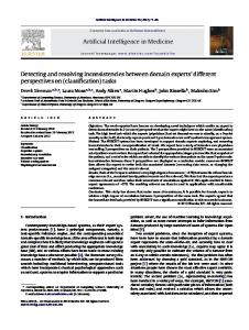
Since df/dx 3 and df/dx 4 differ by only the constant factor 1/m ≤ 1, it is evident that at a maximal point, x3 should be made as small as possible relative to x4 . Therefore x3 = x 4 (1 – 1/m), and again it can be concluded that (3) is the maximum of the nonlinear program. ■ The worst-case performance of Theorem 4.2 with k = 1 is depicted in Figure 4.1. It is interesting to note that this graph is nearly symmetric (to within 5%): f(m, r ) ≈ f (r, m). The asymptotic limiting value along both axes is 2.

There are many important consequences of

33

2 1.8 1.6 1.4 1.2 1 4

4

Dis 3 tan ce M 2 etri c (r )

Performance (W'/W)

2 1.8 1.6 1.4 1.2 1

3

) s (m r o s ces Pro

2 1

Figure 4.1. The performance of AND/OR scheduling according to graph distance.

34

Theorem 4.2. The following Corollary will be used extensively in the remainder of the thesis. If r = 1 and k = 1 then Theorem 4.2 reduces to: Corollary 4.3. If L1 (B(G)) = min{L1 (Bi (G))} then W( B(G))/W opt ≤ 2 – 1/m in any priorityall i

driven schedule of the AND/OR/skipped task system B(G). ■ In the limit as r → ∞ and with k = 1 the performance is Corollary 4.4. If L∞(B(G)) = min{L∞(Bi (G))} then W( B(G))/W opt ≤ 2 in any priority-driven all i

schedule of the AND/OR/skipped task system B(G). ■ If r = 1 and the task system is AND/OR/unskipped, then E*(G) is a constant, hence Corollary 4.5. If L*(B(G)) = min{L*(Bi (G))}, then W( B(G))/W opt ≤ 2–1/m in any priorityall i

driven schedule of the AND/OR/unskipped task system B(G). ■ It is known [Gillies91b] that no AND-only priority-driven algorithm can avoid 2 – 1/m worst-case performance (because priority-driven algorithms never intentionally idle the processor, and sometimes intentional idling is needed). Examples of AND-only task systems that achieve the bound of Corollary 4.5. under any set of task priorities may be found in [Coffman76] and [Gillies91b]. All priority-driven algorithms must schedule these AND-only task systems as a special case. Later in the thesis an algorithm to minimize L*(G) will be presented; this algorithm will be optimal in the sense that it will not be possible to get better worst-case performance from a priority-driven AND/OR/skipped scheduling algorithm. In fact, it has been a long-standing open problem to find a non-priority-driven AND-only scheduling algorithm that avoids 2 – 1/m worst-case performance [Lawler89]. Our last approximation theorem substitutes P*(G) for E*(G) in the distance metric.

35

Theorem 4.6. Define a metric space with axes L*( G) and P*( G)/m. Then if L1 (B(G)) = min{L1 (Bi (G))} then W(B(G))/W opt ≤ 2 in any priority-driven schedule of the AND/OR/skipped all i

task system B(G). Proof. The theorem says that if an AND-only graph B(G) can be found with the property that its longest path and total processing time P*(G) are less than the sum of both quantities in an optimal graph, then the length W(B(G)) of the resulting priority-driven schedule will be at most twice as long as optimal. The proof opens by observing a consequence of Graham's famous theorem [Graham69], namely W(B(G)) ≤ P*(B(G))/m + L*( B(G)). From the assumption that B(G) is a minimal graph, we have P*(B(G))/m + L*(B(G))

≤

P*(Go)/m + L*(Go).

We also observe an obvious lower bound on the length of an optimal schedule, Wopt

≥

max(L*(Go), P*(Go)/m).

From this bound it follows easily that, 2Wopt(Go)

≥

P*(Go)/m + L*(Go),

W(B(G)) Wopt

≤

2. ■

Sometimes there is a choice of graphs B1 (G), B 2 (G), … with Lr (B1 (G)) = L r (B2 (G)) = … ; the next theorem indicates which graph might produce the best schedule. We define the aspect ratio as α = P*(G)/mL*(G). The aspect ratio is a measure of the average utilization in a system with m processors. If α = 1, then the average processor utilization per unit of time is m. If α > 1, then the utilization exceeds m , and if α < 1, then m processors cannot be fully utilized in any schedule. The notion of aspect ratio is taken from the television industry, where a television has

36

an aspect ratio of X/Y if its width is X and its height is Y. Let W denote the length of an optimal schedule and let W' denote the length of a worst-case list schedule. The following theorem relates worst-case scheduling performance to the quantity α. It is a generalization of the theorem of [Graham69]. Theorem 4.7. The worst-case performance of list-scheduling on m processors is

W' W

≤

  

1 1 – α mα 1 1 + α – m

if α ≥ 1 and α m ≥ 1

undefined

if αm < 1.

1 +

if α ≤ 1 and α m ≥ 1

Proof. The time in any list schedule can be divided into two types, known as the idle time and the busy time. Let Wb denote the total length of the busy time and let Wp denote the total length of the idle time. A theorem of [Graham69] states that there is a chain of tasks that executes during the idle time, and that the time is limited by Wp

≤

L*(G)

=

P*(G) / m α.

In a worst-case schedule, at least one task executes during the idle time, and by definition m tasks execute during the busy time, so the worst-case performance of the list schedule is given by the linear program: W' = Wp + W b

maximize subject to

1⋅Wp + mW b ≤ mW

(4)

Wp ≤ P*(G)/mα To solve this linear program observe that W ≥ max(L*(G), P*(G)/m). We change (4) into an equality and solve for intersection points on the surface of the simplex, when Wp = 0 or Wb = 0 or Wp = P*(G)/m α. In the first two cases we arrive at W' = W, but in the third case we obtain W'

= Wp + W b = P*(G)/mα + L*(G)(mα – 1)/m.

We analyze (5) in three cases. 37

(5)

Case 1. α ≥ 1 and αm ≥ 1. Then W ≥ P*(G)/m = α L*(G). Substituting this into (5) we obtain: W' 1 1 ≤ 1 + α – W mα Case 2. α ≤ 1 and α m ≥ 1. Then W ≥ L*(G) = P*(G)/m α. Substituting this into (5) we obtain: W' 1 ≤ 1 + α – W m Case 3. α ≤ 1 and α m < 1. This implies L*(G) > P*(G) which is impossible. The function is undefined. ■ Figure 4.2 depicts the worst-case performance implied by Theorem 4.7. It is interesting to note that if α ≤ .5 or α ≥ 2 then W'/W ≤ 1.5, which is a substantially better guarantee than Graham's original theorem. We believe this theorem might be of use to writers of parallelizing compilers; the theorem may help a compiler to choose between two separate program transformations since the theorem provides an estimate of the worst-case scheduling penalty associated with each transformation. In several simulation studies greedy scheduling has been found to be effective in scheduling a random task system [Biyabani88] [Ramamritham84]. We believe that this conclusion may have been reached because the aspect ratio was not a controlled variable in the simulation. As the theorem above shows, a simulation should generate task systems with α = 1 to ensure that the worst-case workloads are tested. When α = 1 then Theorem 4.7 reduces to W'/W ≤ 2 – 1/m. The worst-case task systems from [Coffman76] and [Gillies91b] both have α = 1. The aspect ratio theorem suggests a method to choose between two different graphs with identical values L1 (B(G)). Presumably, the graphs have different aspect ratios, so one may compute the two worst-case performance levels W'/W from these aspect ratios. Then the

38

0

Proc essor s (m) 8 6 4 2

3 2 (a) 1 Ratio t c e p As

2 1.8 1.6 1.4 1.2 1 4

Performance (W'/W)

10

Figure 4.2. The performance of AND-only scheduling according to aspect ratio.

39

quantity L1 (B(G)) ⋅ W/W' gives an optimistic lower bound on the length of an optimal schedule. The graph with the smaller optimistic lower bound should be chosen. It is likely that the scheduling algorithm will come close to this lower bound. Unfortunately, there are many graphs that achieve the worst-case performance level L1 (B(G)) in all schedules (such as the one in Figure 4.5, which appears later in this chapter). The results of this section are summarized in the following table: Table 4.1. Summary of graph minimization theorems. Theorem

Metric

Space

Task System

Guarantee

4.3 4.4 4.6 4.5

L1 L∞ L1 L1

L*(G), E*(G)/m "" L*(G), P*(G)/m L*(G)

skipped skipped skipped unskipped

2 – 1/m 2 2 2 – 1/m

The remaining sections describe heuristics that exploit Theorem 4.5 or Theorem 4.6. It will be shown that the other metrics mentioned above are more difficult to minimize, hence, no attempt will be made to provide algorithms for these metrics. 4.2. Scheduling to Minimize Completion Time This section presents approximation algorithms to minimize completion time in a multiprocessor. The first subject is an algorithm to schedule AND/OR/unskipped graphs with good worst-case performance. This dispenses with the unskipped scheduling problem for the remainder of the thesis. The rest of the thesis will be concerned with skipped scheduling and different types of precedence constraints. It is shown that the L1 () minimization technique can be applied to AND/OR/skipped intrees, yielding a good approximation algorithm. Unfortunately L1 () cannot be minimized in

40

polynomial time for more complicated graphs; the minimization problem is NP-complete for two types of series-parallel graphs with arbitrary processing times. However, there is an efficient algorithm to schedule generalized series-parallel graphs on a single processor to minimize completion time, and if all the tasks have equal length, there is a fast heuristic to schedule tasks with two-terminal series-parallel precedence constraints on a multiprocessor. 4.2.1. Unskipped Task Systems, Arbitrary Precedence The Minimum Path algorithm selects an AND-only graph which minimizes the quantity L*(B(G)). The scheduling algorithm works as follows.

1.

2.

Input: Threshold graph G = (T, A, P, Π). Output: A schedule of an AND-only graph G = (T, A, P). For each OR task Ti with no OR predecessors: a. Let S be a set of exactly πi direct predecessors of Ti such that the longest path ending at Ti is minimized. In other words, S ⊆ P(G, T i), |S| = π i , and for all Tj ∈ P(G, Ti ) – S and for all Tk ∈ S, L(G, Tj ) ≥ L(G, Tk). b. Convert Ti into an AND task whose direct predecessors are the tasks in set S . The resulting task system G has only AND tasks. Schedule this task system using a priority-driven algorithm and an arbitrary priority list.

Figure 4.3. The minimum path algorithm for general graphs. This algorithm can be implemented to run in time O(n + |A |) by reversing the direction of the arcs in G and employing depth-first search. Let Go = (T o, Ao, Po, Πo) and W o denote the implicit AND-only graph and the completion time of the task system according to an optimal schedule. Let G' = (T', A', P', Π ') and W' denote the AND-only graph and the completion time of the task system according to a schedule produced by the Minimum Path Algorithm, respectively. The worst-case performance of the Minimum Path Algorithm depends on the following lemma. Lemma 4.9. L*(G') ≤ L*(Go).

41

Proof. Let H = {Ti | P(G', T i ) ≠ P(Go, T i )} denote the set of AND tasks whose predecessors differ between the optimal graph and the graph produced in Step 1 of the Minimum Path Algorithm.

If H = ∅ , then the AND-only task graphs are identical and the lemma is

established. Otherwise, let T i ∈ H be an OR task for which there exists no T j ∈ H with T j < Ti in Go. The construction of G ' guarantees that |P (G', T i )| = |P (Go, T i )|.

We assign

A o ← (A o – {(T j , Ti ) | Tj ∈ P(Go, Ti )}) ∪ {(T j , Ti ) | Tj ∈ P (G', Ti )} and obtain no increase in the longest path of Go (by Step 1(b) of the algorithm). This argument is used inductively to transform Go into G' with no increase in the maximum path length. ■ 4.2.2. Skipped Task Systems, In-Trees This section presents a heuristic algorithm to minimize the completion time of an AND/OR/skipped task system with in-tree precedence constraints. The algorithm converts an AND/OR in-tree into an AND-only in-tree that minimizes L1 (B(G)). In a general graph it is difficult to minimize this function quickly. If m = 1, a polynomial-time algorithm to minimize L1 (B(G)) could be used to solve the exact 3-cover problems (refer to Theorem 3.1), implying P = NP. For this reason, the algorithm presented here handles only in-tree task graphs. This algorithm, known as the Path Balancing Algorithm, appears in Figure 4.4. The Path Balancing Algorithm can be implemented efficienctly. The O(n) possible paths from the root to the leaves can be enumerated in time O(n) using a depth-first search. Each iteration of the Steps 1(a) through 1(e) can be carried out together in O(n) time using a recursive depth-first search. Most of the work is done when returning from procedure calls. Hence, the overall complexity of this algorithm is O(n2 ).

This algorithm has been implemented; a

description of the implementation appears in [Sefika91].

42

1.

2.

Input: Threshold graph G = (T, A, P, Π) that is an in-tree. Output: A schedule of an AND-only graph G' = (T', A', P'). For each path C i = {Tx1 < Tx2 < … < Txk} from the root to a leaf in G do begin a. [Copy G] G c ← G. b. [Remove OR tasks from C i] For each task Txj ∈ C i with πj < P(G c, Tj ) set A(Gc) ← (A(Gc) – P(Gc, Txj )) ∪ {(Txj –1 , Txj )} (i.e. make Txj an AND task in Gc). c. [Truncate all paths longer than Ci ] Let C j ≠ C i be a longer path in Gc. If no such C j exists, go to Step (d). Otherwise, let T k be the least task on Cj with P(Gc, Tk) > π k. If no such T k exists then go to Step (g). For each T l ∈ P(Gc, Tk) on a path longer than C i, do begin remove the arc (Tl , Tk) from Gc end. Repeat Step (c). d. [Check for inconsistency] If there is a task Tj with P(Gc, Tj ) < π j, go to Step (g). e. [Minimize processing time] For each task Tk with P(Gc, Tk) > π k which has only AND predecessors in Gc do remove the arc (Tj , Tk) where Tj ∈ P(Gc, Tk) and for all Ti ∈ P(Gc, Tk) with i ≠ j, E(G c, Ti ) ≤ E(Gc, Tj ). f. If the resulting AND-only graph yields an improved value of L 1(G c), record the graph, i.e. G' ← G c . g. end. The resulting task system G' contains only AND tasks. Schedule this task system using a prioritydriven algorithm and an arbitrary priority list.

Figure 4.4. The path-balancing algorithm for in-trees. To derive the worst-case performance of the Path-Balancing Algorithm it is necessary to show that Step 1 of this algorithm minimizes L1 (G'). Lemma 4.10. L1 (G') ≤ L 1 (Go) Proof. Consider the longest path of length L*(Go) in Go This path starts at the tree root and ends at a leaf vertex. Clearly, the Path Balancing Algorithm considers this path in some iteration of Step 1. Step 1(c) of the algorithm ensures that no other paths are longer than this longest path, without increasing E *(G') more than is necessary. Since Step 1(d) of the PathBalancing algorithm chooses the direct predecessors of each OR task to minimize E*(G'), the algorithm cannot fail to find a graph for which L1 (G') is at most E*(Go )/m + L*(Go).■ The example shown in Figure 4.5 demonstrates that this worst-case bound is tight. In the figure, tasks are labeled by their (name, length). For example, (T2 , δ) indicates task T2 requires δ 43

units of processing time. The Path Balancing Algorithm chooses between the two AND-only intrees G 1 = ({T 1 , T2 , T4,1, …, T4, m(m–1)/ ε+1 }, A 1 , P1 , Π1 ) and G 2 = ({T 2 , T3,1, … , T3,m , T5,1, …, T5, m}, A 2 , P2 , Π2 ), where A 1 and A 2 denote the associated arc sets. The lengths of the longest paths in these in-trees are L*(G1 ) = L*(G2 ) = m + δ. Furthermore, E*(G1 ) = E*(G2 ) = m 2 – m. Thus, the Path Balancing Algorithm chooses arbitrarily between these two trees since either one minimizes L1 (G'). There is a schedule of length m + 2δ for G 2 but the shortest possible schedule for G 1 has length m + m(m – 1)/m + δ whenever ε divides (m – 1) evenly. As δ → 0, the ratio of these schedule lengths approaches 2 – 1/m.

(T 1 ,m– ε)

………

{

(T 4,1 ,ε)

G1

(T 4,m(m–1)/ ε + 1 , ε)

(T 2 ,δ) (T 5,1 , m–δ) ………

{

G2

(T 3,1 ,δ)

(T 5,m ,m– δ) (T 3,2 ,δ) ………

(T 3,m ,δ)

Figure 4.5. A worst-case AND/OR/skipped in-tree.

44

4.2.3. Skipped Task Systems, One Processor, Series-Parallel Tasks A series-parallel graph is defined recursively by the following three rules: Notation Rule name

Definition

(1) G = O

singleton rule

G = ({T i }, ∅, {pi }) is a graph consisting of a single task.

(2) G1 |– G 2

series rule

if G1 = (T1 , A1 , P1 ), G 2 = (T2 , A2 , P1 ) then G = (T1 ∪ T2 , A1 ∪ A 2 ∪ T1 × T2 , P1 ∪ P2 ).

(3) G1 || G2 parallel rule

if G1 = (T1 , A1 , P1 ), G 2 = (T2 , A2 , P1 ) then G = (T1 ∪ T2 , A1 ∪ A 2, P1 ∪ P2 ).

Figure 4.6. Rules for a generalized series-parallel graph. A two-terminal series-parallel (TTSP) graph is a graph that always has a distinguished least element and a distinguished greatest element in the partial order, known as the source and sink respectively. The rules for a TTSP graph are based on the operation of identification. Let G 1 and G2 be two graphs with disjoint task sets. The operation of identifying two tasks from different task graphs involves merging the predecessor sets and successor sets for the two tasks and deriving a new task graph with exactly |T(G1 )| + |T(G2 )| – 1 tasks. Notation Rule name

Definition

(1) G = O–O

doubleton rule

G = ({T i , Tj }, {(T i , Tj )}, {p i , pj }) is a graph consisting of two tasks.

(2) G1 |– G 2

series rule

Identify the sink of G1 with the source of G2 .

(3) G1 || G2 parallel rule

Identify the source of G 1 with the source of G2 , and identify the sink of G 1 with the sink of G 2 .

Figure 4.7. Rules for a two-terminal series-parallel graph.

45

The rules above neglect to fully describe the sets P and Π during this process. It is assumed that the task type (AND or OR) is maintained for every subgraph, even if T i does not yet have any predecessors. The algorithms and proofs we present below work only for AND/OR graphs, and not for general graphs, so πi will be irrelevant. It is assumed that when two tasks Ti and T j are identified that pi = pj . Section 4.1 showed that when L1 (B(G)) is minimized, a good heuristic schedule can be produced by any priority-driven scheduling algorithm. The previous section described an algorithm to minimize this function for a AND/OR graph that is an in-tree. In this and subsequent sections, a class of generalized series-parallel graphs is considered. This class contains in-trees as a subclass. It will be shown that for some problems involving series-parallel AND/OR graphs there are polynomial-time approximation algorithms. In other situations the problem of minimizing an AND/OR graph is NP-complete, e.g.: Theorem 4.11. If G is a two-terminal or generalized series-parallel AND/OR/skipped graph, then the problem of finding a graph B(G) that minimizes L∞(B(G)) is NP-complete. Proof. It suffices to show that the problem is NP-complete on a single processor. The proof is based on a reduction from the partition with integer weights problem [Garey79]. Given a set S = {a1 , a 2 , …, an} the problem is to find a partition S = (X, Y) with X ∪ Y = S and X ∩ Y = Ø, such that ∑ ai = ∑ aj (this is known as an equipartition). This problem is NP-complete [Garey79]. ai ∈ X

aj ∈ Y

The partition problem is transformed into a one-processor scheduling problem as follows. Given an input set S, n subgraphs are constructed, one for each a i , as depicted in Figure 4.8(a).

46

(T i,5 , a i)

(T i,6 , a i)

(T i,1 , α) (T i,0 , α)

(T i,4 , a i)

(T i,7 , α)

(Ti,8 , 0 )

(T i,3 , a i)

………………………

(T 0,1 , α)

(T 0,3n , α)

………………………

(T i,2 , α)

(T 0,3n+1 , a 1)

(a) Tasks for weight a i .

(T 0,4n , a n)

(b) Independent task subset.

Figure 4.8. Tasks for an L∞ NP-completeness proof. We connect these subgraphs with an edge (Ti,0, T i+1,7 ) for 1 ≤ i < n. We also add 3n independent tasks (T 0,1, α ), …, (T 0,3n, α ) and n independent tasks (T 0,3n+1 , a 1 ), …, (T 0,4n, a n) as depicted in Figure 4.8(b). Finally, we add two tasks (T0,0, 0) and (T 0,4n+1 , 0) that are not depicted in the figure. T 0,0 has as its direct successors every task in the set {T 1,7, T0,1, …, T 0,4n}, and T0,4n+1 has as its direct predecessors every task in the set {T n,0 , T0,1, …, T 0,4n}. Thus we have formed a task system T = {T0,0, T0,1, …, T0,4n+1 , T1,0, …, Tn,7 }. It should be evident that not only is this a two-terminal series–parallel (TTSP) graph, but it is also a generalized series-parallel (GSP) graph. Suppose there is an answer (X, Y) to the original 2-partition problem. Then if a i ∈ X we include the OR edge (T i,1, Ti,0) in the graph B (G), and if ai ∈ Y then we include the OR edge (Ti,2, Ti,0) in the graph B (G). Then L*(B(G)) = ∑ ai + ( ∑ ai + 3nα ), and E*(B(G)) = ∑ ai + ai ∈ X

all i

ai ∈ Y

( ∑ ai + 3nα ). Hence L*(B(G)) = E*( B(G)). Since ∑ p i,j = K , a constant, no matter which OR all i

Ti,j

edges are chosen in B (G), this choice of arcs is minimum and optimum, and so an optimal algorithm would find an AND-only graph with this cost. Furthermore, it can be seen that from any choice B (G) that minimizes max(L*(B(G)), E*(B(G)) we can derive an equipartition. Hence any algorithm that minimizes L∞(B(G)) can be used to find an equipartition. 47

To prove the theorem for m > 1, for 1 ≤ i ≤ n add tasks Ti,9, … Ti,7+m to the task system, each with predecessor Ti,8 and successor Ti,2 . Also, make m copies of the task subset in Figure 4.8(b) with task labels T 0,1 through T0,4nm.■ The next theorem shows that the minimization problem for L 1 () is nearly as hard as the minimization problem for L∞(). Theorem 4.12. If G is a two-terminal or generalized series-parallel AND/OR/skipped graph then the problem of finding a graph B(G) that minimizes L 1 (B(G)) is NP-complete for m ≥ 2. Proof. Again, the reduction is from partition with a set S of integer weights. First note that the problem can be specialized to the case m = 2. Given a partition problem S we create for each ai the subgraph depicted in Figure 4.9(a) and connect the subgraphs with arcs (Ti,0, Ti+1,8) for 1 ≤ i < n. We also add the independent task that is depicted in Figure 4.9(b). Finally, we add two tasks T 0 and T n+2 (not depicted) and make them the greatest element and the least element in the partial order, respectively. It can be checked that this is both a TTSP and a GSP graph.

a (T i,7 , a i + i) (T i,3 , a i) s

(T i,1 , α) (T i,0 , α)

(T i,4 , a i) (T i,8 , α )

(T i+1,8 , α)

(T i,5 , a i)

(T i,9, 0)

(T i,6 , a i)

(T i,2 , α)

3

1

(T n+1 , 3nα + 2 s + 2 )

(a) Tasks for weight a i .

(b) One extra task.

Figure 4.9. Tasks for an L1 NP-completeness proof.

48

Assume that a scheduling algorithm computes the AND-only graph B(G), including either arc (Ti,1, T i,0) or arc (Ti,2, T i,0) in B(G) for 1 ≤ i ≤ n. Let s = ∑ a i . Let C denote the chain of tasks passing through T i,3 or Ti,4, respectively, for all i. Note that L*(C) ≥ s + 3nα . Let k denote the amount of excess, i.e. k = L*(C) – (s + 3n α). With some thought it can be seen that 0 ≤ k ≤ s + 1. Note that when k = (s + 1)/2 we have L(B(G), T n+1 ) = 3n α + 1.5s + 0.5 and also L*(C) = 3nα + s + k = 3nα + 1.5s + 0.5. Hence L*(B(G))

=

max(L*(B(C)), L*(B(Tn+1 )))

=

max(L*(B(C)), L*(Tn+1 ))

=

max(k + 3nα + s, (s + 1)/2 + 3nα + s).

E*(B(G)) is the remainder of the graph, that is E*(B(G))

min(k + 3nα + s,

=

s+1 + 3nα + s) + … 2

The remaining tasks also include Ti,5 and T i,6 for certain i, and 2⋅[(s+1) – k]⋅s/(s + 1) is the total processing time of the remaining tasks, hence L1 (B(G))

E*(B(G)) 2

=

L*(B(G)) +

=

max(k + 3nα + s, (s + 1)/2 + 3nα + s) min(k + 3nα + s, (s + 1)/2 + 3nα +s) + 2(s – ks/(s + 1)) 2 min(k + C1 , C2 ) ks max(k + C1 , C2 ) + +s– 2 s+1

+ =

s+1 then k + C1 = C 2 and hence 2 C s L1 (B(G)) = C2 + 2 + s – 2 2 s+1 As k increases to + ε we have 2 εs L1 (B(G)) = β + ε – s + 1 s+1 As k decreases to – ε we have 2 ε εs L1 (B(G)) = β – 2 + s + 1 when k =

49

=

β.

>

β.

>

β

which is an increase if s > 1. Hence k =

s+1 is an optimal path length, minimizing L1 (B(G)). But 2

this also corresponds to a partition S = (X, Y) of the two sets: ai ∈ X iff (Ti,1, Ti,0) ∈ A(B(G)) ai ∈ Y iff (T i,2, Ti,0) ∈ A(B(G)).■ Theorem 4.12 does not apply to scheduling on a single processor. In fact, there is a polynomial-time algorithm to compute the optimal schedule of an AND/OR generalized seriesparallel task system for a single processor. To present the algorithm, we start by defining some quantities that it computes.

The quantities are defined for a subgraph H ⊆ G with a

distinguished task T i ∈ H. Ca (H, Ti ) represents the processing time of a chosen AND-only graph H' ⊆ H with every Tj ∈ T(H') obeying Tj ≤ T i . Minimal tasks in H' are allowed to be AND or OR tasks, and Ti is the unique maximal task in H'. Among all the graphs obeying these rules H' is chosen to have the least total processing time. Co (H, Ti ) represents the processing time of a chosen AND-only graph H' ⊆ H with every Tj ∈ T(H') obeying Tj ≤ T i . The minimal tasks in H' are restricted to be OR tasks only, and T i is the unique maximal task in H'. Among all the graphs obeying these rules H' is chosen to have the least total processing time. T

Ca(H) represents the total processing time of a chosen AND-only graph H' ⊆ H. Minimal elements in H' may be AND or OR tasks. All maximal elements of H are included in the graph H'. Among all the graphs obeying these rules H' is chosen to have the least total processing time. T

Co(H) represents the total processing time of a chosen AND-only graph H' ⊆ H. Minimal elements in H' are restricted to be OR tasks only. All the maximal elements of H are included in

50

the graph H'. Among all the graphs obeying these rules H' is chosen to have the least total processing time. The quantities above are defined formally as follows. Ca (H, Ti )

=

Co (H, Ti )

=

T

T

Co(H)

Tj ∈T(B(H)) Tj ≤ T i

B(H), Ti ∈M(B(H))

minimum B(H), Ti ∈M(B(H)) ,

N(B(H)) ⊆To(B(H))

Ca(H)

{ ∑ pj }

minimum

=

{ ∑ pj } Tj ∈T(B(H)) Tj ≤ T i

{ ∑ pj }

minimum

Tj ∈T(B(H))

B(H)

{ ∑ pj } B(H), Tj ∈T(B(H)) N(B(H)) ⊆To(B(H))

=

minimum

If there is no such graph B(H) (i.e. if the result is the empty graph) then the associated T

quantity is defined to be ∞. The goal of a scheduling algorithm should be to compute Ca(G) for the input graph G . The following three lemmas describe a series of rules that can be used to T

T

compute the vector (Ca (H, Ti ), C o (H, Ti ), C a(H), C o(H)) in bottom-up fashion from a seriesparallel decomposition of G: Lemma 4.13. If H = T i is a singleton task then there are two cases. Case 1: Ti ∈ Ta

Case 2: Ti ∈ To

Ca (H, Ti )

=

pi

Ca (H, Ti )

=

pi

Co (H, Ti )

=

∞

Co (H, Ti )

=

pi

T

=

pi

Ca(H)

T

=

pi

T

=

∞

Co(H)

T

=

pi.

Ca(H) Co(H)

Proof. The proof is immediate by the definitions of the vector terms. ■

51

Lemma 4.14. If H = H 1 || H2 and there are minimal vectors for H 1 and H 2 , then the vector for H can be computed as follows. Ca (H, Ti )

=

 Ca (H1 ,Ti)   Ca (H2 ,Ti)

if Ti ∈ H1 if Ti ∈ H2

Co (H, Ti )

=

 Co (H1 ,Ti)   Co (H2 ,Ti)

if Ti ∈ H1 if Ti ∈ H2

T

=

Ca(H1 ) + Ca(H2 )

T

=

Co(H1 ) + Co(H2 )

Ca(H) Co(H)

T

T

T

T

Proof. It should be clear that if H1 and H2 are assembled in parallel then the values for C a() and Co () for H 1 and H 2 are identical to the values for the entire graph H. This is true because the functions Ca (H, T i ) and Co (H, T i ) do not depend on tasks that are not predecessors of Ti ; clearly the parallel composition rule adds no new predecessors to any task T i ∈ H1 ∪ H2 . T

The cost denoted by Ca (H) is the sum of the costs of the subgraphs H 1 and H2 . If this were not the case then there would exist a graph of less cost H' = H'1 ∪ H'2 . But then we would have T

T

T

T

to have either C a(H'1 ) ≤ Ca(H1 ) or C a(H'2 ) ≤ Ca(H2 ), respectively. This would contradict our T

T

assumption that Ca(H1 ) and Ca(H2 ) are minimal. T

A similar argument can be used to show that the rule for Co(H) is correct. ■ Lemma 4.15. If H = H1 |– H 2 and there are minimal cost vectors for H 1 and H 2 , then a cost vector for H can be computed by the following means. First, compute the following minimums for later use. * Ca(H1 ) *

Co(H1 )

← ←

min {Ca (H1 , Ti )}

Ti ∈ M( H1 )

min {Co (H1 , Ti )}

Ti ∈ M( H1 )

Then compute the following values. T

*

T

*

∀Ti ,

Ca (H, Ti )

=

min(Ca(H1 ) + Ca (H2 , Ti ), Ca(H1 ) + Co (H2 , Ti ))

∀Ti ,

Co (H, Ti )

=

min(Co(H1 ) + Ca (H2 , Ti ), Co(H1 ) + Co (H2 , Ti )) 52

(1) (2)

T

T

*

T

(3)

T

T

*

T

(4)

T

=

min(Ca(H1 ) + Ca(H2 ), Ca(H1 ) + Co(H2 ))

T

=

min(Co(H1 ) + Ca(H2 ), Co(H1 ) + Co(H2 )).

Ca(H) Co(H)

Proof. Observe that both H 1 and H 2 are AND-only graphs, except perhaps for a few minimal tasks that may be OR tasks. There are only two ways to affect the total processing time when any two AND/OR graphs are connected in series. Sometimes, H 2 has one or more AND tasks that are minimal; this means that every task in H1 must be executed completely in a schedule. This is represented by the first term in the min() of (1). At other times, H 2 has only OR tasks that are minimal; this allows us to choose a subgraph from H1 to precede the minimal OR tasks of H2 . This situation is represented in the second term in the min() of (1). By an argument similar to Lemma 2, this rule can be shown to be optimal, otherwise there would be a graph H' of lower cost which could be partitioned into two graphs H'1 or H 2' , one of which would have a cost lower than the input cost vector. This would violate the assumptions of the lemma. A similar argument can be used to prove that formulae (2), (3), and (4) produce the correct minimum costs. ■ Theorem 4.16. There is an optimal algorithm to minimize the execution time of an AND/OR generalized series-parallel graph on a single processor. Proof. Apply Lemmas 4.13, 4.14, and 4.15 to the recursive decomposition of the graph. If the n'th application of a lemma minimizes L 1 (H n ), then the (n+1)st application must also minimizes L1 (Hn+1 ). There are at most 2n application of these rules. Hence, in the last step, L1 (B(G)) is minimized and it can be seen that B(G) is a valid AND-only graph that corresponds to the input graph G. ■ The operation of this algorithm can be illustrated with an example. A generalized seriesparallel graph is depicted in Figure 4.10. Tasks are labeled by their (name, processing time).

53

We describe a sequence of composition steps, giving the rule application, the tasks in the graph, and the execution costs in Table 4.2. The series-parallel rules are presented in postfix notation rather than infix to avoid parentheses and to save space in the table. Steps 7, 9, 10, and 11 are abbreviated (applications of rule 1 are omitted) because similar step sequences appear elsewhere in the table. The edges used in the final graph are depicted by dark lines in Figure 4.10. It can be verified that a processing time of 87 is optimal for this input graph.

(T 3 , 25)

(T 9 , 3) (T 7 , 11)

(T 13 , 7)

(T 4 , 27) (T 10 , 4) (T 5 , 29)

(T 15 , 9)

(T 11 , 9)

(T 1 , 4)

(T 14 , 6) (T 8 , 7)

(T 2 , 5)

(T 6 , 12)

(T 12 , 3)

Figure 4.10. Generalized series-parallel task system and its scheduling solution.

54

Table 4.2. The output of an optimal generalized series-parallel scheduling algorithm. Step

Rule

1 2 3 4 5 6 7.… 8 9… 10… 11… 12… 13 14

1 1 2 3 2 3 1,1,2,1,3 2 1,1,2,1,3 1,1,2,1,3 1,1,2,1,3 1,1,2,1,3,2 3 3

Ca (H, Ti ) Co (H, Ti ) CTa(H) T1 {4} {∞} 4 T2 {5} {∞} 5 T1 T2 || {4,5} {∞, ∞} 9 T1 T2 ||T6 |– {16} {∞} 16 T1 T2 ||T6 |–T5 || {16,29} {∞, ∞} 45 T1 T2 ||T6 |–T5 ||T8 |– {52} {∞} 52 T3 T4 ||T7 |– {63} {∞} 63 T1 T2 ||T6 |–T5 ||T8 |–T3 T4 ||T7 |–|| {52,63} {∞,∞} 115 T11T 12||T14|– {9} {15} 9 T9 T10||T13|– {10} {11} 10 T11T 12||T14|– {25} {25} 25 T11T 12||T14|–T9 T10||T13|–|| {9,10} {15,11} 19 T15 and predecessors Ti , i>8 {28} {35} 28 T15 and all predecessors {87} ∞ 87 Graph in postfix notation

T

Co(H) ∞ ∞ ∞ ∞ ∞ ∞ ∞ ∞ 15 11 25 26 35 ∞

We now consider the time complexity of this scheduling algorithm. The generalized seriesparallel graph decomposition can be computed in linear time [Valdes78] [Valdes79]. Lemma 4.13 is applied at most n times and it takes O (1) time to compute the costs for this lemma. Lemmas 4.14 and 4.15 are together applied exactly n – 1 times and they each require O (n) time to update the cost vectors. The step of scheduling the AND-only graph takes O(|A| + n log n) 2

time. Therefore, the complexity of this algorithm is O(n ). 4.2.4. Skipped Task Systems, Two-Terminal Series-Parallel-UET Tasks This section describes an algorithm to minimize the completion time of an AND/OR/skipped task system with UET tasks and two-terminal series-parallel precedence constraints. This type of precedence constraints can be used to model the control flow in a parallel program. By using negative task lengths the algorithm described below may be used to find the maximum execution time of a loopless nondeterministic parallel program. Although we assume TTSP precedence constraints, the TTSP structure need only be present over the OR 55

tasks. AND tasks may form an arbitrary precedence graph as long as those precedence graphs may be collapsed into a single AND task, yielding a TTSP graph. The dynamic programming algorithm works by minimizing L 1 (B(G)) for a fixed value of m. It is possible to extend this algorithm to handle generalized series-parallel precedence constraints, however, the envisioned 4

5

storage requirements (O (n )) and execution time (O(n )) make an extended algorithm impractical for all but the smallest problems. The lemmas that follow may be used to minimize task graph execution time subject to the constraint that no path in the graph has more than k tasks. The following definitions are needed. Let B i,k (G) be a function that maps G onto an AND-only graph where with longest path has at most k tasks. Let C(G, k) = min {P*(B i,k (G))} denote the total execution time of the ANDall i

only graph with no path longer than k tasks. If G is already an AND-only graph, then C(G, k) = P*(G) for k ≥ L*(G), and infinity for k < L*(G). We use the notation G(T i , Tj ) to denote a twoterminal graph with source node Ti and sink node Tj . The algorithm to minimize completion time maintains C(G, k) as follows. Lemma 4.17. If H is a doubleton task pair then C(H, 0) = C(H, 1) = ∞, and ∀i > 1 C(H, i) = 2. Proof. The proof is immediate by the definition of C(G,k). ■ Lemma 4.18. If G = G1 (Ti ,Tj ) || G2 (Ti ,Tj ) and C(G1 , k) and C (G2 , k) are known then C (G, k) may be computed as follows: Case 1: Tj is an OR task

Case 2: Tj is an AND task

C(G, k) = min(C(G1 ,k), C(G2 ,k))

C(G, k) = C(G1 ,k) + C(G2 ,k) – 2.

Proof. If Tj is an OR task then clearly there exist AND-only subgraphs of cost C (G1 , k) and C(G2 , k), and hence C(G, k) ≤ min(C(G1 , k), C(G2 , k)). Since T j is an OR task it must be the case that the graph of cost C(G, k) does not have tasks in both G 1 and G 2 (otherwise these tasks could 56

be deleted, decreasing the cost). Therefore, the graph of cost C(G, k) is either a subgraph of G 1 , or a subgraph of G 2 . Assume without loss of generality that the graph is a subgraph of G1 . Then by the definition of C(G1 , k), C(G, k) ≥ C(G1 , k), hence C(G, k) = C(G1 , k). If T j is an AND task, then there is an AND-only graph Go with minimum execution time that has tasks in both G 1 and G2 . Clearly, C(G, k) ≤ C(G1 , k) + C(G2 , k) – 2. Assume there is a task graph G o with C(Go , k) < C(G1 , k) + C(G2 , k) – 2. Then there must be two subgraphs of G o called G' 1 and G' 2 , with either C(G'1 , k) < C (G1 , k), or C( G'2 , k) < C (G2 , k). This contradicts the assumption that either C(G1 , k) or C(G2 , k) were known to be minimum costs. ■ Lemma 4.19. If G = G 1 |– G 2 and C(G1 , k) and C(G2 , k) are known then the cost of C(G, k) can be computed as follows. C(G, k – 1) = min {C(G1 ,i) + C(G2 ,k – i) – 1} all i

Proof. As in the previous proof, if there is a graph of less cost than C(G1 , i) + C(G2 , k – i) – 1, then it induces a subgraph (assume w.l.o.g.) with longest path length L*(G' 1 ) = l. But then C(G1 , l) ≤ C(G' 1 , l) by definition. Similarly, assume that G' 2 induces a subgraph of length L*(G' 2 ) = λ, then we must have l + λ ≤ k . By the definition of C(G1 , λ), we see that C (G' 1 , λ) ≥ C(G' 1 , k – l), and C(G' 1 , k – l) ≥ C( G1 , k – l), hence we conclude that C(G'2 , λ) ≥ C(G2 , k – l) , thus C( G'1 , l) + C(G' 2 , λ) ≥ C(G1 , l) + C(G2 , k – 1). ■ Theorem 4.20. There is a near-optimal heuristic to minimize the execution time of an AND/OR two-terminal series-parallel graph in a multiprocessor. Proof. Apply Lemmas 4.17, 4.18, and 4.18 to the recursive decomposition of the graph. If the n 'th application of a lemma minimizes C( Gn , k), then the (n+1)st application must also minimize C(Gn, k) for all k. There are at most 2n applications of these rules. Once the vector of costs C(G , k) has been obtained it may be searched for the value of k that minimizes 57

k + (C (G, k) – k )/m. This value of k corresponds to a subgraph B(G) that minimizes L*(B(G)) + E*(B(G))/m. Schedule this subgraph using an arbitrary priority list on a multiprocessor. By Lemma 4.3, the worst-case length of the resultant schedule will be at most 2 – 1/m times optimal. ■ As in the previous section, the TTSP decomposition can be computed in linear time, Lemmas 4.17 and 4.18 are applied at most 2n times at a cost of O(1), and Lemma 4.19 is applied at most n times at a cost of O (n) per application. The time to produce a schedule is O(|A | + 2

n log n). Therefore, the overall complexity of this algorithm is O(n ). The behavior of this algorithm is illustrated with an example. Figure 4.11 contains a twoterminal series-parallel task graph. All the tasks in this graph have length one. Table 4.3 provides the scheduling cost vectors for selected subgraphs of the task graph in Figure 4.11. If the task graph of Figure 4.11 is to be scheduled on 3 processors, then the algorithm would compute C(G(T1 , T7 ), k) for all k and would select the task graph with k = 10; this task graph has a cost of 10 + (21 – 10)/3 = 13.67, which is the least cost for all k on the last row of the table. The selected edges of the graph are outlined with darkened arcs in Figure 4.11. The resultant schedule has length 10, and so the heuristic finds an optimal solution for this example.

T2

T3

T1

T7 T5

T4 T6

58

Figure 4.11. Two-terminal series-parallel task system and its scheduling solution.

Table 4.3. Selected scheduling costs for the TTSP task system. Name of Subgraph C(G(T1 , T2 ), k) C(G(T1 , T4 ), k) C(G(T4 , T6 ), k) C(G(T4 , T5 ), k) C(G(T2 , T3 ), k) C(G(T1 , T7 ), k)

k 10 11 12 13 14 15 16 17

4 5 6 7 8 9 ∞ 6 6 6 … ∞ 11 10 10 10 … ∞ ∞ ∞ 8 8 8 … ∞ ∞ 9 9 9 … ∞ 15 15 13 13 10 10 10 … ∞ ∞ ∞ ∞ ∞ ∞ 21 20 19 18 16 16 16 …

59

CHAPTER 5.

HEURISTIC ALGORITHMS FOR M/SKIPPED TASK SYSTEMS

Chapter 3 showed that the problem of scheduling AND/OR/skipped task systems to minimize completion time is at least as difficult as the set cover problem. In this chapter we propose several heuristics to solve this scheduling problem. The heuristics are generalizations of some of the approximation algorithms in Chapter 4. We also propose a method for generating "difficult" AND/OR scheduling problems, and evaluate the scheduling performance of our heuristics through simulation. 5.1. Generalized Set-Cover Heuristics It was shown in Chapter 3 that the set-cover problem is a special case of the AND/OR/skipped uniprocessor scheduling problem. A good AND/OR/skipped scheduling algorithm should produce good set cover solutions when a bipartite set-cover graph is input to the algorithm. A great deal is known about efficient algorithms for the set cover problem. Adhoc branch-and-bound algorithms have been developed to solve this problem [Fisher90] [Mahanti90]. Cutting-plane branch-and-bound algorithms have also been developed [Balas80a] [Balas80b], and one heuristic with bounded worst-case performance has been developed [Chvatal79] [Lovasz75] [Johnson74]. The algorithms in this thesis are based on a generalization of this last heuristic, which works as follows. Chvatal-Lovasz-Johnson (Clj) Heuristic. The input to this heuristic is a set of vertices V = {v1 , …, vn} , a set of weights W = {w1 , …, wm}, and a set of hyper-edges E = {e 1 , …, em}. Each hyper-edge ej is a subset of V. The algorithm begins with a set E' = Ø and repeats the following 60

two steps until ∪ ej = V: (1) Insert in E' the edge ej that maximizes the cost function|ej | / w j . e j ∈ E'

(2) Delete every vertex in ej from all the other edges in E . The output is a cover E' ⊆ E , and Chvatal has shown that the cost c(E') = ∑

e j ∈ E'

ej wj satisfies c(E') ≤ c(Eopt)⋅ log d, where Eopt is an

optimal cover, and d = max {|ej |}. ■ all j

It is surprising that there is any performance guarantee at all, because the Chvatal-LovaszJohnson heuristic never inspects the hypergraph as it chooses edges. In fact, this worst-case performance occurs even if w j = 1 for all j. Hence, the worst-case performance of the algorithm is likely to arise from the lack of consideration given to the hypergraph structure. In [Balas80b] several closely-related cost functions (such as log|ej | / w j ) were proposed and simulated, and it was suggested that these cost functions might yield better performance than the cost function used by the Clj heuristic. We have disproved this assertion by showing that for any heuristic that inserts edges and for any cost function that is monotone non-decreasing in |ej | and monotone non-increasing in w j , the bound c(E') ≥ c(Eopt)⋅ log d – ε holds for any ε > 0. This knowledge led us to propose some new set-cover heuristics intended to outperform the Clj heuristic. Chvatal-Lovasz-Johnson-Delete (CljDelete). Often the Clj algorithm will produce a cover E' with an edge that is completely superfluous (i.e. every vertex covered by the edge e j is also covered by a different edge in the cover E'). A good implementation should delete these superfluous edges after the Clj algorithm terminates. In fact, any greedy heuristic that inserts edges into a cover can produce superfluous edges, hence a deletion step should be included in every implementation. This is a good reason to design a heuristic around deleting edges from the input set E , rather than inserting edges into a cover E'. There is a second reason why a heuristic designed to delete edges may be simpler to implement. In a threshold graph an OR task is not ready to execute until several predecessors are complete. If the scheduling algorithm

61

operates by deleting edges from the task graph, then it is a simple matter to stop deleting edges when the in-degree of an OR task reaches the threshold πi . On the other hand, if the algorithm inserts edges into the set cover, then it is necessary to write an explicit loop to handle the case where an OR task requires two or more predecessors to begin its execution. For these two reasons, we propose the CljDelete heuristic, which starts with all the edges in the cover E, and then iteratively deletes the edge ej from E which minimizes |ej | / wj . If deleting an edge results in a new vertex vi being covered by only one edge ej = {v j , vj , …, vj }, then ej cannot be deleted 1

2

k

later, and the vertices {v j , v j , …, v j } are removed from the other edges that remain in E. The 1

2

k

algorithm continues until no edge can be deleted from E without uncovering a vertex. The worst-case performance of this algorithm is worse than c(Eopt)⋅ log d, and may be as high as c(Eopt)⋅d; however, in practice this algorithm works about as well as the Clj algorithm.■ Maximum Redundancy Deletion (Mrd). The Mrd algorithm is a refinement of the CljDelete algorithm. Let the degree of a vertex dv (vj ) be the number of edges that cover the vertex vj . Let the degree of an edge de (ej ) = ∑ dv (vi ) be the sum of the degrees of the vertices vi ∈ ej

in the edge. The set cover problem instances that cause Clj to exhibit its worst-case performance often share the same property. When edges of high degree are chosen in the early phases of the Clj heuristic, then worst-case performance is likely to result. If the edges of high degree were deleted first then better performance would often result. The degree de (ej ), divided by the size of the size of the edge |e j | serves as a measure of the degree per vertex covered of ej . This is the basis for the Mrd heuristic. This heuristic is identical to the CljDelete heuristic, except the cost is defined as |de (ej )|⋅wj / |ej |⋅|ej |, and at every step, the highest-cost edge is deleted. ■ Least Independence Deletion (Lid). The Lid heuristic tends to provide optimal solutions for some graphs where the Clj and CljDelete heuristics provide worst-case performance. This heuristic computes a degree of edge overlap that is more refined that Mrd. This overlap

62

measure is called the independence number. The independence number I(e j ) measures exactly the number of edges that overlap edge ej by a given amount. Specifically, let I'(ej , i) = |{e k : |e k∩e j | = i}|, and let I(ej ) = (I'(ej , n), I'(ej , n – 1), …, I'(e j , 0)) be a vector. Independence numbers can be compared lexicographically to find the most redundant edge e j . Thus, the unit cost for the Lid heuristic is defined as I(ej )⋅wj / |ej |⋅|ej |.■ To implement Lid, a vector of geometrically decreasing floating-point numbers 0

1

n

(a , a , …, a ) and the vector I(ej ) is combined with a dot product operator. If a = 1 then Lid and Mrd are the same algorithm. If a = 1/n then the result is an approximation to the lexicographic number I(e j ) with about three significant digits of accuracy if 32-bit floating point numbers are used. This approximation greatly simplifies the implementation of Lid and speeds up its execution. The heuristics above were tested with a preliminary simulation. For the case where wj = 1 and |e j | = 3 for all j, Clj and CljDelete performed equally well; Mrd outperformed Clj and CljDelete; and Lid outperformed all the other heuristics. A three-step process was used to generalize the set-cover algorithms above to schedule AND/OR graphs in a multiprocessor to minimize completion time. In the first step, the setcover algorithms were modified to handle AND/OR graphs where the OR tasks had no successors. In the second step, an outer loop was added so that an AND/OR graph could be processed as a series of modified set-cover problems. This algorithm is sufficient to minimize the execution time of an AND/OR graph on a single processor. To minimize the execution time on a multiprocessor, the length of the longest chain of tasks must be limited in the resultant AND-only graph. The third generalization iteratively reduces the longest chain and calls a uniprocessor algorithm. This generalization will be described in Section 5.3. We now briefly describe the first generalization. The input is a transitively reduced graph G = (T, A, P, Π ), and all the maximal tasks are OR tasks. First the cost of every AND task is 63

computed using the cost functions described earlier in this section. Next, for every direct predecessor T j of an OR task Ti , the costs of the predecessors of T j and Tj itself are summed and associated with T j . For insertion heuristics such as Clj the lowest cost predecessor is chosen and inserted into the final graph. For deletion heuristics such as CljDelete, Mrd, and Lid a search is made among the OR in-arcs for an arc (Ti , T j ) where T i has the highest cost; this arc is deleted from the task graph. The task costs are recomputed and the process is repeated until all the OR tasks become AND tasks. The second generalization works as follows. A subroutine finds all the minimal OR tasks in the graph. Then these OR tasks, together with their AND predecessors, is passed to the generalized set-cover heuristic. When the set-cover heuristic completes, the subroutine is run a second time to find another set of minimal OR tasks, and so on. The implementation was structured to enable recomputation of the set of OR tasks every time an OR task becomes an AND task, however, this frequent recomputation would probably be expensive and would probably not provide much benefit, therefore, this variant was not tested in our simulations. 5.2. Heuristics for One Processor Figure 5.1 contains pseudo-code for the CljDelete heuristic. The generalized set-cover heuristic appears in steps 2 through 8, and steps 0 through 1 and 9 through 10 produce a series of set-cover problems. The operation of this heuristic is illustrated with an example. Figure 5.2(a) depicts an AND/OR graph input to the CljDelete algorithm. The processing time of each task is written next to the task. First the CljDelete algorithm computes the largest possible set of minimal OR tasks (these are depicted in dark grey in Figure 5.2(a)) and restricts its attention to these OR tasks and their predecessors only. Then the CljDelete algorithm counts the number of OR successors for each AND task. This number is divided by the number of OR successors to find a shared processing cost, i.e. 1.5/2 for tasks T2 and T 3; each OR predecessor task will 64

accumulate a shared cost of 0.75. Then each direct predecessor of each OR task is examined. A depth first search is performed and the shared processing cost is summed to get a total processing cost. This total cost is written inside the direct predecessors in the figure. Finally, the task with the highest total cost is deleted from the task graph (this would be T 8 in Figure 5.2(a), causing T11 to be immediately converted into an AND task). When there are no more minimal OR tasks (in this example, when T1 , T4 , and T 8 have been deleted) the result is the task graph of Figure 5.2(b). Then a new set of minimal OR tasks is computed and the procedure repeats itself (T9 is deleted to produce Figure 5.2(c), then T 12 and its unneeded predecessors are deleted to arrive at Figure 5.2(d)). The chosen AND-only graph in Figure 5.2(d) requires six units of processing time, and this is an optimal AND-only task graph for a uniprocessor system. Input: AND/OR graph G = (T, A). set of processing times p[n]. set of task types kind[n]. Output: AND-only graph G = (T, A). Variables: integer length[n], ordegree[n], cost[n], sum[n], dfsmarks[n], unique_id, various queues. 0. Copy the processing time p[] into the array length[]. Initialize an OR_queue with all the least OR tasks in the graph G. 1. If OR_queue is empty, quit (done) 2. Initialize to zero all ordegree[] counters associated w/tasks. 3. For each task T i in the OR_queue a. Choose a new unique_id b. Perform depth-first-search (dfs) using the unique_id to find all the AND tasks T j that are predecessors of T i. Increment the ordegree[Tj] counter of each newly visited AND task. 4. Compute floating-point cost ratio for each AND task Tj: cost[T j] ← length[Tj] / ordegree[Tj] 5. Form predecessor_queue of each direct predecessor of each task in OR_queue 6. For each predecessor task T j in predecessor_queue a. Choose a new unique_id, initialize to zero sum[T j]. b. Perform depth-first search using the unique_id to find all the predecessors Ti of Tj, and compute sum[T j] ← sum[Tj] + cost[Ti ]. 7. Order the predecessor_queue according to decreasing sum[]s computed in step 6. 8. For each task T i in predecessor_queue with maximal sum[T i] a. For each direct OR successor Tj in queue, delete arc (Ti , Tj). If Tj has only one predecessor, remove it from the OR_queue. 9. If the OR_queue is empty then refill the OR_queue with a new set of minimal OR tasks 10. Go to step 1.

Figure 5.1. The CljDelete algorithm for general AND/OR/skipped task systems.

65

The implementation of Mrd is slightly more complicated than the implementation of CljDelete and will be described in detail later. The implementation of Lid is nearly the same as Mrd except the cost computation is even more elaborate. The implementation of Clj is a simplification of CljDelete and is not described here. It was expected that the Lid heuristic would outperform all the other heuristics. Unfortunately, not only was Lid the slowest heuristic of all four, but its performance was much worse than that of other heuristics. This is probably because the initial set-cover simulations were too limited in scope. 1 (T 1, 1)

.75 (T 2, 1.5)

.75 (T 3, 1.5)

2.5 (T 6, 1)

(T 5, 1)

(T 9, 8)

1 (T 4, 1) (T 7, 1)

(T 10, 1)

6

(T 2, 1.5) (T 8, 6)

(T 5, 1)

8 (T 9, 8)

(T 11, 1)

(T 12, 1)

(T 3, 1.5)

(T 6, 1)

(T 7, 1)

7 (T 10, 1)

(T 11, 1)

(T 12, 1) (T 13, 1)

(T 13, 1)

(a) First set-cover problem. (T 2, 1.5) (T 5, 1)

(b) Second set-cover problem.

(T 3, 1.5)

(T 6, 1)

(T 10, 1)

(T 2, 1.5) (T 7, 1)

(T 3, 1.5)

(T 6, 1)

3 (T 11, 1)

(T 11, 1)

6 (T 12, 1)

(T 13, 1)

(T 13, 1)

(c) Final set-cover problem.

(d) Resultant AND-only graph.

Figure 5.2. The cost computation for the CljDelete algorithm. 66

We decided to try to modify the Clj, CljDelete, and Mrd heuristics in an attempt to improve their performance. This was done by improving the accuracy of the costing functions through a process known as mandatory task computation. A mandatory computation finds the set of tasks that must appear in every schedule. This set is derived by adding a new AND task to the graph and making it the successor of every maximal task. Then an AND/OR threshold transitive closure algorithm is used to find the predecessors of this new task.

These

predecessors are mandatory tasks. Because the mandatory tasks must appear in every schedule, we may set the execution time of such tasks to zero so that they do not influence the computation of total execution costs. Figure 5.3 shows a task graph with its transitively reduced precedence constraints depicted by dark arrows; the arcs that would be added by a transitive closure algorithm are depicted by dashed arrows. Tasks found to be mandatory are marked by an "M". Notice that an arc may transit around an OR task in a transitive reduction. This is one of the differences between ANDonly graphs and AND/OR graphs. Special provisions must be made to compute the transitive closure of an AND/OR graph. During the computation, an edge (T i , T j ) with T j ∈ T o may be added to the closure only if there is path from T i to every task in P(G, Tj ). Appendix B describes a fast algorithm to compute the transitive closure of a threshold graph.

M

M

transitive edges intransitive edges Figure 5.3. AND/OR transitive closure. A heuristic such as CljDelete1 runs the mandatory algorithm once to determine mandatory tasks and then sets the execution time of the mandatory tasks to zero. Then the CljDelete 67

algorithm is invoked on the modified graph. This results in improved estimates of the cost of an OR in-arc each time the set-cover algorithm is run.

A heuristic such as CljDeleten

recomputes the mandatory tasks every time an OR in-arc is deleted, resulting in even more accurate savings estimates. The CljDeleten and Mrdn heuristics consistently turned in superior performance. However, these two heuristics were very slow –– probably too slow to be used hundreds of times as needed by our multiprocessor scheduling algorithm. To address this problem we implemented the CljDelete1, Mrd1, CljDelete1Dfs, MrdDelete1Dfs, CljDelete1exp, and Mrd1exp heuristics. The CljDelete1dfs (depth-first-search) heuristic is a poor-man's implementation of CljDeleten; the mandatory algorithm is run once at the beginning, but later a fast depth-first search is substituted for the mandatory algorithm. The mandatory algorithm 3

takes O(n ) time, whereas the depth-first search takes linear O(n + |A |) time.

The

CljDelete1exp (experimental) marks a task "needed" if there is one OR task with the task as its sole direct predecessor. This causes the set-cover heuristic to realize that a "needed" task cannot be deleted from the graph (at least for the particular set-cover problem). Both the "exp" and the "dfs" heuristics were designed to give optimal performance when a set-cover problem corresponding to the cycle graph C6 was input. In total there were 5 variants each of CljDelete and Mrd. We list the changes made to CljDelete to produce these variants in Figures 5.4 through 5.8. 2. 3.

4.

Initialize to zero all ordegree[] and coverdegree[] counters associated w/tasks. For each task T i in the OR_queue a. Choose a new unique_id. covercost ← |P(G, T i)| b. Perform depth-first-search (dfs) using the unique_id to find all the AND tasks T j that are predecessors of T i. Increment the ordegree[Tj] counter of each newly visited AND task. Increment the coverdegree[Tj] counter by covercost. Compute floating-point cost ratio for each AND task Tj: cost[T j] ← length[Tj] * coverdegree[T j] / ordegree[Tj] * ordegree[Tj]

Figure 5.4. Code revisions for Mrd.

68

0.5.

Run the mandatory closure to find mandatory tasks. Set length[T i] ← 0 for each mandatory task.

Figure 5.5. Additional code for [heuristic]1. 2.5.

Run the mandatory closure to find mandatory tasks. Set length[T i] ← 0 for each mandatory task.

Figure 5.6. Additional code for [heuristic]n. 8.b.

If OR task Tj now has only one predecessor, do a dfs to set the cost[] of every task that is a predecessor of T j to zero.

Figure 5.7. Additional code for [heuristic]dfs. 5. 5.5.

For each OR task from OR_queue with only 1 predecessor, mark the predecessor "needed" Form predecessor_queue of each direct predecessor (that is not "needed") of each task in the OR_queue.

Figure 5.8. Code revisions for [heuristic]exp. In addition to the changes listed above, only Clj, CljDelete, Lid, and Mrd perform the loop over T j as described in step 8 above.

All the other heuristics (Clj1, Cljn, CljDelete1,

CljDelete1Dfs, CljDelete1exp, CljDeleten, Mrd1, Mrd1Dfs, Mrd1exp, and Mrdn) are limited to one iteration of the loop before they fall through to step 9. This change produces optimal performance from these heuristics on the cycle graphs C n . The Clj, CljDelete, Lid, and Mrd algorithms are faster because they attempt to remove several OR predecessors from the graph at once, however, for some graphs it is more prudent to recompute task costs after every OR predecessor is removed. By recomputing task costs frequently the algorithms can make a more informed decision about which arc to remove next. It can be seen that the Clj, CljDelete, Mrd, and Lid heuristics are strict generalizations of the algorithms presented in Section 5.1. If a bipartite task graph is fed to these algorithms, then they behave exactly the same as the corresponding set-cover algorithm with an equivalent set-

69

cover problem. It can also be seen that these algorithms minimize P*(B(G)) for in-trees and are optimal for a single processor. Table 5.1 lists these algorithms in order of increasing complexity, where n is the number of tasks in the task system, and m = |A| is the number of arcs in the task graph. Table 5.1. Algorithm complexity. Algorithm Clj, Clj1 Mrd, Mrd1, Mrd1Dfs, Mrd1Exp, CljDelete, CljDelete1, CljDelete1Dfs, CljDelete1Exp Cljn Mrdn, CljDeleten, Lid

Worst-case Complexity 2

O(n (m + n)) O(mn(m + n)) 4

O(n ) 3 O(mn )

5.3. Heuristic Extensions for a Multiprocessor Figure 5.9 presents an algorithm to shorten the longest chain in a graph. The basic operation begins with a step that identifies a longest path in an AND/OR graph G. A copy G 2 of the graph is made and any OR tasks along the longest path are converted to AND tasks in G2 . A subroutine is called to minimize the uniprocessor execution time of G 2 . The resultant ANDonly graph is measured to see if it its worst-case performance is smaller than any previous version of G 2 . If it is smaller then G 2 is recorded as the best graph found so far. Then, the longest path in G is broken by removing a single OR in-arc and the whole algorithm repeats. The algorithm terminates when it finds a longest path that consists solely of AND tasks, since such a path cannot be shortened. The idea for the algorithm is simple, however, problems arise when there are several longest paths of the same length. Most of the complexity in the algorithm is needed to handle this special case. With some thought it can be see that this is a refinement of the minimum path algorithm from Section 4.2.1 of this thesis. The Shorten() algorithm runs in at most O(|A|) iterations and 70

induces one longest path in time O(|A|). In the very last iteration the algorithm has done the

Input: AND/OR graph G = (T, A). processing times p[n], task types kind[n], subroutine name H() Output: AND/OR graph G = (T, A) passed several times to H() Variables: integer L, or_queue[], arc_queue[], M[]; graph G 2; A. Copy input graph G 2 : = G. Record maximum tasks of G 2 in a set M. B. Repeat 1. For each arc in G 2 compute the length of the longest path going through that arc. 2. Compute length L of longest path in G2. 3. Identify all arcs (T ik–1 , Ti k) in G 2 such that: a. A path (T i1 , Ti 2 , …, Ti k) exists with each arc on a path of length L. b. Ti 1 , …, Ti k-1 are all AND tasks c. Ti k is an OR task Store each (Ti k–1 , Ti k) in arc_queue and arc_queue2. 4. Repeat a. Copy AND/OR graph: G ← G2. b. If arc_queue is non-empty Dequeue arc A 0 = (T i, Tj) from arc_queue. Forever do Install Ti as sole direct predecessor of T j in G. Follow any longest path from Tj until we encounter (a) a new arc A 0 = (T i, Tj) with T j an OR task. Continue forever loop. (b) a greatest task (end of path). Exit forever loop. end c. Call set-cover heuristic H(G). d. Record cost of solution. Until (arc_queue is empty) 5. For each arc (Ti , Tj) in arc_queue2 a. If Tj is an OR task in G 2 with only one predecessor, convert T j to an AND task in G 2. Else delete the arc (Ti , Tj) from G 2. 6. Detect all tasks no longer reachable from any task in M in G 2; set their lengths to zero in G2. Until (no more minimum OR tasks in G2)

Figure 5.9. The Shorten() algorithm for general AND/OR/skipped task systems. same work as the minimum path algorithm, i.e. it minimizes L*(B(G)). Therefore, Shorten() has 2 – 1/m worst-case performance for AND/OR/unskipped task graphs in a system with m processors. It is not difficult to check that Shorten() together with any of the uniprocessor scheduling algorithms mentioned previously will minimize L1 (B(G)) for an in-tree in a

71

multiprocessor system. Thus, all the heuristics in this chapter have 2 – 1/m worst-case performance for in-trees in a multiprocessor system. A graph such as an in-tree has a linear number of longest paths. Shorten() enumerates every longest path in an in-tree, and also samples every longest path in a bipartite digraph. There are probably many other types of graphs for which this algorithm examines every longest path. For these graphs, if the uniprocessor scheduling algorithm provides a performance guarantee, then the entire algorithm would provide a heuristic performance guarantee as given by Theorem 4.2. 5.4. Simulation Parameters This section describes two methods for generating random AND/OR graphs. These methods were designed with two things in mind: (1) to create a graph that was hard to schedule, utilizing knowledge learned in the analysis of the AND/OR scheduling problem; and (2) to be easily parameterized and easily implemented. Since the set-cover heuristics of this thesis have a wide range of worst-case performance levels (from log n to n times optimal), it is important to generate problems that could exercise this worst case performance. To find a class of graphs with worst-case performance it is necessary to control the graph generation algorithm carefully. Thus, the graph generation algorithm has a rich set of parameters: Random Seed r . The simulation was written to make every graph a function of its parameters and its random seed. To make the software portable and repeatable, a 32-bit linear congruential random number generator was used (it was borrowed from the Macintosh LightspeedC development environment). Edge Probability q. To install graph edges each task T i and task T j with j > i is examined, and with probability q the arc (Ti , Tj ) is installed in the random graph.

72

Grid Ratio X/Y. It is important to generate graphs with many incomparable tasks and with longest paths of limited length, since these parameters greatly influence the difficulty of a particular problem instance. The method used is similar to the techniques used to generate network flow problems. The tasks of the graph are laid out on a grid of Y rows and X columns. An arc may exist only between a task on row i and row i+1 or greater. This guarantees that there are at least X incomparable tasks in every row of the graph, and it also guarantees that the longest path has at most Y tasks. A graph is said to have grid ratio X/Y if it is generated with an X by Y grid. Task processing time distribution interval [a, b]. The processing time of a task is a random integer-valued variable drawn uniformly from the range [a, b]. Percentage of OR Tasks p. Every task with two or more predecessors can potentially be an OR task. However, if every such task is made an OR task then the resultant graph would resemble a tree; many OR tasks would occur near the minimal tasks in the graph and chains of AND tasks would appear elsewhere. After a graph is generated, the number of AND tasks with two or more predecessors is computed and then it is multiplied by the factor 0 ≤ p ≤ 1 to determine the number of OR tasks to generate. OR Task Generator (ToughOr or EasyOr). The procedure for constructing a "tough" random graph is depicted in Figure 5.10. This algorithm is intended to make almost the entire graph optional. It can be observed that step (6) always starts by converting the maximal tasks into OR tasks (if possible). Later, predecessors discovered by the mandatory algorithm are converted into OR tasks. If a sufficient number of OR tasks are requested, the resulting graph has almost no mandatory tasks; only a handful of OR tasks in several groups are mandatory. This makes it likely that most of the graph can be eliminated by a clever AND/OR scheduling algorithm.

73

1. 2. 3. 4. 5. 6.

Input: parameters r, q, X, Y, a, b, p. Output: task graph G = (T, A, P, Π ). Seed the random number generator. Generate an AND-only graph G on an X by Y grid with edge probability q, and integer task lengths chosen randomly and uniformly in the range [a, b]. Perform transitive reduction on G . Compute k , the number of potential OR tasks (with two or more predecessors) in G. Initialize a random number generator that selects tasks without replacement. Run the mandatory algorithm and mark every task either "mandatory" or "optional". Compute a subset S of tasks (potential OR tasks) as follows Each task in S must (a) be an AND task, (b) have indegree ≥ 2, and (c) be mandatory and have no mandatory successors. If S = Ø , then make every AND task with in-degree greater than two a member of S. Select tasks from S until (a) exactly k⋅p OR tasks have been selected, or (b) the set S is exhausted. If S is exhausted, then repeat Step 6.

Figure 5.10. The ToughOr task graph generation algorithm. It may seem that step (6) is overly complicated or unnatural, however, we believe it is necessary. An EasyOr task generator was also implemented that chooses OR tasks randomly from the set of AND tasks with in-degree greater than two. When OR tasks were selected in this way, the average difference between shortest schedule and the longest schedule on a single processor was only 6% of the total schedule length (over a series of 135 experiments, and all the data points), and the maximum difference was 35%. The difference was small because the EasyOr task generator tends to make the entire graph mandatory, hence, the heuristics cannot find a radically simplified AND-only graph. With the ToughOr task generator of step (5) above, the average difference was 26%, and the maximum difference was 108%. 5.5. Simulation Results All fourteen algorithms described in the previous section were implemented in ANSI C and debugged on both Macintosh and UNIX computers. Each heuristic required about 100 lines of C to implement; the entire software system comprised approximately 4000 lines of active code. Three sets of simulations were run on the heuristics. First of all, the heuristics were tested on in-trees and it was verified that all 14 heuristics minimized L 1 (B(G)) when G was a tree.

74

Second, a set of coverage experiments was run to get an idea of how the heuristics performed on a broad range of inputs. An algorithm known as Random(1000) was developed to provide a baseline for comparison.

This algorithm generated 1000 solutions to the

uniprocessor scheduling problem and chose the best solution. If there were 1000 or fewer possible AND/OR graphs then the algorithm simply enumerated every possible solution. It was found that this optimization made the randomized algorithm run much faster on small problems without significantly changing the quality of random solutions. An unoptimized algorithm tended to diverge from the random(1000) algorithm only when the number of possible graphs was in the range [500,1000], and this occurred only for a fraction of one data point in each simulation run. Next the 15 heuristics (including the random algorithm) were run on a copy of the same graph, a solution was recorded for each heuristic; and the solution was divided by the size of the random solution to get a performance ratio. These performance ratios generally fell in the range [.4, 1.2], i.e. the heuristics produced schedules that were anywhere from 40% to 120% of the length of the solution from the random(1000) scheduler. A total of 270 combinations of simulation parameters were developed. These parameters are listed in Table 5.2. Two hundred and seventy simulation processes were run to provide adequate coverage for the parameters of the graph generation algorithm. The given grid ratios restricted the number of tasks in a graph to a small set of values and all possible values for n ≤ 200 were tried (except for an grid ratio of 1, for which n ≤ 150 was used). For each number of tasks at least ten random graphs were generated and scheduled by all 15 algorithms. Almost immediately it became apparent that the Lid algorithm was going to be the most expensive algorithm and also the algorithm with the worst performance, so no attempt was made to extend this algorithm to get Lid1, Lid1Dfs, Lid1Exp, or Lidn algorithms.

75

Table 5.2. Simulation parameters. Edge Probability Permutation OR Fraction Task Length Grid Ratio

.1 Tough .2 [1, 1] .2

.5

.9 Easy

.5

.5 [1, 10] 1

.8 [1, 100] 2 5

For each of the 270 coverage runs and for each heuristic, a performance level was computed as the sum of each data point (from 6 to 12 data points) in the given run. This yielded 14*270 performance numbers. For each simulation the variance in performance levels was computed and used to determine "interesting" simulations, i.e. those simulation that discriminated the most between the different heuristics.

Lid was not included in the performance level

computation since it was not a promising algorithm and because it tended to obscure the differences between the other algorithms. Because of the difficulty of plotting 13 algorithms on a single graph, only Mrd, Mrd1, Mrd, Clj1, CljDelete1, and Lid were plotted. Mrdn and CljDeleten almost always turned in identical performance. The Dfs and Exp heuristics were found to work well mainly when the task length was in the interval [1,1], hence, they performed poorly in the majority of the simulations. Nine simulations from the 270 coverage runs were chosen for further study. These were run asking for a 90% confidence level and intervals of width .004 obtained in not less than 10 and not more than 1000 trials. The Random(1000) algorithm was replaced with a Random(100,000) algorithm which was extraordinarily slow. Almost without exception, the confidence intervals did not decrease below .004 for all 15 algorithms, and 1000 trials were run for every data point. The nine simulations are listed in Table 5.3.

76

Table 5.3. Simulation trials reported in this thesis. Distinguishing Feature variance variance variance variance variance complements 1st, 3rd slowest convergence unit length typical workload

Var. Rank 1st 2nd 3rd 5th 6th 19th 21st 28th 116th

Trial #104 #95 #103 #239 #243 #102 #112 #66 #209

Permutation Tough Tough Tough Easy Easy Tough Tough Tough Easy

OR fract. p 0.8 0.8 0.8 0.8 0.8 0.8 0.8 0.5 0.5

Grid Ratio X/Y .5 .2 .5 .5 1 .5 1 1 2

Edge prob. q 0.5 0.5 0.5 0.5 .1 0.5 0.5 0.5 0.1

Task Length [a, b] [1, 100] [1, 100] [1, 10] [1, 100] [1, 1] [1, 1] [1, 10] [1, 1] [1, 100]

Best Performance. The 14 heuristics can be ranked into performance groups according to our initial run of 270 simulations. The groups are, approximately, {Mrdn, CljDeleten}, Cljn, Clj1, {Mrd1, CljDelete1}, {CljDelete1Exp, Mrd1Dfs, Clj, Mrd1exp}, {Mrd, CljDelete}, Lid, Random(1000). The overall performance levels are presented in Table 5.4. Each table entry is the sum of 1744 data points taken in the 270 trials, with 6-12 data points per trial (632 uninteresting data points were omitted because at these points all the algorithms were optimal). The surprising fact from this ranking is the good performance of Clj1. Clj1 is one of the fastest heuristics implemented but its performance was only 1.3% worse than the two best heuristics, Mrdn and CljDeleten. In general, the Mrd heuristics performed surprisingly well. They tended to outperform the related CljDelete heuristics by a small margin, and both tended to outperform the Clj heuristics.

This validates our attempt to improve upon the standard set-cover

algorithms. The results of the simulations are depicted in Figures 5.11-5.15. For each graph and for the first few data points (n ≤ 50), the Random(100,000) algorithm enumerated every possible graph and found the optimal solution. The range where Random(100,000) was optimal is depicted by shading the left side of these graphs. The individual simulation runs are described next.

77

Table 5.4. The overall performance of the 14 heuristics Heuristic Name Mrdn CljDeleten Cljn Clj1 Mrd1 CljDelete1 CljDelete1Dfs CljDelete1exp Mrd1Dfs Clj Mrd1exp Mrd CljDelete Lid Rand(1000)

Total Performance 1485.04688 1485.90119 1492.27433 1510.8398 1522.11913 1524.41549 1525.75415 1533.40659 1533.79386 1544.96459 1546.56637 1559.49036 1561.02613 1685.08333 1744

Highest Variance. Simulation #104 (Figure 5.11) exhibited the highest algorithm variance among all the simulations. In other words, this simulation yielded the highest distinction between the algorithms. In this simulation, Mrdn and CljDeleten (not depicted) turned in nearly indistinguishable performance, with Cljn (not depicted) close behind. It can be seen that Clj1 ran a distant 4th in this simulation. Simulation #95 (Figure 5.11) depicts the run with the second highest variance. The only difference is that the grid ratio is .2, rather than .5. For completeness, two other simulations closely related to Simulation #104 are depicted in Figure 5.12. Simulation #103 had the third highest variance of all the heuristics. This simulation differs from #104 only in that the task lengths are chosen from the interval [1,10] rather than [1,100]. Simulation #102 was included so that the reader could see effect of task length on the performance of the heuristics. Simulations #102, #103, and #104 are all equivalent except that task lengths are chosen from the interval [1, 1], [1, 10], and [1, 100]. Apparently, more variance in the task length leads to more variance in the simulation outcome.

78

1.6

Simulation #104

1.2

1.0 Optimal Range

Heuristic Performance

1.4

0.8 0.6

Mrdn Mrd1 Mrd Clj1 CljDelete1 Lid

0.4 0

50

1.6

100 Tasks

150

200

100 Tasks

150

200

Simulation #95

1.2

1.0 Optimal Range

Heuristic Performance

1.4

0.8 0.6

Mrdn Mrd1 Mrd Clj1 CljDelete1 Lid

0.4 0

50

Figure 5.11. Simulations with the highest variance. 79

1.6

Simulation #103

1.2

1.0 Optimal Range

Heuristic Performance

1.4

0.8 0.6

Mrdn Mrd1 Mrd Clj1 CljDelete1 Lid

0.4 0

50

1.6

100 Tasks

150

200

100 Tasks

150

200

Simulation #102

1.2

1.0 Optimal Range

Heuristic Performance

1.4

0.8 0.6

Mrdn Mrd1 Mrd Clj1 CljDelete1 Lid

0.4 0

50

Figure 5.12. The effect of differing task lengths. 80

Slowest Convergence. Simulation #112 converged more slowly than any other simulation. In other words, during the coverage experiment the confidence interval software asked for the greatest number of trials for this combination of graph parameters. This simulation is depicted in Figure 5.13. In fact, for 4 out of 8 data points in the coverage run one hundred trials were generated because the confidence did not decrease to a value below .002. Thus, we feel this combination of graph parameters yielded the most unstable performance. This may have happened for two reasons. First, 80% of the potential tasks are OR tasks, so the actual number of OR tasks varied widely for each data point, depending upon the number of potential OR tasks. And second, the grid ratio was 1 so the graphs produced could form a sequence of difficult set-cover problems. In fact, Simulation #111 (identical except tasks lengths chosen in the interval [1,1]) and Simulation #113 (identical except task lengths chosen in the interval [1,100]) called for the second and third slowest convergence. Clearly, this combination of input parameters led to high variance in heuristic performance (as measured by the number of trials) no matter what the task lengths were. Predicted Highest Variance. A priori of the experiments, Simulation #66 was expected to exhibit the highest variance (refer to Figure 5.13). This is because it was thought that a graph with medium edge density and a grid ratio of 1 would be the hardest to schedule. It turned that Simulation #66 was 27th in variance. However, the top 26 simulations had an OR fraction of 0.8, and #27 had the highest variance among simulations with an OR fraction other than 0.8. EasyOr Task Permutation. Simulation #209 uses the EasyOr task generator and is typical of simulations with this generator. For this simulation, depicted in figure 5.14, the heuristics performed very well because the problem was too easy. In fact, it is difficult to determine which heuristic is best for nearly all of the simulations that used the Easy permutation generator. In general, the problems generated by the EasyPerm OR task generator were not as

81

1.6

Simulation #112

1.2

1.0 Optimal Range

Heuristic Performance

1.4

0.8 0.6

Mrdn Mrd1 Mrd Clj1 CljDelete1 Lid

0.4 0

50

1.6

100 Tasks

200

Simulation #66 Mrdn Mrd1 Mrd Clj1 CljDelete1 Lid

1.4 1.2

1.0 Optimal Range

Heuristic Performance

150

0.8 0.6

0.4 0

50

100 Tasks

150

200

Figure 5.13. Simulations with slow convergence or predicted poor performance. 82

Simulation #209 Optimal Range

1.06

Heuristic Performance

1.05 1.04 1.03

Mrdn Mrd1 Mrd Clj1 CljDelete1 Lid

1.02 1.01 1.00 0.99 0.98 0

50

100 Tasks

1.4

150

200

Simulation #239

1.0

Optimal Range

Heuristic Performance

1.2

0.8

0.6

Mrdn Mrd1 Mrd Clj1 CljDelete1 Lid

0.4 0

50

100 Tasks

150

200

Figure 5.14. Simulations using the Easy OR task generator.

83

challenging as those generated by the ToughOr task generator. Simulation #239 had the highest variance among all the simulations with the EasyOr task generator. This simulation differs from Simulation #104 only in the choice of permutation generator. Simulation #243 (Figure 5.15) had the second highest variance among the simulations with the EasyOr task generator, and the 6th highest variance overall. It is interesting to note that the grid ratio of 1 and the edge probability of .1 and the task length of [1, 1] is very unusual among the simulations with high variance. Speed of Execution. The 9 simulations depicted in Table 5.3 were instrumented to measure execution time. Figure 5.16 plots the execution time as a function of the input graph size at a 90% confidence level. The algorithm speeds fell into two categories: Simulations {95, 102, 103, 104, 112, 239, 243} and Simulations {66, 209}. Simulations #103 and #209 were chosen as representatives of their categories; the other graphs are virtually indistinguishable from these two. It can be seen that the speed of the Clj1 heuristic is nearly identical in both simulations (ending at .2 seconds for 200 tasks). This is because the heuristic depends mainly on the number of OR tasks in the input graph and because one call to the Mandatory() algorithm can take as much as 30% of the total processing time. On the other hand, the heuristics Mrd, Mrd1, and CljDelete1 ran more slowly in Simulations {66, 209} than in simulations {95, 102, 103, 104, 112, 239, 243}. This is because both the input graphs and output schedules from Simulations #66 and #209 had more AND tasks than in the other simulations. The Mrd, Mrd1, and CljDelete1 algorithms have to compute the cost of all the AND tasks every time an OR in-arc is deleted; a great number of AND tasks causes great amounts of time to be spent in recomputing subgraph costs.

84

1.4

Simulation #243

1.0

Optimal Range

Heuristic Performance

1.2

0.8

0.6

Mrdn Mrd1 Mrd Clj1 CljDelete1 Lid

0.4 0

50

100 Tasks

150

200

Figure 5.15. Simulations using the EasyOr task generator, second in variance.

85

0.5

Simulation #209 Mrdn Mrd1 Mrd Clj1 CljDelete1 Lid

Mean time in seconds

0.4

0.3

0.2

0.1

0.0 0

0.5

50

100 Tasks

200

Simulation #103 Mrdn Mrd1 Mrd Clj1 CljDelete1 Lid

0.4 Mean time in seconds

150

0.3

0.2

0.1

0.0 0

50

100 Tasks

150

200

Figure 5.16. The execution time of the uniprocessor scheduling algorithms.

86

Multiprocessor Scheduling.

The Shorten() algorithm was implemented to facilitate

multiprocessor scheduling. This algorithm shortens the longest path of an AND/OR task graph by a minimal amount and then calls a uniprocessor AND/OR/skipped scheduling heuristic on the resulting graph. Shorten() terminates when no further shortening is possible and may be used in conjunction with any of the 14 algorithms described above, or no algorithm at all. Shorten() was found to work well with the heuristics described above, however, it was not tested extensively because it multiplied the time complexity of an algorithm by O(|A|) yielding a substantial time penalty. Furthermore, no alternatives to Shorten() were developed so there were no other multiprocessor algorithms available for comparison. Judging from the earlier simulation results, we recommend that the Shorten() algorithm be used together with the Mrdn or CljDeleten algorithms. If execution time is critical, the faster Clj1 algorithm could be run in conjunction with Shorten(). The Clj1 algorithm ran about n times faster than Mrdn and CljDeleten algorithm in the simulations, and produced results of nearly the same quality.

87

CHAPTER 6.

RELATED WORK

This chapter contains a review of some previous work that is related to the AND/OR scheduling problem. It is believed that the task model developed in this thesis has not been considered in any previous publications; hence there is no directly relevant previous work. Therefore, most of this chapter describes the work in scheduling that is closest to the work in this thesis. The chapter also discusses related subjects such as the transitive closure problem on directed graphs. 6.1. Scheduling to Meet Deadlines The problem of scheduling tasks with release times and deadlines has been extensively studied. In the case where there are no precedence constraints, arbitrary execution times, and preemption is allowed, the earliest deadline first method has been shown to be optimal for a single processor [Liu73]. In other words, if there is a schedule that meets all the deadlines then the earliest deadline first rule finds such a schedule. The least-laxity-first algorithm is also optimal, but it can lead to an inordinate number of preemptions [Dertouzos74]. When there are several processors McNaughton's algorithm can be used to meet multiple deadlines. If preemption is not allowed then the problem is NP-complete, even for a single deadline, but if all the tasks have identical execution times (UET tasks) then the algorithm of [Simons83] can be used to meet integer release times and deadlines. When the release times and deadlines are arbitrary rational numbers, then it is possible to meet deadlines for UET tasks on a single processor [Garey81]. 88

When precedence constraints are present in a uniprocessor task system then a deadline modification algorithm can be used to remove these constraints [Garey76] (see Section 2.3). Therefore, precedence constraints are usually not a problem in scheduling a uniprocessor. When precedence constraints are present in a multiprocessor system and the tasks are UET, then the algorithms [Garey76] [Garey77] can be used to meet deadlines or to meet release times and deadlines on two processors. When the precedence constraints form an in-tree and the tasks are UET, then there is an optimal algorithm to meet deadlines on a multiprocessors [Hu61]. The earlier work in scheduling to meet deadlines provides a multitude of tractable ANDonly scheduling problems. These problems were investigated in Chapter three to see if the corresponding AND/OR scheduling problems could be solved in polynomial time. 6.2. Scheduling to Minimize Completion Time A widely studied problem is that of scheduling unit-execution-time tasks with precedence constraints to minimize completion time on two processors. Many algorithms have been proposed to solve this problem [Fuji69] [Muraoka71] [Coffman72] [Garey77]. When a third processor is present, the complexity of the problem is unknown and has remained one of the most famous open problems in complexity theory [Garey79]. For an arbitrary number of processors, three heuristics have been analyzed. Graham showed that for tasks of arbitrary length and with arbitrary execution time, all schedules obey the bound W'/W ≤ 2 – 1/m, where m is the number of processors, W' is the length of a worstcase schedule, and W is the length of an optimal schedule [Graham69]. Chen and Liu [Chen75] showed that for UET tasks and the longest-processing-time (LPT) algorithm, W'/W ≤ 2 – 1/(m – 1) for m ≥ 3, and W'/W ≤ 4/3 for m = 2. Coffman and Graham 89

examined an algorithm that is a refinement of LPT, and showed that it was optimal for 2processor scheduling [Coffman72]. Lam and Sethi extended this proof to show that the algorithm obeys the bound W'/W ≤ 2 – 2/m for an arbitrary number of processors [Lam77]. Gillies [Gillies93a] has analyzed the algorithm of [Garey76] in the context of m -processor scheduling. He showed that W'/W ≤ 2 – 2/m for m ≠ 3, and W'/W = 3/2 for m = 3. When preemption is allowed and the task lengths are arbitrary, Muntz and Coffman proposed an algorithm that is optimal for two processors [Muntz72]. Lam and Sethi extended this algorithm to show W'/W ≤ 2 – 2/m when an arbitrary number of processors are present [Lam77]. Many researchers have considered the problem of scheduling with additional constraints such as resources or processors of different speeds. The most relevant work along these lines is our own; it introduce a method of finding the worst-case heuristic performance using symbolic linear programming [Gillies89] [Gillies91b]. The work in this thesis builds mainly on the work of Graham. As was shown in Chapter 4, the distance measures used in this thesis are NP-complete to compute, even for generalized series-parallel graphs and arbitrary execution times. Some day a distance measure might be developed that would allow the Coffman-Graham algorithm to provide a performance guarantee of 2 – 1/m for AND/OR/skipped UET task systems with in-tree precedence constraints. 6.3. Scheduling Parallelizable Jobs Recently there has been growing interest in the problem of scheduling jobs with a variable amount of parallelism. In this problem it is assumed that each job has a unique parallel speedup si and that each job may execute using anywhere from one to m processors. If a job 90

takes pi units of time to finish on one processor then it would take si (pi /k) time units to finish when executed in parallel on k processors. In [Belkhale90] the problem of minimizing completion time is considered and an algorithm with a worst-case performance of 2 – 1/(m+1) is presented. This algorithm assumes a more general task model where the task speedup function is a concave function of the number of processors allotted to the task, and there is no supralinear speedup. In [Leung90], several complexity results are presented, and not surprisingly, most variants of the problem are strongly NP-complete. However, several types of problems can be solved in pseudo-polynomial time. Full details are contained in [Du89]. The problem of minimizing the completion time of independent tasks with arbitrary (unconstrained) parallel speedups is considered in [Gillies91c]. Using the techniques developed for AND/OR scheduling, an algorithm is proposed with 2 – 1/m performance. Thus, the techniques developed for this thesis can be applied to other settings when the scheduler must choose from many different kinds of task systems. When the task system contains precedence constraints and parallelizable jobs there is a surprisingly good algorithm to minimize completion time [Wang92]. The algorithm assumes linear speedup and it dynamically chooses the task parallelism as it executes tasks. It provides a performance guarantee of 3 – 2/m. This is surprising because if the tasks are parallel but the parallelism cannot be changed, then the worst case performance is known to be m times optimal [Gillies91b]. There has also been some work on the problem of scheduling with precedence constraints to meet deadlines. This problem is considered in [Yu91] and a heuristic approach based on linear programming is proposed. The studied problem model incorporates the cost of preemption and several other costs in the task model. 91

6.4. Sequencing with Probabilistic Tasks Sometimes the scheduler does not know which tasks may be skipped until other tasks have completed their execution. For example, several methods may be available to integrate a function, but some or all may fail when given a particular input. Each method's probability of success, based on past statistics, is known to the scheduler. The scheduler is supposed to minimize the expected completion time of the integration. Another example of this problem is that of diagnosing a fault on a VLSI chip. Several circuits must be tested for correctness, and the frequency of failure for each circuit is known a priori. This problem is known as sequencing to minimize the mean time to the first failure. There is an optimal algorithm to minimize the expected time to get k failures in a schedule [Chang90] when all the tasks are independent. The algorithm identifies a set of k tasks which ranges from those with short execution time and high probability of success to those with longer execution time and lower probability of success. It defines a second set of n – k + 1 tasks which range from those with short execution time and low probability of success to those with longer execution time and higher probability of success. A task that is in the intersection of both these sets is run. This algorithm has been around for a long time; Chang's work contains the first proof of its optimality for general values of n and k. When precedence constraints are present then the problem becomes considerably harder. Garey considers the problem of sequencing with precedence constraints [Garey73]. He shows that a series of interchange rules may be applied that allow task pairs to be merged or the precedence constraints to be relaxed. His rules are sufficient to provide optimal schedules for opposing forests. In [Monma79] two interchange rules are proposed that allow global improvement in the cost function. These rules are known as the adjacent sequence interchange rule (ASI) and the series92

network decomposition (SND) rule. They make it possible to find optimal schedules for parallel-chains and for generalized series-parallel precedence constraints. Two years later Sidney extended some classical work by Smith that characterizes the set of sequencing problems that can be solved optimally by repeated pair-wise interchange of the tasks in a schedule [Sidney81]. He also provided four rules for sequencing tasks with general precedence constraints: ASI, SND, consistency and monotonicity. These rules generalize the work of [Monma79] and also provide an optimal solution to the 2-machine flow shop problem where the objective is to minimize maximum flow time. Several other applications are mentioned in [Sidney81]. The work in [Monma87] recasts the algorithms of [Monma79] to handle job modules. Any directed graph that is not generalized series-parallel is a job module; job modules can be composed using the rules for generalized series-parallel graphs. The job modules of a graph 2

can be found in O(n ) time. Presumably, if the job modules can be scheduled by exhaustive methods then the schedules can be combined quickly to yield an optimal schedule for the entire task graph. This results in a faster scheduling algorithm. There has been a great deal of work on sequencing with generalized series-parallel precedence constraints, and the success of this work was a source of encouragement for the work on series-parallel precedence constraints in this thesis. 6.5. Path Problems on Directed Graphs One of the critical algorithms used in this thesis is the algorithm to compute the transitive closure of an AND/OR graph. This algorithm is based on the algorithm of Roy and Warshall [Roy59] [Warshall62] to compute transitive closure; hereafter it will be referred to as Warshall's algorithm. Since the publication of that algorithm, many subsequent algorithms have been

93

proposed and the dynamic programming approach in the algorithm has been greatly extended. There have been at least 65 papers that build on this work of Warshall; here we only highlight a few of the most relevant papers found. Syslo and Dzikiewicz [Syslo75] studied the execution time of 5 transitive closure algorithms, including Floyd's algorithm, Purdom's algorithm, Syslow's algorithm, Dzikiewicz's algorithm, and Warshall's algorithm. Warshall's algorithm was broken into two steps: (Step 1) pack the adjacency matrix, and (Step 2) compute a bit-mapped transitive closure. Syslo found that if the matrix was already packed Warhshall's algorithm was faster than all the other transitive closure algorithms, for graphs with 50 or more vertices. If the matrix was not packed, then in a few cases (when the graph density between .05 and .1 an algorithm designed by Dzikiewicz was used) there was a a slightly faster algorithm (only about 12% faster). The advantage of Warshall's algorithm became very pronounced as the number of vertices increased beyond 50. Furthermore, Warshall's algorithm is very memory-efficient, especially if the matrix does not need to be unpacked. Warren described a modification of Warshall's algorithm to optimize it for a paging environment [Warren75]. Warshall's algorithm scans a boolean matrix by columns in order to use boolean OR operations on the rows of the matrix. Warren's algorithm scans by rows and uses boolean OR operations on the rows. Whereas Warshall's algorithm has one main scan, Warren's algorithm has two. If each row of the matrix requires a separate page, then Warren's 2

algorithm reduces the number of page faults from O(n ) to O(n). In [Aho74] the algorithm of Warshall is unified to solve a large class of path problems over a closed semiring. In [Lehmann77] Warshall's algorithm is generalized over closed semi-rings, with slightly weaker assumptions and simpler proofs than [Aho74].

Many interesting

operations-research applications are contained therein. Tarjan [Tarjan81] presents a different

94

approach where Warshall's algorithm is generalized to solve path problems over an algebra of regular expressions. This work contains many interesting applications in the area of dataflow analysis of computer programs. The work [Gallo86] surveys many previous algorithms to solve minimum path problems on digraphs. It uses an ad-hoc algorithm blueprint and is not an axiomatic treatment. By changing certain parameters of the blueprint some classical and some recent algorithms are derived. This paper surveys much of the classical and current work in the area of path problems on digraphs. After a search of more than sixty five papers that reference Warshall's algorithm, we have concluded that our work on threshold transitive closure has probably not appeared in the literature. This work does not fit easily into any of the previous axiomatic treatments of Warshall's algorithm, and it may be possible to axiomize our work to solve AND/OR path problems, thereby generalizing much of the previous work.

95

CHAPTER 7.

CONCLUSIONS AND FUTURE DIRECTIONS

This thesis examines the problem of scheduling tasks with AND/OR precedence constraints. In the most common type of AND/OR scheduling problem an AND task is ready to execute when all of its predecessors are complete, but an OR task is ready to execute when just one of its predecessors is complete. This problem and its variants arise in a wide variety of applications such as manufacturing planning, instruction scheduling, program dataflow analysis, AI heuristic search, resource management, and real-time systems design. A more general version of the problem arises when a task is ready to execute when a certain number of its predecessors, depending on the task, have completed their execution. This is known as a threshold scheduling problem and it occurs in fault-tolerant systems with k-modular or temporal redundancy. 7.1. Summary In Chapter two we investigated some problems related to the AND/OR scheduling problem. It was shown that the model used in this thesis, where the notion of OR choice is associated with a task rather than with the precedence constraints, is a more general model. Among AND/OR scheduling problems it was also shown that the skipped problem is a generalization of the unskipped problem, i.e. that an unskipped problem could be solved by an algorithm to solve skipped problems. This thesis contains a thorough examination of the complexity of the AND/OR scheduling problem. In Chapter three we examined the problem of scheduling an AND/OR/unskipped or 96

AND/OR/skipped graph to meet deadlines. When general precedence constraints were present the problem of meeting one or two deadlines, respectively, was shown to be NPcomplete. The problem was shown to be as difficult as the notorious set-cover problem for which no constant approximation algorithm is known. Several attempts were made to find a simpler class of precedence constraints with deadlines that could be scheduled in polynomial time. These attempts began with in-tree precedence constraints and concluded with in-tree precedence constraints and simple in-trees. We showed that either type of scheduling with any of the three types of precedence constraints and deadlines was NP-complete. Chapter four proposed an approach to the design of approximation algorithms to minimize completion time. This approach involves finding an AND-only graph that minimizes a certain function of the graph. The key to this approach was the distance theorem proved at the beginning of the chapter. This theorem relates the processing time and the longest chain in a graph to the execution time of a worst-case schedule. The distance theorem enables the design of efficient approximation algorithms to minimize completion time for four scheduling problems. The first problem is the AND/OR/unskipped problem with general precedence constraints. The second problem is the AND/OR/skipped problem with in-tree precedence constraints. The third problem is the AND/OR/skipped problem with generalized-seriesparallel precedence constraints and a single processor.

The last problem is the

AND/OR/skipped problem with generalized-series-parallel precedence constraints, UET tasks, and a multiprocessor. It was shown that the distance could not be minimized for generalizedseries-parallel graphs or for two-terminal-series-parallel graphs, in a multiprocessor system, if the tasks have arbitrary execution time. This exhausts one method of designing approximation algorithms for this problem. The problem of scheduling tasks with general precedence constraints remains. Chapter five proposed a class of heuristics that generalize two previous algorithms. The proposed heuristics 97

provide a performance guarantee for unskipped tasks systems and for skipped task systems with in-tree precedence constraints. One particular heuristic also provides a guarantee for bipartite task graphs, since it is an extension of the Chvatal-Lovasz-Johnson heuristic for set cover. The heuristics were designed in a modular way, so that any good uniprocessor heuristic could provide a performance guarantee when coupled with the Shorten() algorithm for a multiprocessor. The performance of the uniprocessor heuristics was evaluated through simulation, and two main conclusions were reached. First, the Cljn and Mrdn heuristics produced the shortest schedules, however their execution cost was very high. On the other hand the Clj1 heuristic produced schedules that were almost as short and it was nearly the fastest heuristic of all. The question of minimizing a function over a threshold graph leads to a rich set of problems in combinatorial algorithm design. The problem of minimizing the longest path was solved by our Minimum Path algorithm for threshold graphs. The problem of finding the transitive closure was solved by a generalized version of Warshall's algorithm described in Appendix B. Through a clever implementation this algorithm is able to execute about as quickly as Warshall's algorithm, despite the added complexity of handling threshold tasks.

The

techniques used by the transitive closure algorithm extend the unified techniques proposed by Tarjan and Lehman for solving path problems over a closed semi-ring in a digraph. 7.2. Conclusions and Future Research The Clj and Clj1 heuristics are some of the most efficient heuristics investigated in this thesis. The uniprocessor time complexities of these heuristic were O(n2(m + n)), where n is the number of tasks and m is the number of arcs in the task graph. If the task graph is large and dense, then this algorithm would not make a good algorithm for on-line scheduling. In a realtime system, approximation algorithms are needed with small constants of approximation to

98

ensure good resource utilization. Because the AND/OR/skipped task model is a generalization of the classical set-cover problem, and this problem does not yet have a constant-approximation algorithm, it seems unlikely that this task model will ever be useful for on-line real-time scheduling. There is a great need to specialize the AND/OR/skipped problem to make it more tractable. One such specialization is the problem of handling transient overload in a real-time system. Further work is needed to see if there is an algorithm with both off-line and on-line components that can handle transient overloads using the AND/OR scheduling model. The mandatory algorithm of chapter 5 provides a departure point for this work. In many AND/OR/skipped applications the choice of which tasks to remove from a task graph is dependent on several variables. Under transient overload, some tasks are more critical than others and the scheduler should make an effort to process the overload without skipping any critical tasks. In manufacturing planning and robotic assembly there may be a tradeoff between time savings and some other hidden costs, such as wear and tear on a machine. Critical tasks and hidden costs can both be modeled by assigning weights to the OR in-arcs and by designing new scheduling algorithms to handle these weights. These algorithms would try to meet a given overall deadline, while minimizing the sum of the weights of the arcs removed from the task graph. There are several promising areas for further theoretical work. Theorem 4.7 is the first in a series of many possible theorems. These theorems would predict the worst-case or best-case performance of a scheduling graph, depending on the current state of the multiprocessor system and the remainder of the task system. Some day these predictions might be used to design new scheduling algorithms that perform better in practice than the known algorithms.

99

These scheduling algorithms would act like a control system and would make scheduling decision based on the predicted effect on the potential worst-case performance. It was proved in Chapter 3 that the AND/OR scheduling problem is a generalization of the classical set-cover problem. There is a great deal of research on this problem, most of it based on branch and bound algorithms and interior-point methods. We have encountered difficulty in designing a procedure to compute a lower bound on the execution time of a task graph in the case where the entire graph is optional and there are OR tasks scattered throughout the task graph. It would be very useful to have an optimal branch and bound algorithm for the AND/OR/skipped scheduling problem.

100

BIBLIOGRAPHY

Aho, A.V., Hopcroft, J. E. and J. D. Ullman. The Design and Analysis of Computer Algorithms. Addison-Wesley, Reading Massachusetts, 1974. [Balas80a] Balas, Egon. Cutting Planes from Conditional Bounds: A New Approach to Set Covering. Mathematical Programming (1980) vol. 12, pp. 19-36. [Balas80b] Balas, Egon and A. Ho. Set Covering Algorithms Using Cutting Planes, Heuristics and Subgradient Optimization: A Computational Study. Mathematical Programming (1980) Vol 12, pp. 37-60. [Belkhale90] Belkhale, K. P. and P. Banerjee. An Approximate Algorithm for the Partitionable Independent Task Scheduling Problem. Proceedings of the International Conference on Parallel Processing (1990) vol. I, pp. 72- 75. [Biyabani88] Biyabani, Sara R., John A. Stankovic and Krithi Ramamritham. The Integration of Deadline and Criticalness in Hard Real-Time Scheduling. Proceedings of the IEEE Real Time System Symposium (1988) vol. 9, pp. 152-160. [Chakrabarti92] Chakrabarti, P. P. and S. Ghose. A General Best First Search Algorithm in AND/OR Graphs. Journal of Algorithms (1992) vol. 13, pp. 177-187. [Chang90] Chang, Ming-Feng, Weiping Shi and W. Kent Fuchs. Optimal Diagnosis Procedures for k-out-of-n Structures. IEEE Transactions on Computers (April 1990) vol. 39, no. 4, pp. 559-564. [Chang88] Chang, Po-Rong. Parallel Algorithms and VLSI Architectures for Robotics and Assembly Scheduling. Ph.D. Thesis, Purdue University, West Lafayette, Indiana (December 1988). [Chen75] Chen, Nai-Fung. An Analysis of Scheduling Algorithms in Multiprocessor Computing Systems, University of Illinois Department of Computer Science Report No. UIUCDCS-R-75-724, Urbana, Illinois, 1975. [Chung89] Chung, J. Y., Wei-Kuan Shih, Jane W.-S. Liu, and Donald W. Gillies. Scheduling Imprecise Computations to Minimize Total Error. Microprocessing and Microprogramming (1989) vol. 27, pp. 767-774. [Chung90] Chung, J. Y., Liu, J. W.-S. and K. J. Lin. Scheduling Periodic Jobs That Allow Imprecise Results. IEEE Transactions on Computers (September 1990) vol. 39, no. 9, pp. 1156-1174. [Chvatal79] Chvatal, V. A Greedy Heuristic for the Set-Covering Problem. Mathematics of Operations Research (August 1979) vol. 4, no. 3, pp. 233-235. [Coffman76] Coffman, E. G. (ed), Computer and Job Shop Scheduling Theory, New York: Wiley (1976). [Aho74]

101

[Coffman78] Coffman, E. G., J. Y. Leung and D. W. Ting. Bin Packing: Maximizing the Number of Pieces Packed. Acta Informatica (1978) vol. 9, pp. 263-271. [deMello86] de Mello, Luiz S. Homem and Arthur C. Sanderson. AND/OR Graph Representation of Assembly Plans. Proceedings of AAAI (1986) pp. 1113-1119. [Dertouzos74] M. Dertouzos. Control Robotics: the Procedural Control of Physical Processes. Proceedings of the IFIP Congress (1974), pp. 807-813. [Du89] Du, Jianzhong and Joseph Y-T. Leung. Complexity of Scheduling Parallel Task Systems, SIAM Journal on Discrete Math (1989) vol. 2, pp. 473-487. [Fisher90] Fisher, Marshall L. and Pradeep Kedia. Optimal Solution of Set Covering/Partitioning Problems Using Dual Heuristics. Management Science (June 1990) vol. 36, no. 6., pp. 674-688. [Fuji69] Fuji, M, T. Kasami and K. Ninomiya. Optimal Sequencing of Two Equivalent Processors. SIAM Journal of Applied Mathematics (1969) vol. 17, pp. 784-789. [Gallo86] Gallo, Giorgio and Stefano Pallottino. Shortest Path Methods: A Unifying Approach. Mathematical Programming Study (1986) vol. 26, pp. 38-64. [Garey73] Garey, M. R. Optimal task sequencing with precedence constraints. Discrete Mathematics (1973) vol. 4, pp. 37-56. [Garey76] Garey, M. R. and D. S. Johnson. Scheduling Tasks with Nonuniform Deadlines on Two Processors. Journal of the ACM (July 1976) vol. 23, no. 3, pp. 461-467. [Garey77] Garey, M. R. and D. S. Johnson. Two-Processor Scheduling With Start Times and Deadlines. SIAM Journal on Computing (1977) vol. 6, pp. 416-428. [Garey79] Garey, M. R. and D. S. Johnson. Computers and Intractibility: A Guide to the Theory of NP-Completeness, W. H. Freeman and Co., San Francisco (1979). [Garey81] Garey, M. R., D. S. Johnson, B. B. Simons and R. E. Tarjan. Scheduling Unit-Time Tasks with Arbitrary Release Times and Deadlines. SIAM J. Computing (May 1981) vol. 10, no. 2, pp. 256-269. [Gillies90] Gillies, Donald W. and Jane W.S. Liu. Scheduling tasks with AND/OR precedence constraints. Second Annual IEEE Symposium on Parallel Distributed Processing (December 1990), pp. 379-387. [Gillies91a] Gillies, D. W. and J. W. S. Liu. Scheduling Tasks with AND/OR Precedence Constraints. Report No. UIUCDCS-R-90-1627 (UIUC-ENG-1766), Department of Computer Science, University of Illinois at Urbana-Champaign (1991). [Gillies91b] Gillies, Donald W. and Jane W.S. Liu. Greed in Resource Scheduling. Acta Informatica (1991) vol. 28, pp. 755-775. [Gillies91c] Gillies, Donald W. Scheduling Parallelizable Jobs. Manuscript (1991). [Gillies93a] Gillies, Donald W. A New Heuristic for UET and Pipeline Scheduling, Sixth SIAM Conference on Parallel Processing for Scientific Computing, (March 1993). [Gillies93b] Gillies, Donald W. and Jane W.-S. Liu. Scheduling Tasks With AND/OR Precedence Constraints. To appear, SIAM Journal on Computing (1993). 102

Graham, Ronald L. Bounds on Multiprocessing Timing Anomalies. SIAM Journal of Applied Mathematics (March 1969) vol. 17, no. 2, pp. 416-429. [Hu61] Hu, T. C. Parallel Sequencing and Assembly Line Problems. Operations Research (1961) vol. 9, pp. 841-848. [Johnson74] Johnson, D. S. Approximation Algorithms for Combinatorial Problems. Journal of Computer and System Sciences (1974) vol. 9, pp. 256-278. [Kim91] Kim, Taewhan, Jane W.-S. Liu, and C. L. Liu. A Scheduling Algorithm for Conditional Resource Sharing. Proceedings of International Conference on ComputerAided Design (1991) pp. 84-87. [Lam77] Lam, Shui and Ravi Sethi. Worst Case Analysis of Two Scheduling Algorithms. SIAM Journal on Computing (September 1977) vol. 6, no. 3, pp. 518-536. [Lawler89] Lawler, E. L., J. K. Lenstra, A. H. G. Rinnooy Kan and D. B. Shmoys. Sequencing and Scheduling: Algorithms and Complexity, Centre for Mathematics and Computer Science, Amsterdam, 1989. [Lehmann77] Lehmann, Daniel J. Algebraic Structures for Transitive Closure. Theoretical Computer Science (1977) vol. 4, pp. 59-76. [Leung90] Leung, Joseph Y-T. Research in Real-Time Scheduling. Third Annual Office of Naval Research Workshop (October 1990) vol. 3, pp. 11-17. [Liu73] Liu, C. L. and James W. Layland. Scheduling Algorithms for Multiprogramming in a Hard-Real-Time Environment. Journal of the ACM (January 1973) vol. 20, no. 1, pp. 46-61. [Lovasz75] Lovasz, L. On the Ratio of Optimal Integral and Fractional Covers. Discrete Mathematics (1975) vol. 13, pp. 383-390. [Mahanti85] Mahanti, A and A Bagchi. AND/OR Graph Heuristic Search Methods. Journal of the ACM (January 1985) vol. 32, no. 1, pp. 28-51. [Mahanti90] Mahanti, Ambuj, Karinthi, Raghu, Ghosh, Subrata and Asim Pal. AI Search for Minimum-Cost Set Cover and Multiple-Goal Plan Optimization Problems: Applications to Process Planning. Report No. UMIACS-TR-90-125, Institute for Advanced Computer Studies, University of Maryland at College Park (1990). [McElvany88] McElvany, Michelle C. Guaranteeing Deadlines in MAFT. Proceedings of the IEEE Real-Time Systems Symposium (December 1988) vol. 9, pp. 130-139. [Monma79] Monma, Clyde L. and Jeffrey B. Sidney. Sequencing with Series-Parallel Precedence Constraints. Mathematics of Operations Research (August 1979) vol. 4, no. 3, pp. 215-224. [Monma87] Monma, Clyde L. and Jeffrey B. Sidney. Optimal sequencing Via Modular Decomposition: Characterization of Sequencing Functions. Mathematics of Operations Research (February 1987) vol. 12, no. 1, pp. 22-31. [Moore68] Moore, J. M. An n Job, One Machine Sequencing Algorithm for Minimizing the Number of Late Jobs. Management Science (1968) vol. 15, pp. 102-109. [Graham69]

103

[Muntz89]

Muntz, Alice H. and Ellis Horowitz. A Framework for Specification and Design of Software for Advanced Sensor Systems. Proceedings of the IEEE Real-Time Systems Symposium (December 1989) vol. 10, pp. 204-213. [Muraoka71] Muraoka, Y. Parallelism Exposure and Exploitation in Programs. University of Illinois Department of Computer Science Report No. UIUCDCS-R-71-424 (1971). [Nilsson80] Nilsson, Nils J. Principles of Artificial Intelligence. Palo Alto, California: Tioga Publishing Company (1980). [Ramamritham84] Ramamritham, K. and J. Stankovic. Dynamic Task Scheduling in Distributed Hard Real-Time Systems. IEEE Software (July 1984) vol. 1, no. 3. [Reingold77] Reingold, E. M., Nievergelt, J. and N. Deo. Combinatorial Algorithms. Englewood Cliffs, New Jersey: Prentice-Hall (1977). [Roy59] Roy, B. Transitivite et Connexite. Compt. Rend. (1959) vol. 249, pp. 216-218. [Sefika91] Sefika, Mohlalefi. Path-Balancing Algorithm for In-Trees: Implementation Document. manuscript (December 1991). [Sidney81] Sidney, Jeffrey B. A Decomposition Algorithm for Sequencing with General Precedence Constraints. Mathematics of Operations Research (1981) vol. 6, no. 2, pp. 190-205. [Simons83] Simons, Barbara. Multiprocessor Scheduling of Unit-Time Jobs with Arbitrary Release Times and Deadlines. SIAM Journal on Computing (May 1983) vol. 12, no. 2, pp. 294-299. [Shih91] Shih, W.K., Liu, J. W.-S. and J.-Y. Chung. Algorithms for Scheduling Imprecise Computations with timing constraints. SIAM Journal on Computing (1991) vol. 20, no. 3, pp. 537-552. [Syslo75] Syslo, M. M. and J. Dzikiewicz. Computational Experiences with Some Transitive Closure Algorithms. Computing (1975) vol. 15, pp. 33-39. [Tarjan81] Tarjan, Robert Endre. A Unified Approach to Path Problems. Journal of the ACM (July 1981) vol. 28, no. 3, pp. 577-593. [Thambidurai89] Thambidurai, Phillip and Kishor S. Trevidi. Transient Overloads in FaultTolerant Real-Time Systems. Proceedings of the IEEE Real-Time Systems Symposium (December 1989) vol. 10, pp. 126-133. [Valdes78] Valdes, Jacobo. Parsing Flowcharts and Series-Parallel Graphs. Computer Science Department Technical Report #STAN-CS-78-682, Stanford University, Stanford California (December 1978). [Valdes79] Valdes, Jacobo, Robert E. Tarjan and Eugene L. Lawler. The Recognition of Series Parallel Digraphs. Proceedings of the 11th Annual ACM Symposium on Theory of Computing (1979) pp. 1-12. [Wang92] Wang, Qingzhou and Kam Hoi Cheng. A Heuristic of Scheduling Parallel Tasks and its Analysis. SIAM Journal on Computing (1992) vol. 21, no. 2, pp. 281-294.

104

[Warren75]

Warren, Henry S. A Modification of Warshall's Algorithm for the Transitive Closure of Binary Relations. Communications of the ACM (1975) vol. 18, no. 4, pp. 218-220. [Warshall62] Warshall, Stephen. A Theorem on Boolean Matrics. Journal of the ACM (1962) vol. 9, pp. 11-12. [Yu91] Yu, Albert C. and Kwei-Jay Lin. Scheduling Parallelizable Imprecise Computations on Multiprocessors. Department of Computer Science Technical Report No. UIUCDCS-R-91-1683, University of Illinois at Urbana-Champaign (1991).

105

APPENDIX A.

PROOFS OF NP-HARDNESS

This appendix presents the proofs of Theorems 2, 3, 5-8, and Corollary 2.1. Except where noted, all proofs refer to the scheduling of a single processor. Theorem 3.2. The problem of AND/OR/unskipped scheduling to meet deadlines, where tasks have identical processing times, arbitrary deadlines, and in-tree precedence constraints, is NP-complete. Proof. The proof is based on a reduction from 3SAT. Given an instance of a 3SAT problem, with k boolean variables and n clauses, we will create k OR tasks. For each variable xi which occurs in li clauses we create an in-tree containing one OR task and two chains of length l i . One chain corresponds to truth, and the other corresponds to falsity. All OR tasks have a deadline of e = 3n + k. An example is shown in Figure A.1. This example is an in-tree for a variable x that appears in 4 clauses. Deadlines are depicted above or below the tasks. Because of the deadlines of the OR tasks, in any feasible schedule k OR tasks and k chains execute throughout the time interval [0, e], and no other tasks may execute in this interval. This leaves k task chains to execute in the time period [e, e + 3n] in a feasible schedule. e+3

e+5

e+8

e+12

x

_ x

_ x

x

Truth

e

Falsity e+2

e+6

e+9

e+11

Figure A.1. An in-tree for a variable x appearing in the first 4 clauses.

106

For each 3SAT clause we assign an interval of three time units starting at time e. Hence the time intervals [e, e + 3], [e + 3, e + 6], [e + 6, e + 9], … correspond to clause 1, clause 2, clause 3, etc. Each interval of time is divided into two parts. In the first two time units, tasks in a leftover chain corresponding to truth or falsity may execute. In the third time unit, only a task corresponding to truth may execute. To enforce this rule, we give different deadlines to each AND task in the truth and falsity chains of each in-tree. In Figure A.1, variable x occurs in the first 4 clauses of the 3SAT expression. If x appears in the 3SAT expression for the i'th time as an uncomplemented term in clause j, the deadline for the i'th task in the truth predecessor chain is e + 3j, and is e + 3j – 1 for the i'th task in the falsity predecessor chain. These deadlines are exchanged if the i'th appearance of x is as a complemented variable in clause j. We give all the OR tasks a common AND successor with a deadline of infinity, to form a single tree. Assume that a scheduling algorithm finds a feasible schedule. Then each task that executes in the interval [e + 3j – 1, e + 3j] corresponds to a variable (or a complemented variable) that is true in clause j. If the variable were not true, then the task's deadline would have expired one time unit earlier. Furthermore, the task chains guarantee that the truth or falsity of a variable is consistent among different 3SAT clauses. Thus, a schedule is feasible if and only if there is a satisfying truth assignment. ■ All the other proofs in this appendix are modifications of the proof of Theorem 3.2. Corollary 3.3. The problem remains NP-complete for task systems in which only the OR tasks have deadlines. Proof. We make the following changes to the proof of Theorem 3.2: replace the in-trees of the type depicted by Figure A.1 by new in-trees such as the one in Figure A.2. This is done by adding an AND task with a deadline of e to the beginning of each truth and falsity chain, converting each AND task with a deadline into an OR task with one or two extra AND 107

predecessor tasks, and setting e = 3n + 5k. As in the previous proof, the last deadline associated with a variable in a clause is e + 3n. Because there are exactly e + 3n shaded tasks in Figure A.2. to execute in the time interval [0, e + 3n], the unshaded tasks must execute after time e + 3n in any feasible schedule. It is not difficult to verify that in a feasible schedule, the tasks that execute in the time interval [e, e + 3n] correspond to a satisfying 3SAT truth assignment.■

e

e+3

e+5

e+8

_ x

_

x

Truth

x

e+12

x e

Falsity e

e+2

e+6

e+9

e+11

Figure A.2. An in-tree for scheduling with deadlines on OR tasks only. Theorem 3.4. The problem of AND/OR/unskipped scheduling to meet deadlines, where the task system is a simple in-forest with identical processing times, is NP-complete. Proof. The reduction is from SAT, where every clause has at most 3 variables and every variable occurs in at most 3 clauses [7]. If c j denotes the number of variables in clause j of the SAT expression, then c j ≤ 3. We will compose task subsystems that release sets of tasks to be scheduled later, as in the proof of Theorem 3.2 (Figure A.1). Then we will assign deadlines as in Theorem 3.2. Because the reduction is from SAT where each variable appears in at most three clauses, it suffices to provide task subsystems that release at most three tasks to be scheduled later. In our task subsystems 2k (1 ≤ k ≤ 3) simple in-trees will release k independent tasks for processing in the later time period [e, e + ∑ cj ]. It is not essential for the tasks to occur in a chain as they did in Theorem 3.2.

108

T'1 T'2

(T 2 ,–)

(T 1 ,–) (T'' 1 ,4)

(T'' 2 ,5)

(T' 1 ,7)

0

(T' 2 ,7)

(a) Task system

T'2 0

5

5

T1 T2

7

(b) Before scheduling

T1

T'1

7

0

(c) Feasible schedule #1 (truth)

5

T2

7

(d) Feasible schedule #2 (falsity)

Figure A.3. Simple in-trees for a variable appearing in one clause. (T 1 ,–) (T'' 1 ,11) (T' 1 ,18)

(T 2 ,–)

(T 3 ,–)

(T'' 2 ,5)

(T 4 ,–)

(T'' 3 ,6)

(T' 2 ,15)

(T'' 4 ,12)

(T' 3 ,18)

(T' 4 ,16)

(a) Task system

T'1 T'2 T'3 T'4 0

12

T1 T2 T3 T4

18

(b) Before scheduling

T'3 T'4 0

12

T1 T2

18

(c) Feasible schedule #1 (truth)

T'1 T'2

0

12

T3 T4

18

(d) Feasible schedule #2 (falsity) Figure A.4. Simple in-trees for a variable appearing in two clauses.

109

(T 3 ,–)

(T 2 ,–)

(T1 ,–) (T''1 ,29)

(T''3 ,11)

(T''2 ,22)

(T'1 ,49)

(T'3 ,37)

(T'2 ,45) (T 5 ,–)

(T4 ,–) (T''4 ,28)

(T 6 ,–) (T''6 ,4)

(T''5 ,14)

(T'4 ,39)

(T'6 ,49)

(T'5 ,46)

(a) Task system T'1 T'2 T'3 T'4 T'5 T'6 0

5

10

15

20

25

2930

35

40

45

T1 T2 T3 T4 T5 T6

49

110

(b) Before scheduling

T'4 T'5 T'6 0

5

10

15

20

25

2930

35

40

45

T1 T2 T3

49

(c) Feasible schedule #1 (truth) T'1 T'2 T'3

0

5

10

15

20

25

2930

35

40

(d) Feasible schedule #2 (falsity) Figure A.5. Simple in-trees for a variable appearing in three clauses

45

49

T4 T5 T6

Fi

111

Figures A.3(a), A.4(a), and A.5(a) give task systems in which 2, 4, or 6 OR in-trees determine the truth value for a variable that occurs in one, two, or three clauses. Important tasks are labeled by their (name, deadline) in these figures. The deadlines of some tasks will be determined later; these tasks have "–" for a deadline. In each of the Figures A.3(b)-(d)-A.5(b)-(d) there is an k row by n column grid, with one simple in-tree on each row of the grid. OR in-arcs are removed and the OR task and the predecessor chain ending in T'i are scheduled as late as possible. The other predecessor chain T i appears outside the grid; its deadline will later be assigned in the range [e, e + 3n]. The process of finding a feasible schedule involves moving one of the two predecessor chains in every row backwards, to precede the OR task. Chains have been moved backwards in Figures A.3(c) through A.5(c) and A.3(d) through A.5(d) to produce feasible schedules; moved tasks are depicted in grey. In a feasible schedule exactly one task is in each column and each OR task is preceded by an essential predecessor. In Figure A.3(c) T'1 and T 2 are scheduled before T"1 and T" 2 respectively, and T1 is left over to be scheduled later. Similarly, in Figure A.3(d) T'2 and T1 are scheduled before T"1 and T"2 respectively, and T2 remains to be scheduled later. Figures A.4(c) and A.4(d) give two feasible schedules, where the left over tasks are T1 and T 2 , and T3 and T 4 respectively. Figures A.5(c) and A.5(d) demonstrate that at least 2 feasible schedules are possible for the task system of Figure A.5(a): (1) when T 1 , T2 , and T3 are left to be scheduled later (Figure A.5(c)) and (2) when T4 , T5 , and T 6 are left to be scheduled later (Figure A.5(d)). Now we show that no other feasible schedules exist with different tasks left over. Consider a new feasible schedule for the task system of Figure A.3(a). It can be checked that any such schedule would release the same tasks for scheduling later (T 1 or T 2 ) as either Figure A.3(c) or A.3(d). Hence this task subsystem can be scheduled only in one of two ways. 112

For the task subsystem of Figure A.4(a) it is evident (from Figure A.4(b)) that no more than two tasks of the type Ti may be moved backwards or else the time interval [0, 18] would have 19 tasks or more. It is evident that at least two tasks of the type Ti must be moved backwards (with four total tasks moved), or else the time interval [0, 12] would have 13 or more tasks. Therefore, exactly two tasks of the type Ti and two tasks of the type T'i must be moved backwards in a feasible schedule. We now show that A.4(c) and A.4(d) depict essentially the only two feasible schedules of the task system in Figure A.4(a). Table A.1 presents pairs of tasks of type T' i that could be moved backwards (the tasks T i can be inferred), and time intervals [0, k] where more than k tasks would have to execute, thereby showing that all other possible movements result in infeasible schedules. Thus, this task subsystem can be scheduled only in one of two ways. For the task subsystem of Figure A.5(b), it is evident (from Figure A.5(b)) that no more than three tasks of the type T i may be moved backwards, or else the time interval [0, 49] would have 50 tasks or more. It is evident that at least three tasks of the type Ti must be moved backwards (with six total tasks moved), or else the time interval [0, 29] would have 30 or more tasks. Therefore, we conclude that exactly three tasks of the type Ti and three tasks of the type T' i must be moved backwards in a feasible schedule. Table A.2 presents triples of tasks of the type T'i that could be moved backwards (the tasks Ti can be inferred), and time intervals [0, k] where more than k tasks would have to execute. This demonstrates that all other possible movements result in infeasible schedules. The entries "T' x " in Table A.2 represent movements which are infeasible no matter which third task is chosen. Table A.1. Infeasible time intervals according to movement for the task system of Figure A.4. Tasks T'1 T'3

Interval [0,16]

Tasks T'1 T'4

Interval [0,12]

Tasks T'2 T'3

113

Interval [0,6]

Tasks T'2 T'4

Interval [0,12]

Table A.2. Infeasible time intervals according to movement for the task system of Figure A.5. Tasks T'4 T'2 T'x T'4 T'3 T'x T'5 T'1 T'x T'5 T'2 T'x

Interval [0,37] [0,29] [0,45] [0,39]

Tasks T'5 T'3 T'1 T'5 T'3 T'2 T'5 T'4 T'1 T'5 T'4 T'3

Interval [0,45] [0,39] [0,45] [0,29]

Tasks T'6 T'1 T'x T'6 T'2 T'1 T'6 T'3 T'x T'6 T'3 T'2

Interval [0,46] [0,46] [0,11] [0,11]

Tasks T'6 T'4 T'1 T'6 T'4 T'2 T'6 T'5 T'2 T'6 T'5 T'3

Interval [0,46] [0,37] [0,39] [0,11]

Let k 1 , k 2 , and k3 denote the number of SAT variables that appear in one, two, or three clauses. We compose the three subschedules of Figures A.3(b), A.4(b), and A.5(b) with no time gaps by assigning relative deadlines in intervals 7, 18, or 49 time units apart, and let e = 7k1 + 18k 2 + 49k 3 . If x appears for the k 'th time in l appearances uncomplemented in clause j, we assign a deadline e + ( ∑ ci ) to T k and e + ( ∑ ci ) – 1 to T 2l–k, in the subschedule for x . If x i ≤j

i ≤j

appears complemented, then the deadlines are exchanged between T k and T2l–k. Finally, it is evident that the tasks which execute in the time intervals [e + ∑ ci – 1, e + ∑ ci ] , 1 ≤ j ≤ n, in a i ≤j

i ≤j

feasible schedule correspond to a satisfying truth assignment. ■ The proof of Theorem 3.5 is postponed until the end of this appendix. Theorem 3.6. The problem of AND/OR/skipped scheduling to meet deadlines, where tasks have identical processing times and in-tree precedence constraints, is NP-complete. Proof. The difference between Theorem 3.6 and Corollary 3.2 is that Theorem 3.6 refers to an unskipped scheduling problem. We use the same in-trees as in Corollary 3.2, set e = 2k, and give the OR root tasks a deadline of e + 3n + k rather than e. Then it is easy to check that the task chains that execute in the time intervals [e + 3j – 1, e + 3j], 1 ≤ j ≤ n, correspond to a truth assignment satisfying the 3SAT clauses.■

114

(T 0 ,2)

(T 1 ,–)

(T''0 ,6)

(T 2 ,–)

(T''1 ,7)

(T'0 ,5)

(T''2 ,8)

(T'1 ,5)

(T'2 ,2)

(a) Task system

T1 T2

T'1 T'2

0

5

8

(b) Before scheduling Figure A.6. Simple in-trees for a variable appearing in one clause. (T 1 ,–)

(T 2 ,–)

(T''1 ,12)

(T''2 ,13)

(T' 1 ,10) (T 3 ,–)

(T'2 ,10)

(T 4 ,–)

(T''3 ,14)

(T 0 ,4)

(T''4 ,15)

(T'3 ,4)

(T''0 ,11)

(T'4 ,4)

(T'0 ,10)

(a) Task system

T1 T2 T3 T4

T'1 T'2 T'3 T'4

0

5

10

15

(b) Before scheduling Figure A.7. Simple in-trees for a variable appearing in two clauses.

115

(T 0 ,9) (T'' 0 ,22) (T' 0 ,21) (T 1 ,–)

(T 2 ,–)

(T'' 1 ,23)

(T 3 ,–)

(T'' 2 ,24)

(T'' 3 ,25)

(T' 1 ,21)

(T' 2 ,21)

(T' 3 ,21)

(T 4 ,–)

(T 5 ,–)

(T 6 ,–)

(T'' 4 ,26)

(T'' 5 ,27)

(T' 4 ,9)

(T'' 6 ,28)

(T' 5 ,9)

(T' 6 ,9)

(a) Task system

T1 T2 T3 T4 T5 T6

T'1 T'2 T'3 T'4 T'5 T'6

0

5

10

15

20

25

28

(c) Before scheduling Figure A.8. Simple in-trees for a variable appearing in three clauses. Theorem 3.7. The problem of AND/OR/skipped scheduling to meet deadlines, where the task system is a simple in-forest with identical processing times, is NP-complete. Proof. We are given a SAT problem in which each variable appears in at most 3 clauses and each clause has at most 3 variables [7]. Let the j'th clause have c j variables. Figures A.6, A.7 and A.8 depict the AND/OR/skipped task subsystems to determine the truth or falsity of a variable that appears in one, two, or three clauses. It is necessary to check that these task subsystems are feasible only if at least one, two, or three tasks execute before time zero in the grids of figures A.6(b), A.7(b), or A.8(b), respectively. Let k 1 , k2 , and k 3 denote the number of SAT variables that appear in one, two, or three clauses. As in the proof of Theorem 3.4, let e = ∑ ci , and compose all i

116

the in-trees of Figures A.6-A.8 starting at time e and continuing until time e + 8k 1 + 15k 2 + 28k 3 . Set appropriate deadlines of the form ∑ ci or ∑ ci – 1 for the single tasks T k that execute i ≤j

i ≤j

before time e. Then it is not difficult to check that the tasks which execute in the time intervals [ ∑ ci – 1, ∑ ci ] , 1 ≤ j ≤ n, correspond to a satisfying 3SAT truth assignment.■ i ≤j

i ≤j

Theorem 3.8. The problem of scheduling an AND/OR/skipped task system to minimize completion time on m processors, where tasks have identical processing time and in-tree precedence constraints, is NP-complete. Proof. Given a 3SAT problem with k boolean variables and n clauses, we specify a system with m = k + 1 processors. For each variable xi we create an in-tree with one OR task Ti at the root and two predecessor chains of length 3n + 1. One chain corresponds to truth, and one corresponds to falsity. All the OR tasks T1 … Tk have a common AND successor T k+1 . For each 3SAT clause we assign an interval of 3 units of time starting at time zero.

T 1,1 * T 1,1 T 1,2

T1,3n

Truth x

_ x

x

T1

Falsity T'1,1 T'1,2

T2

T 1,1 ** [0,3]

T k+1

T'1,3n

[3,6]

[6,9]

[9,12]

Tk

Figure A.9. In-tree task system for AND/OR/skipped scheduling on m processors. Hence the intervals [0, 3], [3, 6], … correspond to clause 1, clause 2, … etc. If a variable x i appears uncomplemented (complemented) in clause j, we create two AND tasks Ti,j* and Ti,j** and make their successors Ti,3j+1 and T'i,3j (Ti,3j and T'i,3j+1 ) respectively. In Figure A.9, a 3SAT 117

problem is given with exactly 4 clauses. The variable x appears in the first, second, and fourth clauses of the 3SAT problem instance. The predecessor chains of length 3n + 1 accomplish the same ends as the integer deadlines in the proof of Theorem 3.2. Assume that the scheduling algorithm finds a feasible schedule with an overall completion time of 3n + 3. By interchanging tasks among different processors, we may reach a state where processors one through k execute a truth or falsity chain of length 3n + 1 in the time interval [0, 3n + 1], and where processor k + 1 executes tasks of the type Ti,j* or Ti,j**. Then each task that executes in the time interval [3j – 1, 3j], 1 ≤ j ≤ n, on processor k + 1 corresponds to a variable or complemented variable that is true in clause j of the 3SAT problem instance. The task chains guarantee that the truth or falsity of a variable is consistent among different clauses. Thus, a feasible schedule can be found if and only if there is a satisfying truth assignment.■ Theorem 3.5. The problem of scheduling an AND/OR/unskipped task system to minimize completion time on m processors, where tasks have identical processing time and in-tree precedence constraints, is NP-complete. Proof. The proof is nearly identical to the proof of Theorem 3.8. Given a 3SAT problem the same in-tree is generated as in Theorem 3.8, except a chain of 6n + 6 AND successors is added to task Tk+1 . Then we ask if there is a schedule with an overall completion time of 9n + 9. In such a schedule inessential tasks and their predecessors have plenty of time to complete in the time interval [3n + 3, 9n + 9]. It is not difficult to see that there are tasks that execute in the time intervals [3j – 1, 3j], 1 ≤ j ≤ n, which correspond to a satisfying truth assignment.■

118

APPENDIX B.

TRANSITIVE CLOSURE FOR AND/OR GRAPHS

This appendix describes a fast algorithm to compute the transitive closure of an AND/OR graph. The algorithm is a generalization of Warshall's algorithm to compute transitive closure 3

2

[Warshall62]. Like Warshall's algorithm, this algorithm runs in O(n ) time, or O(n ) time if the number of vertices in the graph is less than the number of bits in a computer word. With a clever implementation, the algorithm runs exactly as fast as Warshall's algorithm on AND-only graphs, and about one-third as fast on an arbitrary AND/OR graph (depending on the number 2

of OR vertices). The drawback of our implementation is that it requires two arrays of size n /c rather than just one array. The presentation that follows is patterned after that of [Reingold77]. B.1. Definition of Transitive Closure Let G = (T, A, P, Π) be an AND/OR graph and let T = T a ∪ To denote a partition of the tasks into AND and OR tasks. In some problems a task is ready to execute when several predecessors are complete, but the number of predecessors differs for each task. Let Π = { π1 , π2 , …, πn} denote a set that determines for each OR task Ti , the number of predecessors which must complete before Ti may start. In an AND/OR graph, πi = 1 for an OR task, and πi = |P(G, T i )| for an AND task. Let B(G) be a function that maps G onto an arbitrary AND-only graph. In other words, if T j is an AND task then the edge (T i , Tj ) is in G if and only if (T i , Tj ) is in B(G). If Tj is an OR task then P (B(G)),T j ) ⊆ P(G, Tj ) and |P (B(G))| = πj Let T(G) denote the traditional transitive closure of an AND-only graph, i.e. (T i , Tj ) ∈ A(T(G)) if and only if there is a path from Ti to T j in G. The transitive closure T*(G) of an AND/OR graph is defined as follows. Edge 119

(Ti , Tj ) is in A(T*(G)) if and only if (Ti , Tj ) is in A(T(B(G))) for every B (G). In other words, an edge is in the transitive closure of the AND/OR graph if it is in the transitive closure of each implicit AND-only graph that could be chosen by a scheduling algorithm. B.2. Algorithm Outline Assume for practical purposes that the input to the algorithm is an edge list representation of a graph, together with a table kind[] indicating whether a task is an AND task or a threshold task. Thus, the first step of the algorithm is to compress the edge list into a boolean matrix. We argue informally that two boolean matrices are necessary to implement the algorithm. The reason is illustrated Figure B.1. In this figure, two different types of edges may exist. The first

T1 T2

T3 Figure B.1. A graph that necessitates the use of three kinds of edges. type of edge is the optional edge, which represents the fact that one task may or may not be a predecessor of another. Both (T1 , T3 ) and (T 2 , T3 ) are examples of this type of edge at the start of the algorithm. The second type of edge is the mandatory edge, an edge that is definitely in the transitive closure of every graph. The edge (T 1 , T 3 ) is an example of this type of edge once the algorithm completes. Hence, we need to represent two types of edges (T1 , T3 ): a mandatory type, and an optional type. We also need to represent the absence of an edge. This implies that at least 3 types of edges must be represented, hence, two or more boolean matrices are needed. The algorithm works by splitting the AND/OR graph into a mandatory graph and an optional graph. The algorithm then moves some edges from the optional graph to the mandatory graph. To achieve an efficient implementation, we store the mandatory graph as a

120

successor graph, and the optional graph as a predecessor graph. Let mij denote the mandatory boolean matrix, where mij = 1 if and only if (Ti , T j ) ∈ A and T j ∈ Ta . Let o ij denote the optional boolean matrix, where o ij = 1 if and only if (T i , Tj ) ∈ A and πj < P(G, Tj ). If task T j is ready when

πj of its predecessors is complete, then a task Tk < Tj is always a predecessor of T j iff there are at least b(j) = |P(G, T j )| – πj + 1 paths from Tk to the direct predecessors of Tj . Let M*(G) denote the boolean matrix corresponding to a transitive closure of G. The AND/OR transitive closure is (0)

(1)

(n)

computed as a series of matrices M0 = [m ij ], M 1 = [mij ], …, Mn = [mij ] as follows. m ij

(0)

=

1 iff (Ti , Tj ) ∈ A and Tj ∈ Ta

(k+1)

=

m ij ∨

m ij

(k)

[

∑ mil ∧ o lj ≥ b(j) ] (1)

(k)

l ≤ k+1

Theorem B.1. Mn = T*(G). (k)

Proof. We intend to show by induction that mij = 1 if and only if there is a path from vertex (0)

i to j with intermediate vertices chosen from the set {1, …, k} in all graphs B(G). Clearly m ij = 1 if and only if j is an AND task and there is a path in G with no intermediate vertex at all. (k+1)

Assume this is true for some k. By definition, mij

= 1 if either there is a path using vertices

1…k in every AND-only graph, or if there are paths to at least π j of the direct predecessors of OR task j in the optional graph. In other words { l : m il

(k)

(k+1)

m ij

∧ o lj , l ≤ k+1} ≥ b(j). This shows that (k)

= 1 if and only if there is a path from vertex i to j with intermediate vertices chosen from

the set {1, …, k+1}. ■ By storing the mandatory arcs in a successor matrix and by storing the optional arcs in a predecessor matrix, the intersection of m ij and oij can be computed in near-constant time using bit AND operations. Furthermore, the number of intersections can be computed using the Bitcount() function which is found in the instruction set of several commercial computers. On other computers, two 64K table lookups can be used to compute a 32-bit Bitcount() in about ten

121

cycles. On still other computers, mainly RISC processors with slow memory paths, we have developed an improved version of Muller's algorithm [Reingold77] to count the number of bits in a word.

This algorithm takes about 16 cycles on these machines.

With all these

optimizations, the step of intersection and bit counting takes about 2-5 times longer than the step of giving the successors of task j to the task i. Since most transitively closed graphs are dense, this means the algorithm is only about 2-5 times slower than an AND-only algorithm. For an AND-only graph, the algorithm has practically identical performance. A simplified version of the AND/OR transitive closure algorithm is shown in Figure B.2. This description emphasizes simplicity over efficiency. For instance, a second type of inner loop to handle the special case when k refers to an AND task is not included. The code to compute the vector P is not really necessary, since the bit counting can be done in tandem with the intersection operation. A practical implementation would copy the AND in-arcs into the matrix M to reduce the overall execution time. We hope that this description gives the reader an understanding of the elegance and simplicity of this algorithm. Input: Threshold graph G = (T, A, ∏). Output: Transitive closure boolean matrix M. Variables: Optional boolean matrix O and vector P ∗ , table b[n]. for i ← 1 to n do mi,i ← o i,i ← 1 b[i] ← direct_predecessors[i] – π j + 1 for j ← 1 to n do if (T i, Tj) ∈ A(G) then o j,i ← 1 end end for k ← 1 to n do for j ← 1 to n do (k–1) P∗ ← mj,∗ ∧ o∗ ,k (k) (k–1) (k–1) if (BitCount(P∗ ) ≥ b[k]) then m j,∗ ← mj,∗ ∨ m k,∗ end end

Figure B.2. AND/OR transitive closure algorithm. 122

VITA Donald William Gillies was born on January 21, 1962 in Toronto, Canada. He grew up in Urbana, Illinois and received a B.S. degree in Electrical Engineering and Computer Science from the Massachusetts Institute of Technology in 1984. He received M.S. and Ph.D. degrees in Computer Science from the University of Illinois in 1990 and 1993, respectively. From 1984 to 1986 he was employed by the Xerox Office Systems Division in Palo Alto California. During this time he redesigned the XNS mailing protocols and helped to fix bugs in The Clearinghouse distributed name-lookup database. Don was a graduate research assistant in the UIUC Department of Computer Science from 1986 until 1992. In 1993 he was a Visiting Assistant Professor in the University of Illinois Department of Computer Science. His research interests are in the area of operating systems and networks, protection, realtime systems, and applied mathematics. He is a member of the ACM, IEEE, and SIAM, and also the honor societies of Tau Beta Pi and Phi Kappa Phi.

123