All Colors Shortest Path Problem Yunus Can Bilge, Do˘ gukan C ¸ a˘ gatay, Beg¨ um Gen¸c , Mecit Sarı, H¨ useyin Akcan∗, Cem Evrendilek Izmir University of Economics 35330, Bal¸cova, Izmir, Turkey
arXiv:1507.06865v1 [cs.CC] 24 Jul 2015
Abstract All Colors Shortest Path problem defined on an undirected graph aims at finding a shortest, possibly non-simple, path where every color occurs at least once, assuming that each vertex in the graph is associated with a color known in advance. To the best of our knowledge, this paper is the first to define and investigate this problem. Even though the problem is computationally similar to generalized minimum spanning tree, and the generalized traveling salesman problems, allowing for non-simple paths where a node may be visited multiple times makes All Colors Shortest Path problem novel and computationally unique. In this paper we prove that All Colors Shortest Path problem is NP-hard, and does not lend itself to a constant factor approximation. We also propose several heuristic solutions for this problem based on LP-relaxation, simulated annealing, ant colony optimization, and genetic algorithm, and provide extensive simulations for a comparative analysis of them. The heuristics presented are not the standard implementations of the well known heuristic algorithms, but rather sophisticated models tailored for the problem in hand. This fact is acknowledged by the very promising results reported. Keywords: NP-hardness, inapproximability, LP-relaxation, heuristic algorithms, simulated annealing, ant colony optimization, genetic algorithm.
1. Introduction
An experimental study is carried out to compare them, and report the results. The remainder of the paper is organized as follows. In Section 2, we discuss the related work, and position our paper with respect to the state of the art. In Section 3, we formally define the problem, and provide the intractability proof along with an inapproximability result. Section 4 presents an ILP formulation for ACSP. In Section 5, we discuss the heuristic solutions we propose. The experimental results are presented in Section 6, and the paper is concluded in Section 7.
Given an undirected edge weighted graph where each vertex has an apriori assigned color, All Colors Shortest Path (ACSP ) problem is defined as a generic problem in which the aim is to find a shortest possibly non-simple path that starts from a designated vertex, and visits every color at least once. As the same node might need to be visited multiple times, the path is not necessarily simple. This makes ACSP a novel and unique problem that has never been studied before to the best of our knowledge. As the problem is generic enough, it can be applied to a broad range of possible areas including mobile sensor roaming, path planning, and item collection. In this paper, we study ACSP problem, prove that the problem is NP-hard, and that a constant factor approximation algorithm cannot exist unless P = N P . An ILP formulation is developed for ACSP, and elaborate heuristic solutions to this optimization problem are also provided. These heuristics are based on LP-relaxation, simulated annealing, ant colony optimization, and genetic algorithm.
2. Related Work ACSP, defined and investigated in this paper, has actually features that make it look similar to a variety of problems studied extensively in the literature, each of which, however, has one or more discrepancies making ACSP computationally unique. Among these, Generalized Minimum Spanning Tree (GMST ) problem introduced in [16] is probably the most similar to ACSP. Given an undirected graph partitioned into a number of disjoint clusters, GMST problem is defined to be the problem of finding the minimum cost spanning tree with exactly one node from every cluster. This problem has been shown to be NP-hard in [16], and some inaproximability results are presented in [17]. Integer Linear Programming (ILP ) formulations for this problem are presented in [5], [19], and [18]. There exist formulations for also a variant of GMST in [4] and
∗ Corresponding author. Tel: +90 232 488 8287, Fax: +90 232 488 8475 Email addresses:
[email protected] (Yunus Can Bilge),
[email protected] (Do˘ gukan C ¸ a˘ gatay),
[email protected] (Beg¨ um Gen¸c),
[email protected] (Mecit Sarı),
[email protected] (H¨ useyin Akcan),
[email protected] (Cem Evrendilek)
1
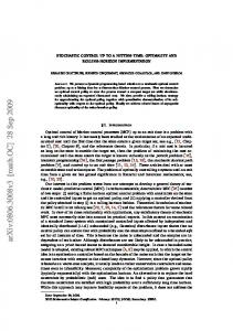
[10] where at least one instead of exactly one node from each cluster is visited. We refer to the latter version as `-GMST. Even though there are such formulations, ACSP still differs in the shape of the solution. While ACSP outputs a possibly non-simple path, `-GMST returns a tree. Moreover, it can be easily noted that a minimum spanning tree returned by `-GMST can only give a rough estimate for the size of a possibly non-simple shortest path visiting all the colors even when ACSP is required to return to the base it starts off as shown in Figure 1. When the nodes with the same color are perceived as disjoint clusters so as to interpret this figure as an instance of `-GMST, the tree spanning nodes 1 through 6 is the optimal solution to it with cost 5.
c1
2
c2
c2
c3
7 c3
3
8
is then to find the shortest possibly non-simple path that visits every distinct color at least once in this graph. The formal definition of the problem is given as: Definition 3.1. Given an undirected graph G(V, E) with a color drawn from a set C of colors assigned to each node, and a non-negative weight associated with each edge, ACSP is the problem of finding the shortest (possibly nonsimple) path starting from a designated base node s ∈ V such that every color occurs at least once on the path. The weights wi,j where (i, j) ∈ E in G correspond to distances. We will use the words weight, cost, and distance interchangeably throughout the paper. The cost of a solution to an instance of ACSP is simply the length of the path returned. ACSP can easily be shown to be NP-hard by a trivial polynomial time reduction from Hamiltonian Path (HP) problem which is well-known to be NP-complete [7]. Given an undirected graph G(V, E), HP is defined to be the problem of deciding whether it has a Hamiltonian path, namely, a simple path that visits every node in the graph exactly once.
1
c4
c4
4
9
5
c5
c5
10
c6
6
3.1. NP-hardness of ACSP Given an instance of HP, it can be transformed to the corresponding instance of ACSP as follows: Let the graph in the given HP instance be denoted by G(V, E). A new graph G0 (V ∪ {s}, E ∪ {(s, v)|v ∈ V }) is obtained by adding to G a new node s, and also the edges from s to all the original nodes in G. Next, a distinct color from C = {c1 , c2 , ..., c|V |+1 } is assigned to each and every node in G0 . The weights associated with all the edges in G0 are finally set to one. We can now state the following lemma.
11 c6
Figure 1: An example graph corresponding to an instance of ACSP. All the edges have a weight of 1, and the colors assigned to the nodes are shown next to them. Node 1 is designated as the base. The shortest path for this instance of ACSP is 1, 2, 7, 8, 9, 10, 11 which has a length of 6. When the path is constrained to return to the base, however, the path length of the solution becomes 8.
Another problem seemingly similar to ACSP is Generalized Traveling Salesman Problem (GTSP) formulated first in [12]. Given a group of possibly intersecting clusters of nodes, GTSP tries to find a shortest Hamiltonian tour with at least one (or exactly one) visit to a node from every cluster. An integer linear programming formulation for GTSP when the distance matrix is asymmetrical is given in [13]. In [14], it is shown that a given instance of GTSP can be transformed into an instance of standard TSP. In [6], GTSP is noted to be NP-hard as standard TSP is a specialization of GTSP with clusters in the form of singleton nodes. It is also surprising to note as [1] demonstrates that GTSP can be transformed into standard TSP very efficiently with the same number of nodes, but with a modified distance matrix. ACSP differs from also these variants of GTSP, in that, the nodes may be visited multiple times, and the path returned need not be a cycle.
Lemma 3.2. A given instance of HP represented with G(V, E) has a solution if and only if the corresponding instance of ACSP obtained through the lines of transformation just depicted has a solution with length |V |. Proof. Let us first prove the only if part. When the given instance of HP has a solution, there must exist a Hamiltonian path P in G given by vπ(1) vπ(2) ...vπ(i) vπ(i+1) ...vπ(|V |) of length |V |−1. As P is a Hamiltonian path, the permutation π of nodes in V is such that the edges (vπ(i) , vπ(i+1) ) ∈ E for all i ∈ {1..|V | − 1}. If we let C, and G0 (V 0 , E 0 ) denote the set of |V | + 1 colors, and the transformed graph respectively in the corresponding instance of ACSP, it is then possible to construct the path P 0 = sP in G0 with total path length |V | where s ∈ V is designated as the base node. This is apparently the shortest path visiting all distinct colors at least once. In order to prove the if part, let us assume that we have a shortest path of length |V | that starts with node s in the corresponding instance of ACSP. Since the total number of colors that needs to be visited is |V | + 1, each distinct color, and hence, the corresponding node occurs exactly once on this path. The removal of node s readily specifies a Hamiltonian path in G of the given HP instance.
3. The Problem Definition ACSP is modeled as a graph problem. The input to the problem is an undirected edge weighted graph where each vertex is assigned a color known in advance. The goal 2
The following theorem can hence be stated now.
It is shown in [10] that `-GMST, referred to as CLASS TREE problem in the paper, does not have a constantfactor polynomial time approximation algorithm (apx ) unless P = N P .
Theorem 3.3. ACSP is NP-hard. Proof. It is a direct consequence of Lemma 3.2.
Theorem 3.5. ACSP does not have a constant-factor polynomial time approximation algorithm unless P = N P .
Having learned about the NP-hardness of ACSP, a possible next step is to explore its approximability. With this objective in mind, our attention was drawn to `-GMST problem having a similar computational structure. While `-GMST looks for the minimum cost spanning tree, ACSP seeks out a possibly non-simple path with at least one node from every cluster provided that the nodes with the same color are interpreted as disjoint clusters. The following observation is first made to associate the optimal values of the respective solutions attained by both problems when fed with the same input. It is then used to report a result regarding the approximability of ACSP.
Proof. Let us assume, to the contrary, that ACSP has an apx denoted by apxACSP . Based on this assumption, an apx for `-GMST can be shown to also exist, and hence a contradiction, as follows. Given any valid input I for `-GMST, consisting of an undirected graph G(V, E) along with disjoint clusters Vi ⊆ V with 1 ≤ i ≤ k, we denote by Ij the input for ACSP obtained from I by designating j ∈ V as the base. The initial assumption with regard to the existence of an apx suggests by definition optACSP (Ij ) ≤ apxACSP (Ij ) ≤ c ∗ optACSP (Ij )
Proposition 3.4. Let I correspond to an input identified by an undirected edge weighted graph G(V, E), and a function κ : V → {1, 2, ..., k} mapping the vertices to colors. For 1 ≤ i ≤ k, Vi = {v ∈ V |κ(v) = i} induce clearly a set of k disjoint clusters, which in turn allows for a proper interpretation of I by `-GMST. Then,
for some constant c > 1, and all valid input Ij where j ∈ V . Taking the minimum over all j ∈ V , we obtain min{optACSP (Ij )} ≤ min{apxACSP (Ij )} ≤ c ∗ min{optACSP (Ij )}.
j∈V
opt`-GMST (I) ≤ min{optACSP (Ij )} < 2 ∗ opt`-GMST (I)
j∈V
j∈V
Combining this result with Proposition 3.4,
j∈V
opt`-GMST (I) ≤ min{apxACSP (Ij )} < 2∗c∗opt`-GMST (I)
holds for all valid instances I, where Ij is obtained from I by designating j ∈ V as the base node, and optA returns the cost of the optimal solution to its argument interpreted as an instance of either one of the two problems as dictated by the subscript A.
j∈V
is readily obtained. It should be noted that the minimization over apxACSP (Ij ) involves running the constantfactor approximation for ACSP separately for each j ∈ V , and the total time, even though amplified by a factor of |V |, is still polynomial in the size of a given instance. Therefore, the last inequality implies, by definition, a 2cfactor apx for `-GMST. This, however, is a contradiction, and hence, the proof.
Proof. Let us assume that the first inequality in the proposition does not hold, and, there is an instance I for which opt`-GMST (I) > minj∈V {optACSP (Ij )}. Let us suppose that s ∈ V is a node that minimizes the right-hand side of this inequality. In that case, the solution to ACSP with cost optACSP (Is ) can be easily reworked, by simply eliminating any cycles, and duplicate edges, into a tree T 0 . T 0 is clearly a solution to `-GMST for the instance I with cost less than opt`-GMST (I), and hence, contradicting the assumption. Let us assume now the latter inequality does not hold. This, for at least one instance of input I, leaves us with minj∈V {optACSP (Ij )} ≥ 2 ∗ opt`-GMST (I). Let us also assume that the tree T 0 (V 0 , E 0 ) is a solution to `-GMST with cost opt`-GMST (I) for instance I. Rooting T 0 at some s ∈ V 0 , a possibly non-simple path starting from s could be constructed visiting all the nodes in it by a depth-first search. This path, however, forms a solution to ACSP for instance Is with cost strictly less than 2 ∗ opt`-GMST (I) as no edge gets visited more than twice, and there exists at least one edge that is visited exactly once given that the return to the base is not performed upon hitting the last leaf node in V 0 . This, however, contradicts the assumption.
4. ILP Formulation of ACSP In this section, an Integer Linear Programming formulation of ACSP is presented. To this end, we start by making the following observation first. Proposition 4.1. In an optimal solution to any instance of ACSP, no edge can be visited more than once in any given direction. Proof. We assume that p is a possibly non-simple path with the shortest distance, forming a solution to a given instance of ACSP. Contrary to the proposition, we proceed by assuming that an edge (i, j) is traversed more than once in the direction from node i to node j. Highlighting the first two occurrences of this edge, then, the path can be represented as p = s, x, i, j, y, i, j, z where s is the base, and x, y, and z are sequences of zero or more nodes with edges in between consecutive nodes. It should be noted that 3
neither x nor y are allowed, by the assumption, to have any occurrences of i, and j consecutively in this order. We can, in that case, construct a new path p0 = s, x, i, y R , j, z with y R corresponding, in reverse order, to the sequence of nodes in y. This new path, p0 , visiting the same set of nodes as p, however, is shorter by 2 ∗ wi,j than p. This contradicts the optimality of p, and hence, proving the proposition.
sink. Moreover, these corresponding solutions have both the same cost. It is hence obvious that a solution to an instance of ACSP on G as given above is optimal if and only if the corresponding solution on the transformed instance employing G0 is also optimal. The ILP formulation for a given instance of ACSP can now be stated with reference to the transformation described above. X xi,j ∗ wi,j (1) minimize
Proposition 4.1 allows for an ILP formulation to ACSP where tracking down whether an edge is visited as part of an optimal solution in either one of the two possible directions becomes possible by employing a binary decision variable. This observation, coupled with the motivation to come up with a compact ILP model, form the basis of the transformation to be described next. At the heart of the transformation is the replacement of each undirected edge in a given instance of ACSP with two directed edges, and hence the adoption of a directed graph view as a substitute in the ILP formulation. Let us assume that an instance of ACSP is given, as determined by an undirected edge weighted graph G(V, E), the designated base vertex s ∈ V , and κ : V → C mapping the vertices V = {1, ..., n} to colors C = {1, ..., k}. Finally, the weights associated with the edges in G are denoted by wi,j for all unordered pairs (i, j) (or {i, j}) ∈ E. It is therefore implicitly assumed that wi,j = wj,i for all (i, j) ∈ E. In transforming G(V, E) to a directed graph G0 (V 0 , E 0 ) to be used in the ILP formulation, we first introduce two new nodes numbered 0 as the source, and n+1 as the sink, setting effectively V 0 = V ∪ {0, n + 1} in G0 . Besides, the source, and the sink are both assigned to a new color 0, extending the color set to C 0 = C ∪{0}. With the addition of the new color, κ is also augmented accordingly with κ(0) = κ(n + 1) = 0. Then, a directed edge (0, s) from the new source to the base s, as well as directed edges (i, n+1) to the sink, for all i ∈ V in G, are added into G0 with their weights set to 0. Lastly, each undirected edge (i, j) ∈ E is replaced by two directed edges (i, j) and (j, i) in G0 with both of whose weights initialized to the weight of the original edge. With this final step, the transformation sets E 0 = {(i, j), (j, i)|(i, j) ∈ E} ∪ {(0, s)} ∪ {(i, n + 1)|i ∈ V } in G0 . Continuing to use the same notation for weights in G0 , w0,s = 0, and wi,n+1 = 0 for all i ∈ V are added after the existing wi,j = wj,i for all unordered pairs (i, j) ∈ E. Any possibly non-simple path, p, starting from the designated base s, and visiting all colors at least once in G, corresponds precisely to the path 0, p, n + 1 in G0 , where nodes 0, and n+1 are the source, and the sink respectively. In the same way, a possibly non-simple path p = 0, p0 , n+1 in G0 , where p0 is a possibly non-simple path starting at s, and with length at least one, corresponds to p0 in G. As a result, the feasible solutions in G, and G0 will be in one-to-one correspondence, as long as the ILP formulation of ACSP can place a restriction on any feasible solution in G0 to start from the source, and to terminate at the
(i,j):(i,j)∈E 0
subject to x0,s = 1 X
(2) xi,j ≥ 1
, ∀c ∈ C
0
(3)
(i,j):(i,j)∈E 0 ∧ κ(j)=c
X j:(j,i)∈E 0
, ∀i ∈ V
xi,j
(4)
j:(i,j)∈E 0
, ∀(i, j) ∈ E 0
yj ≥ xi,j X i:(i,j)∈E
X
xj,i =
(5)
0
xi,j ≥ yj
, ∀j ∈ V \ {0} (6)
0
X
fj,i = yi +
j:(j,i)∈E 0
X
fi,j
, ∀i ∈ V
(7)
j:(i,j)∈E 0
xi,j ≤ fi,j ≤ (n + 1) ∗ xi,j
, ∀(i, j) ∈ E 0
(8)
0
(9)
xi,j ∈ {0, 1}
, ∀(i, j) ∈ E
yi ∈ {0, 1}
, ∀i ∈ V 0 \ {0} (10)
fi,j ∈ {0, 1, ..., n + 1}
, ∀(i, j) ∈ E 0
(11)
The objective in this formulation is to minimize the sum of the weights over all the directed edges that have been visited as shown in (1). The binary variable xi,j is set to 1 when the directed edge (i, j) is visited, and to 0 otherwise. It should be noted that all the edges involving the source, and the sink, introduced later in the transformation, with weight zero have no effect on the objective. Constraint (2) ensures that the edge from the source to the base is always a part of any feasible solution. Therefore, any feasible path always starts from the source, and then moves straight to the base. Constraint (3) demands for each distinct color that the number of the visited edges directed at the nodes with this same color is at least one. As a result, every distinct color gets visited at least once. As the constraint must also hold for color 0, any feasible path is guaranteed to terminate at the sink. Constraint (4) is used to make sure that the number of the visited edges that enter into any node i in G is equal to the number of the visited edges that leave it. This obviously holds for all the nodes, but the source, and the sink in G0 . The main ingredient in enforcing the shape of the solution to a possibly non-simple path is this constraint. Constraints (5), and (6) establish collectively the rules associated with the variables yj for all j ∈ V 0 \ {0}. The binary decision variable yj is set to 1 if and only if node j has been visited in a feasible solution. 4
Constraint (5) simply asserts that visiting an edge (i, j) is an implication of visiting node j while Constraint (6) predicates the converse. Constraint (7), along with (8), is used to eliminate any possible sub-tours, and to ensure connectedness to the base. Constraint (7) employs nonnegative integer valued flow variables, denoted by fi,j for all edges (i, j) ∈ E 0 . It enforces the total flow into a visited node to be equal to one greater than the total flow out of that node. In formulating this constraint, it is assumed that the source supplies a limited amount of flow to distribute to those nodes that are visited in any feasible solution. Hence, each node visited consumes a unit flow. Constraint (8) is in charge of regulating the flow values. A flow is associated with an edge if and only if that edge is part of a solution. As the flow is conserved at all the nodes in the original graph, the base node s is no exception. Coupled with the fact that each node visited consumes a unit flow, the edge (0, s) should carry as many unit flows as there are nodes to visit. Excluding the source leaves us with a maximum of n + 1 nodes, and hence, the factor in (8). Finally, the constraints (9), (10), and (11) are the integrality constraints for the decision variables xi,j , yi , and fi,j respectively.
Finally, a subsequent call to LP for the extended formulation is issued. Hence, the job, in this subsequent call, becomes finding the shortest possibly non-simple path that fulfills not only the previous set of constraints but also passes through every additional edge explicitly dictated by the added constraints. This process is repeated until no fractional values to process are left, and hence µ = ∅. The other two heuristics, called LPf ACSP, and LPf/x ACSP use exactly the same strategy described above except for how µ is computed before a call to LP. While LPf ACSP relies on the flow variables (µ = arg max fi,j ) in deciding which addi((i,j)∈E 0 )∧(0