map and identify locations that maximise local distance from fixed obstacles. ... adapted to grid environments, which are simpler to create than roadmaps and ...
Hierarchical Path Planning for Multi-Size Agents in Heterogeneous Environments Daniel Harabor†
Abstract— Path planning is a central topic in games and other research areas, such as robotics. Despite this, very little research addresses problems involving agents with multiple sizes and terrain traversal capabilities. In this paper we present a new planner, Hierarchical Annotated A* (HAA*), and demonstrate how a single abstract graph can be used to plan for agents with heterogeneous sizes and terrain traversal capabilities. Through theoretical analysis and experimental evaluation we show that HAA* is able to generate near-optimal solutions to a wide range of problems while maintaining an exponential reduction in effort over low-level search. HAA* is also shown to require just a fraction of the storage space needed by the original grid map.
I. I NTRODUCTION Single-agent path planning is a well known and extensively studied problem in computer science. It has many applications such as logistics, robotics, and more recently, computer games. Despite the large amount of progress that has been made in this area, to date, very little work has focused specifically on addressing planning for diverse-size agents in heterogeneous terrain environments. The problem is interesting because such diversity introduces much additional complexity when solving path planning problems. Modern real-time strategy or role-playing games (for example, EA’s popular Red Alert 3 or Relic Entertainment’s Company of Heroes) often feature a wide array of units of differing shapes and abilities that must contend with navigating across environments with complex topographical features; many terrains, different elevations etc. Thus, a route which might be valid for an infantry-solider may not be valid for a heavily armoured tank. Likewise, a car and an off-road vehicle may be similar in size and shape but the paths preferred by each one could differ greatly. Unfortunately, the majority of current path planners, including recent hierarchical planners ([1], [2], [3], [4]), only perform well under certain ideal conditions. They assume, for example, that all agents are equally capable of reaching most areas on a given map and any terrain which is not traversable by one agent is not traversable by any. Further assumptions are often made about the size of each respective agent; a path computed for one is equally valid for any other because all agents are typically of uniform size. Such assumptions limit the applicability of these techniques to solving a very narrow set of problems: homogeneous agents in a homogeneous environment. We address the opposite case and show how † Daniel Harabor and Adi Botea are affiliated with NICTA and the Australian National University, 7 London Circuit, Canberra, Australia (email: {daniel.harabor, adi.botea} at nicta.com.au).
Adi Botea† efficient solutions can be calculated in situations where both the agent’s size and terrain traversal capability are variable. First, we extend recent work on clearance-based pathfinding [4] in order to measure obstacle distance at key locations in the environment (Section IV) and show how this information helps agents plan appropriate paths (Section V). Next, we draw on a successful cluster-based abstraction technique [1] in order to produce compact yet information rich search abstractions (Section VI). Finally, we introduce HAA*, a new clearance-based hierarchical path planner (Section VIII) and provide a detailed empirical analysis of its performance on a wide range of problems involving multi-size agents in heterogeneous multi-terrain environments (Section X). II. R ELATED W ORK A very effective method for the efficient computation of path planning solutions is to make the original problem more tractable by creating and searching within a smaller approximate abstract space. Abstraction factors a search problem into many smaller problems and thus allows agents to reason about path planning strategies in terms of macro operations. This is known as hierarchical path planning. Two recent hierarchial path planners relevant to our work are described in [1] and [2], [5]. The first of these, HPA*, builds an abstract search graph by dividing the environment into square clusters connected by entrances. Planning involves inserting the low-level start and goal nodes into the abstract graph and finding the shortest path between them. The second algorithm, PRA*, builds a multi-level searchspace by abstracting cliques of nodes; the result is to narrow the search space in the original problem to a “window” of nodes along the optimal shortest-path. Both HPA* and PRA* are focused on solving planning problems for homogeneous agents in homogeneous-terrain environments and hence are not complete when either of these variables change. Our technique is similar to HPA* but we extend that work to solve a wider range of problems. In robotics, force potentials help autonomous robots find collision-free paths through an environment. The basic intution is that a robot is attracted to the far-away goal and repulsed away from obstacles as it nears them. A well known method for potential-based path planning is the Brushfire algorithm [6], which proceeds by annotating each tile on a gridmap with the distance to the nearest obstacle. This embedded information allows the robot to calculate repulsive potentials and makes it possible to plan using a gradient descent strategy. Brushfire is similar to HAA* in that the annotations it produces allow an agent to know something
about its proximity to a nearby obstacle. HAA* differs by explicitly calculating the maximal size of traversable space at each location on the map. Furthermore, unlike Brushfire, HAA* does not suffer from incompleteness which can occur when repulsive forces cancel each other out and lead the robot into a local minimum. The Corridor Map Method (CMM) [4] is a recently introduced path planner able to answer queries for multi-size agents by using a probabilistic roadmap to represent map connectivity. The roadmap (or backbone path) is comprised of nodes which are annotated with clearance information that indicates the radius of a maximally sized bounding sphere before an obstacle is encountered. Nodes are placed on the roadmap by creating Voronoi regions to split the map and identify locations that maximise local distance from fixed obstacles. Like CMM, HAA* calculates the amount of traversable space at a given location but our approach is adapted to grid environments, which are simpler to create than roadmaps and more commonly found in a range of applications. Another key difference is that we allow finegrain control over the size of the abstract graph; CMM abstractions have a fixed size. Finally, we deal with multiterrain cases making our method more information rich. Representing an environment using navigation-meshes is increasingly popular in the literature. Two recent planners in this category are Triangulation A* and Triangulation Reduction A* [3]. TA* makes use of a technique known as Delaunay triangulation to build a polygonal representation of the environment. This results in an undirected graph connected by constrained and unconstrained edges; the former being traversable and the latter not. TRA* is an extension of this approach that abstracts the triangle mesh into a structure resembling a roadmap. Like our method, both TA* and TRA* are able to answer path queries for multi-size agents. The abstraction approaches used by TA* and TRA* however are very distinctly different from our work. Where we use a simple division of the environment into square clusters, their approach aims to maximise triangle size. We also handle additional terrain requirements while both TA* and TRA* assume a homogeneous environment. III. P ROBLEM D EFINITION A gridmap is a structure composed of atomic square cells. Each grid cell is called an octile, being connected to k neighbours, where 0 ≤ k ≤ 8. Each octile is either blocked or traversable. Blocked octiles are called hard obstacles, since no agent can occupy them. Each traversable octile, t, is associated with a particular terrain type, terrain(t) ∈ T where T is the set of all possible terrains and there are r = |T | ≥ 1 possible terrains. A gridmap is representable as a graph G = (V, E) where each traversable octile generates one node v ∈ V and each octile adjacency is represented by an edge e ∈ E. An agent is any entity attempting to move across a gridmap. Every agent is square in shape and has a size s ≥ 1 : s ∈ S where S is the finite set of all agent sizes defined for a problem. An agent occupies s × s octiles,
which together correspond to its current location. Every agent has a terrain traversal capability c ⊆ T which comprises a combination of one or more terrains. Let C ⊂ 2T be the set of the capabilities c of all agents. An agent can never occupy an octile whose terrain type is not included in its capability. Thus an s × s location is traversable by an agent of size s and capability c if the terrain types of all location’s octiles are included in c. An agent can move in a cardinal direction between two s×s locations l1 and l2 if (1) both l1 and l2 are traversable by the agent and (2) the total displacement between l1 and l2 is limited to the length or width of a single octile. A diagonal move is allowed only if there exists an equivalent (but longer) two-step move using cardinal directions. A problem instance (or query) is defined as a pair of locations, start and goal, associated with an agent. A problem is valid if at least one path exists between the locations comprising only octiles traversable by the agent. IV. C OMPUTING C LEARANCE VALUE A NNOTATIONS A clearance value is a distance-to-obstacle metric associated with an octile t and a capability c. It represents the maximal length (or width) of a square whose upper-left octile is t and which contains only octiles whose terrain types are included in c. An octile can have several clearance values associated with it, one for each capability. To make our ideas easier to follow, we will use as a running example a simple environment featuring two terrain types: Ground (represented as white tiles) and Trees (represented as grey tiles). To distinguish traversable tiles from non-traversable tiles (hard obstacles) we will colour the latter in black. The set of capabilities, C, required to traverse such a map is thus defined as C = {{Ground}, {Trees}, {Ground ∨ Trees}}. We will work with agents of two sizes traversing across this environment and thus let S = {1, 2}. Figure 1 (a) to (d) illustrates how clearance can be computed with an iterative procedure in an environment as described above. In Figure 1(a) the clearance square for the highlighted traversable target tile is initialised to 1. Subsequent iterations (Figures 1(b)-(c)) extend the square and increment the clearance. The process continues until the square contains an obstacle (Figure 1(d)) or extends beyond a map boundary at which point we terminate and do not increment clearance any further. In Figure 1(e) we show the resultant clearance values for the single-terrain {Ground} capability on a toy map example (note that we omit zero-value clearances). Similarly, Figure 1(f) and Figure 1(g) show the clearance values associated with the {Trees} and {Ground ∨ Trees} capabilities respectively. Once a clearance value is derived we store it in memory and repeat the entire procedure for each capability c ∈ C. The algorithm terminates when all octiles on the gridmap have been considered. The worst-case space complexity associated with computing clearance values in this fashion is thus characterised by:
Fig. 1. (a)-(d) Computing clearance; we expand the square until a hard obstacle is encountered. (e)-(g) Clearance values for different capabilities.
Lemma 1: Let CV be the set of all clearance values required to annotate an octile gridmap with r terrains. Further, let G = (V, E) be a graph representing the gridmap where VHO ⊆ V is the set of hard obstacles. Then, |CV | = (|V | − |VHO |) × 2r−1 Proof: For a node to be traversable for some capability, the capability must include the node’s terrain type. There are 2r combinations of terrains (and hence capabilities) but a fixed terrain type will appear at most in 2r−1 capabilities. There are |V | nodes in total to represent the environment, and we avoid storing any clearance values for all nodes in VHO . The result from Lemma 1 is an upper bound; if no agent has a given capability c there is no need to store the corresponding clearances. Despite this observation, the associated exponential growth function suggests that it is impractical to store every clearance value as there are Θ(2r ) per node. Fortunately, clearance values can be computed ondemand with little effort. In particular, calculating clearance for any agent a of size s ∈ S only requires building a clearance square of maximum area s2 octiles. We present such an approach in Algorithm 1. Algorithm 1 Calculate Octile Clearance Value Require: t ∈ gridmap and c ∈ C and s ∈ S square ← t cv ← 0 while traversable(square, c) ∧ area(square) ≤ s2 do cv ← cv + 1 square ← expand(square) return cv The key advantage of calculating clearance is that we are able to map our extended problem into a classical problem, called the canonical problem, with only two types of tiles (traversable and blocked) and only atomic-size agents. We formalise this as: Theorem 2: Given an annotated gridmap and an agent of arbitrary size and capability, any path planning problem can be reduced to a classical path planning problem, where the size of the agent is one octile and the capability of the agent is one terrain. Proof: Consider an agent a of size sa and capability ca . Consider further a location l of size sa × sa , its upper-left
octile ul, and the clearance value cv(ul, ca ) associated with the octile ul and the capability ca . It is easy to observe that the location l is traversable by the agent a if and only if cv(ul, ca ) ≥ sa . This allows us to map the original problem into a classical path planning problem as follows: The agent a, which currently occupies an sa × sa location l, is mapped into an atomic-size agent whose location is ul. When searching for a path, any octile t is traversable by the atomic-size agent only if cv(t, ca ) ≥ sa . All other octiles are regarded as blocked. This is a useful result because it indicates that we can apply abstraction techniques from classical path planning to answer much more complex queries involving a wide range of terrain type and agent-size variables. In particular, if topological abstraction that partitions a gridmap into disjoint clusters were applied directly to a problem with arbitrary-size agents, a large agent could be in several clusters at a time. This raises a number of challenges which we found difficult to handle. The theorem above elegantly eliminates this problem, since an atomic-size agent can be in only one cluster at a time. V. A NNOTATED A* Low-level planning for our extended problem using clearance values is a straightforward application of the ideas thus far. To compute an optimal shortest path between a start and goal node we use a variation on the classical A* algorithm [7], which we term Annotated A* (AA* for short). Our approach differs from standard A* by requiring two additional parameters for each query: the agent’s size and capability. Recall that clearance can be computed on demand for each visited location. Therefore, each atomic octile under consideration by the algorithm can be dynamically evaluated as either blocked or traversable. This allows us to map any query into a canonical problem as shown earlier. VI. C LUSTER - BASED M AP A BSTRACTION AA* is sufficient for low-level planning on the original gridmap but inefficient for large problem sizes; we would prefer to express a better strategy using macro-operators. Existing hierarchical path planning approaches, particularly those focused on gridmaps such as [1] and [2], achieve this by decomposing the gridmap into discretised adjacent areas. Each pair of neighbouring areas are connected by a single shortest path and each canonical problem is mapped into this much smaller hierarchical representation. When we introduce agents of arbitary sizes and capabilities however previous abstraction techniques break down because they produce incomplete hierarchical abstractions. In particular, there may be several shortest paths between each pair of adjacent areas, potentially one for each combination of agent size and capability. To solve this problem we build on our result from theorem 2, which is key to the spatial abstraction described in this section. Our technique extends the process in [1], which involves dividing a grid map into fixed-size square sections called clusters. Figure 2(a) shows the result of this decomposition
approach; we use clusters of size 5 to split our toy map into 4 adjacent clusters. In the original work, entrances are defined as obstaclefree transition areas of maximal size that exist along the border between two adjacent clusters. Each entrance has one or two transition points (depending on its size), which are represented in an abstract search graph by a pair of nodes connected with an undirected inter-edge of weight 1.0. We use a similar approach but require as a parameter C, the set of all capabilities, and thus attempt to identify entrances for each c ∈ C.
Fig. 2. (a) Decomposing the grid map into 5 × 5 clusters. (b) 3 entrances are identified between clusters C1 and C3. (c) Transition points between clusters C1 and C3.
Given a capability c, we start at the first pair of traversable tiles (i.e., tiles whose terrain type is in c) along the adjacent border area and extend each entrance until one of three termination conditions occurs: the end of the border area is reached, an obstacle (i.e., either a hard obstacle or a traversable tile whose terrain type is not in c) is detected, or the clearance value of nodes along the border area in either cluster begins to increase. The last condition is important to preserve representational completeness for large agents in cases where a cluster is partially divided by an obstacle (such as a wall) near the border. By leveraging clearance we are able to reason about the presence of such obstacles and build a new entrance each time we detect the amount of traversable space inside either cluster is increasing. Once an entrance is found, we choose as the transition point the first pair of adjacent nodes in each cluster which maximise clearance for c. The clearance of a pair of adjacent nodes (n1 , n2 ) for a given capability c is defined as cv(n1 , n2 , c) = min(cv(n1 , c), cv(n2 , c)). Thus, we add to the abstract graph a new edge between the two nodes, einter , and annotate it with the corresponding capability and clearance value. The algorithm repeats for each c ∈ C and terminates when all adjacent clusters have been considered. This ensures we identify all possible entrances for each available capability. In Figure 2(b) we present three entrances identified by scanning the border between clusters C1 and C3. Entrances E1 and E2, each of which span only part of the border area, are discovered using the {Ground} and {Trees} capabilities respectively. E3, which spans the whole border area, is discovered using the {Ground ∨ Trees} capability. The connected tiles represent the locations of the subsequent
transition points; the final result is shown in Figure 2(c). Note that E1 and E3 are incident on the same pair of nodes in the abstract graph. This is due to our strategy of attempting to re-use any existing nodes from the abstract graph. The final step in the decomposition involves attempting to add to the abstract graph a set of intra-edges for each pair of abstract nodes inside a cluster. We achieve this by running multiple AA* searches ∀(c, s) : c ∈ C, s ∈ S. Once a path is found we annotate the new edge, eintra , with the capability and clearance parameters used by AA* and set its weight equal to the cost of the path. The algorithm terminates when all clusters have been considered. We thus construct an abstract multi-graph in which each edge e is annotated with a capability ce and a clearance value cv(e, ce ). Each e ∈ Eabs is traversable by an agent a of size sa and capability ca iff ce ⊆ ca ∧cv(e, ce ) ≥ sa . We term the resultant abstraction initial and give the following lemmas to characterise its space complexity: Lemma 3: Let Vabs represent the set of nodes in an abstract graph of a gridmap which is perfectly divisible into c × c clusters, each of size n × n. Then, in the worst case, the total number of nodes is given by: |Vabs | = 4(2n − 1) + (4c − 8)(3n − 2) + (c − 2)2 (4n − 4) Proof: Each transition point results in two nodes in the abstract graph. If there are no hard obstacles and every pair of nodes along the adjacent border between two clusters has different terrain type then there will be a maximal number of transition points. In this scenario, clusters in the middle of the map, of which there are (c − 2)2 , have 4 neighbours and each one contains 4n − 4 nodes. Clusters on the perimeter of the map (excluding corners), of which there are 4c − 8, have 3 neighbours and 3n − 2 nodes. Corner clusters, of which there are 4, have 2 neighbours and each contains 2n − 1 nodes. Lemma 4: Let Eabs (L) ⊂ Eabs represent the set of intraedges for a cluster L that contains x abstract nodes. Further, let r be the total number of terrains found in the map and k the number of distinct terrain types found inside L. Then, the number of intra-edges required to connect all nodes in L is, in the worst case: x(x − 1) 2 Proof: For each pair of abstract nodes in a cluster and each size/capability combination, we compute at most one path of optimal length. From Lemma 1 we know each node is traversable at most by 2r−1 capabilities thus there must be at most |S| × 2r−1 ways of covering 2 nodes. However, the number of terrains inside a cluster is governed by its size; only k ≤ r terrains may be found. From this, it follows that the upper-bound on the size of the set of edges covering each pair of nodes is in fact |S| × 2k−1 . In the worst case, there will be a maximal number of edges between each pair of such pairs in total per cluster. nodes and there are x(x−1) 2 |Eabs (L)| = |S| × 2k−1 ×
Lemma 5: Let Einter ⊂ Eabs represent the set of interedges in an abstract graph of a grid map. In the worst case, the map is perfectly divisible into c × c clusters, each of size n × n and the number of inter-edges is given by: n(n − 1) |Einter | = (2c2 − 2c) × 2 Proof: We know from the proof of Lemma 3 that in the worst case each tile along the border between two adjacent clusters is represented by a node in the abstract graph. If we count the number of adjacencies, avoiding duplication, we find there are 2c2 − 2c in total. Each transition results in an inter-edge and there are n single-terrain transitions with clearance 1 per adjacency and some number of inter-edges to represent multi-terrain transitions with larger clearances. By observation we can see that that each adjacency will produce [n single-terrain transitions]...[1 n-terrain transition]. This recurrence relation holds for the general sequence counting formula n(n−1) 2 The above results are interesting for several reasons. Firstly, Lemma 3 shows that the number of nodes in the graph is a function of cluster-size. This suggests that by varying the dimensions of clusters we can trade a little performance (the time it takes to traverse a cluster) for memory (less abstraction overhead). The results in Lemma 4 and 5 seem to support this hypothesis. We see that the number of edges between nodes in the graph is mostly dependent on the complexity of the clusters in which they reside rather than exponential in the number of capabilities. This is important because it means that, despite having an exponential abstract edge growth function, we can directly control the size of the exponent. The cluster-based decomposition technique allows us to include as much or as little complexity in each cluster as we require. VII. O PTIMISING A BSTRACT G RAPH S IZE As we have observed in lemmas 4 and 5, the initial abstraction algorithm attempts to represent every optimal path between clusters and inside clusters. However, most maps have far simpler topographies than the worst-case; in our experimental scenarios we often observed the same path returned for different pairs of (c, s) parameters when discovering intra-edges. This presents us with an opportunity to compact the graph by removing unnecessary duplication from the abstract edge set. Consider the initial abstraction in Figure 3(a) and contrast it with our desired result in Figure 3(b). {E3, E5} represent the same path between nodes w and y but are annotated with different clearance values. The same is true for {E4, E6} which both cover nodes u and y. In such cases we say that E3 and E4 are strongly dominant, which we denote E3 ≻ E5 and E4 ≻ E6. This is an irreflexive and asymmetrical relationship between edges which we formalise as: Theorem 6: Let {ea , eb } ∈ Eabs be two distinct edges which connect the same pair of abstract nodes and are
annotated with capabilities ca ⊆ cb such that: cv(ea , ca ) ≥ cv(eb , cb ) ∧ weight(ea ) = weight(eb ) Then ea ≻ eb and we may remove eb from Eabs without loss of generality or optimality. Proof: Since ca ⊆ cb , it must be the case that any agent with the correct capability to traverse eb must be likewise able to traverse ea . Further, if cv(ea , ca ) ≥ cv(eb , cb ) holds, it must also be the case that any agent large enough to traverse eb is also large enough to traverse ea . These conditions are sufficient to preserve generality. Finally, since ea is equal in weight to eb , we cannot lose optimality by removing eb . We term the resultant graph in which all strongly dominant edges have been removed a high-quality abstraction.
Fig. 3. (a) A cluster in an initial abstraction. (b) The same cluster once strong edge dominance is applied.
A further observation made during our analysis of this problem was that in many cases there exist multiple alternative routes to reach a goal location. The shortest paths tended to involve the traversal of optimal-length multi-terrain edges. However, it was often possible to reach the same destination using slightly longer single-terrain edges. This suggests that the abstract graph can be further compacted without affecting the completeness of the representation. In Figure 4(a) and 4(b) we show a typical high quality abstraction while in Figure 4(c) and 4(d) we highlight the desired result after further compacting the graph. In this
Fig. 4. (a) A high quality abstraction of our toy map; note that some edges overlap and are not uniquely visible. (b) Inter-edges associated with the high quality graph. (c) The resultant graph after applying weak dominance. (d) Inter-edges associated with the low-quality graph.
example we can see that, although edges E1 and E2 have different traversal requirements, any agent of size s ∈ {1, 2} capable of traversing E2 can also traverse E1 without loss of generality. In such cases we say E1 is weakly dominant and denote it as E1 % E2. Notice also that E3 % E4, E6 % E7, E10 % E8 and E10 % E9. Unlike the case of strong dominance, only representational completeness (and not optimality) is retained. We formalise it as:
does affect the quality of computed solutions. In the worst case, a one-step transition of cost 1.0 in a high quality graph may be as long as f (n) = 4n + f (n − 2) : f (2) = 3, f (3) = 13, where n ≥ 2 is the length of a n × n cluster. This is a pathological case however; as we will show the differences in real-world scenarios are much smaller and still near-optimal. The choice of which quality abstraction technique to employ will depend on the requirements of the specific application; it is a classic tradeoff between run-time performance vs space.
Theorem 7: Let La and Lb be two adjacent clusters, and {wa , xb }, {ya , zb } ∈ Vabs two pairs of abstract nodes, each pair connecting La and Lb . Denote the inter-edges associated with these node pairs as {ewx , eyz } ∈ Eabs and suppose they are annotated with clearance values cv(ewx , cwx ), cv(eyz , cyz ) : cwx ⊆ cyz ∈ C. In this scenario, ewx % eyz iff the following conditions are met: 1) The clearance dominance condition: cv(ewx , cwx ) ≥ cv(eyz , cyz ). 2) The circuit condition: ∃ewy , exz ∈ Eabs , annotated with the capabilities cwy ⊆ cyz and cxz ⊆ cyz , which connect {wa , ya } and {xb , zb } such that cv(ewy , cwy ) ≥ cv(eyz , cyz ) and cv(exz , cxz ) ≥ cv(eyz , cyz ). Then, any location which can be reached by traversing eyz can also be reached via ewx .
VIII. H IERARCHICAL P LANNING
Proof: If a circuit exists between the set of edges {ewx , eyz , ewy , exz } in which every edge is traversable by cyz with a clearance value at least equal to cv(eyz , cyz ), then it follows that any nodes in La or Lb which are reachable from ya or zb must be reachable from wa or xb . Thus, any destination an agent can reach via eyz can also be reached via ewx . Corollary 8: If ewx % eyz , then ya and zb and are also dominated and can be removed, unless required by another (non-dominated) inter-edge. Proof: If ya and zb are required by a non-dominated inter-edge, we cannot remove them without violating the clearance dominance condition which is required to retain representational completeness. If this is not the case however, we know by the circuit condition that any node reachable by an intra-edge via ya or zb is also reachable via the endpoints of ewx . Thus, both nodes and any associated intra-edges dependent on them can be safely removed. In many situations, multi-terrain inter-edges tend to be associated with very large clearances; much larger than the size of our largest agent. This unnecessarily limits the applicability of the clearance dominance condition from Theorem 7. Leveraging the fact that sM = maxs∈S s is known, we can maximise the number of edges which are weakly dominated by applying the following truncation condition to Eabs before Theorem 7: ∀e ∈ Eabs (cv(e, ce ) > sM ⇒ cv(e, ce ) ← sM ) Of course, opting for a low-quality abstraction in this way
Given a suitable graph abstraction, we can once more turn our attention back to agent planning. In order to compute a hierarchical solution to a canonical problem, we employ a similar process to that described in [1]. We provide a brief overview of their method here; for a more detailed description, we direct the reader to the original work. We begin by using the x, y coordinates of the start and goal nodes to identify the local cluster each is located in. Next, we insert two temporary nodes into the abstract graph (which we remove when finished) to represent the start and goal. Connecting the nodes to the rest of the graph involves attempting to find an intra-edge from each node to every other abstract node in the cluster using AA*. This phase involves i + j searches in total, corresponding to the number of combined abstract nodes in the start and goal clusters. To compute a high-level plan we again use a variation on A* – this time to evaluate the annotations of abstract edges before adding a node to the open list. Once the search terminates we can take the result, and, if immediate execution is not necessary, we are finished. Otherwise, we refine the plan by performing a number of small searches in the original gridmap between each pair of nodes along the abstract optimal path. We term this algorithm Hierarchical Annotated A* (HAA* for short). IX. E XPERIMENTAL S ETUP We evaluated the performance of AA* and HAA* on a set of 120 octile-based maps, ranging in size from 50x50 to 320x320, which we borrowed from a popular roleplaying game. The same maps were used in previous games-related research (e.g., [1]). In their default configuration, the maps only featured one type of traversable terrain interspersed with hard obstacles. We therefore created five derivative sets (making for a total of 720 maps) where each traversable tile on every map had one of {10%, 20%, 30%, 40%, 50%} probability of being converted into a second type of traversable terrain. Octiles with this terrain type are called soft obstacles, as they are not traversable by all agents. This allowed us to evaluate the algorithms in environments with both soft and hard obstacles. For each map we generated 100 experiments by randomly creating valid problems between arbitrarily chosen pairs of locations and some random capability. We used two agent sizes in each experiment: small (occupying one tile) and large (occupying four tiles) resulting in 144,000 problem instances (720x200) overall. All experiments were conducted on a
CS15 LQ CS20 HQ
30% SO
40% SO
50% SO
16.6%
17.7%
18.3%
18.5%
Edges
8.2%
32.6%
38.4%
37.8%
35.7%
35.0%
Nodes
5.3%
7.9%
10.3%
12.8%
15.0%
15.7%
Edges
2.2%
6.7%
Nodes
5.6%
9.6%
Edges
6.0%
28.0%
Nodes
2.9%
4.8%
Edges
1.2%
Nodes
11.6%
17.0%
22.0%
23.6%
11.0%
11.8%
12.2%
12.3%
32.4%
32.1%
30.0%
29.4%
6.4%
8.1%
9.7%
10.3%
4.6%
8.5%
12.5%
17.2%
18.8%
4.0%
7.0%
8.1%
8.8%
9.1%
9.2%
Edges
5.0%
25.0%
28.8%
28.3%
26.3%
26.0%
Nodes
2.0%
3.4%
4.6%
5.9%
7.2%
7.6%
Edges
0.9%
3.6%
6.9%
10.1%
14.4%
15.8%
(a) Path Quality vs. Soft Obstacles ●
(b) Path Quality vs. Agent Size (CS15) 15
20% SO
14.6%
CS10 HQ CS10 LQ CS15 HQ CS15 LQ CS20 HQ CS20 LQ
●
●
●
● ●
●
● ●
●
0
The first thing to notice is that in all cases the abstract graph is only a fraction the size of the original graph. As expected, larger clusters generate smaller graphs; the smallest abstractions are observed on the SO 0% problem set using CS20. In this case, using a HQ abstraction results in 4.0% the number of nodes found in the original graph and 5.0% edges. LQ abstractions are even better featuring just 2.0% as many nodes and 0.9% edges. The total space complexity associated with storing a graph is given by the total amount of space required to store both nodes and edges. If we assume each non-abstract node and edge require one byte of memory to store, then our smallest abstract graph, which contains 2 annotations per edge (capability and clearance, together requiring 1 additional byte), will have a space complexity 8.7% the size of the original graph using a HQ abstraction and just 1.8% using an LQ abstraction. Similarly, the largest HQ graph, which occurs for CS10 on SO 20%, has a space complexity 63.8% the size of the original. By comparison, LQ graphs are largest for CS10 on SO 50%; here 40.4% the size of the original gridmap. Moving from CS10 to CS20 reduces the worst-case space complexity of HQ graphs to 47.0% and 26.4% for LQ graphs. Interestingly, if we use the number of nodes as an indicator for the number of inter-edges in a graph, we may deduce that most HQ graphs are predominately composed of intra-edges. The exact number depends on the density of soft obstacles in clusters; less dense clusters (as found on SO 20%) result in
●
●
●
30
40
50
0
0
●
CS20 LQ
Size=1 HQ Size=1 LQ Size=2 HQ Size=2 LQ
10
CS15 HQ
10% SO
9.0%
% error
CS10 LQ
0% SO Nodes
5
CS10 HQ
15
TABLE I S IZE OF ABSTRACT GRAPH WITH RESPECT TO ORIGINAL GRAPH .
apl − opl × 100 opl where opl is the length of the optimal path as calculated by AA* and apl the length of the abstract path used by HAA*. %error =
10
In Table I we present the size of the abstract graphs relative to the size of the original graphs which featured an average 4469 nodes and 16420 edges. We look at the effect of increasing the amount of soft obstacles (SO) from 0% (the original test maps with only one traversable terrain) to 50%. We also contrast high and low quality abstractions (denoted HQ and LQ) on a range of cluster sizes {10, 15, 20} (denoted CS10, CS15 and CS20).
% error
X. R ESULTS
more intra-edges as more unique paths (of differing sizes and capabilities) are found between each pair of abstract nodes. This is consistent with Lemma 4 and useful to understanding the worst-case behaviour of HQ abstractions. The linear increase in the size of LQ graphs is the result of a greater number of single-terrain entrances found as the number of soft obstacles increases (an observation consistent with Lemma 3). Increasing the density of soft obstacles in a cluster causes the circuit condition from Theorem 7 to be less often satisfied and leads to the observed worst-case on SO 50%. Next we consider the performance of HAA* with respect to path quality. We measure this as:
5
2.4GHz Intel Core 2 Duo processor with 2GB RAM running OSX 10.5.2. To implement both planners we used the University of Alberta’s freely available pathfinding library, HOG (www.cs.ualberta.ca/˜nathanst/hog.html).
10
20
30
% soft obstacles
Fig. 5.
40
50
0
10
20
% soft obstacles
HAA* performance (HQ vs LQ abstraction)
Figure 5(a) shows the average performance of HAA* with respect to cluster size and soft obstacles. Notice that HQ graphs yield a very low error; in most cases between 3-6%. Perhaps most encouraging however are the results for LQ abstractions, where in most cases HAA* performs within 610% of optimal. The highest observed error in both cases occurs on SO 0% and is due to our inter-edge placement strategy. In all situations the pair of nodes with maximal clearance in an entrance, which we choose as our transition point, tends to be towards the beginning of the entrance area which is not an optimal placement. On maps that produce low-complexity clusters of predominantly one terrain, this results in long entrances that are poorly represented by a single inter-edge. Increasing the amount of soft obstacles produces shorter entrances and generates more transition points, leading to a significant reduction in error. It appears HAA* is so optimised for complex cases that it suffers some minor performance degradation on simpler problems. Interestingly, the error associated with both HQ and LQ abstractions reaches a minimum on SO 20% before gradually increasing toward SO 50%. To better understand this phenomenon we present in Figure 5(b) the performance of both small and large agents on HQ and LQ graphs using a fixed cluster-size of 15. Notice that the performance of small agents continues to improve beyond SO 20% while
large agents begin to degrade. The observed rise in error stems from the decreasing size of entrances on the problem sets featuring denser clusters. As previously shown in Table I, maps with more soft obstacles result in a greater number of smaller single-terrain entrances. This situation is beneficial for small-size agents (there are more transitions to choose from) but is disadvantageous for large-size agents who must more and more often traverse from one cluster to another via a single transition point: the one which results from a long multi-terrain entrance that spans the length of the border area between two clusters. Each such traversal is usually suboptimal and degrades the quality of the path. The worst case is observed on the SO 50% dataset where the performance of HAA* begins to approach that seen on the SO 0% dataset.
15000
(b) Total search effort (SO 20%, LQ)
●
●
●
●
● ●
avg. nodes expanded
10000
●
AA* HAA* CS10 HAA* CS15 HAA* CS20
●
●
●
10000
●
●
●
●
●
● ●
●
●
●
●
●
●
●
●
0
●
●
●
●
0
0
● ●
100
●
●
5000
AA* HAA* CS10 HAA* CS15 HAA* CS20
5000
avg. nodes expanded
15000
(a) Total search effort (SO 20%, HQ) ●
200
300
optimal solution length
Fig. 6.
400
●
0
●
●
●
100
200
300
400
optimal solution length
HAA* total search effort (nodes expanded).
Finally, we turn our attention to Figure 6, where we evaluate HAA* using a search effort metric. Here we contrast the total number of nodes expanded by HAA* (during insertion, hierarchical search and refinement phases) with AA* on both HQ and LQ graphs. We focus on the SO 20% problem set in order to analyse the effect on search effort as path length increases but note that similar trends hold for the other problem sets. Looking at Figure 6(a) we observe that agents using HQ graphs featuring large cluster-sizes are disadvantaged in this test. The insertion effort required to connect start and goal to each abstract node in their local clusters heavily dominates the total effort causing HAA* CS20 to trail AA* for problems up to length 250. We can see the gap between CS20 and the smaller cluster sizes decrease as the problem size grows. By comparison, in Figure 6(b) we see that the difference is less pronounced using LQ graphs (there are less abstract nodes per cluster). However, it appears CS10 or CS15 are more suitable choices for problems up to our maximum length, 450. The average time required to compute a solution was observed to have very similar trends to those shown in Figure 6; on this particular dataset HAA* averaged 6.3ms and 3.7ms per query using HQ and LQ graphs respectively. This further reiterates the applicability of our technique to real-world applications such as games, where computational resources available for path planning are highly constrained.
XI. C ONCLUSION Heterogeneity in path planning is characteristic of many real-world problems but has received very little attention to date. In this paper we have addressed this issue by showing how clearance-based obstacle distances can be computed and leveraged to improve path planning for multi-size agents in heterogeneous-terrain grid-world environments. Our approach reduces complex problems involving agents of different sizes and multi-terrain traversal capabilities to much simpler single-size, single-terrain search problems. Building on these new insights, we have introduced a new planner, Hierarchical Annotated A*, and have shown through comparative analysis that HAA* is able to find near-optimal solutions to problems in a wide range of environments yet still maintain exponentially lower search effort over standard A*. Our hierarchical abstraction technique is simple to apply but very effective; we have shown that in most cases the overhead for storing the abstract graph is a small fraction of that associated with non-abstract graphs. Future work could involve looking at computing annotations to deal with elevation and other common terrain features. We are also interested in finding a better inter-edge placement approach and reducing the effort to insert the start and goal into the abstract graph. Finally, we believe HAA* could be usefully applied to solving heterogeneous multiagent problems. XII. ACKNOWLEDGEMENTS We thank Philip Kilby and Eric McCreath for their help and insightful comments during the development of this work. NICTA is funded by the Australian Government as represented by the Department of Broadband, Communications and the Digital Economy and the Australian Research Council through the ICT Centre of Excellence program. R EFERENCES [1] A. Botea, M. M¨uller, and J. Schaeffer, “Near optimal hierarchical pathfinding,” Journal of Game Development, vol. 1, no. 1, pp. 7–28, 2004. [2] N. R. Sturtevant and M. Buro, “Partial pathfinding using map abstraction and refinement,” in AAAI, 2005, pp. 1392–1397. [3] D. Demyen and M. Buro, “Efficient triangulation-based pathfinding,” in AAAI, 2006, pp. 942–947. [4] R. Geraerts and M. Overmars, “The corridor map method: a general framework for real-time high-quality path planning,” Computer Animation and Virtual Worlds, pp. 107–119, 2007. [5] V. Bulitko, N. R. Sturtevant, J. Lu, and T. Yau, “Graph abstraction in real-time heuristic search,” J. Artif. Intell. Res. (JAIR), vol. 30, pp. 51–100, 2007. [6] J. Latombe, Robot Motion Planning. Kluwer Academic Publishers, 1991. [7] P. E. Hart, N. J. Nilsson, and B. Raphael, “A formal basis for the heuristic determination of minimum cost paths,” IEEE Transactions on Systems Science and Cybernetics, no. 4, pp. 100–107, 1968.