AbstractâThe stability of networked control systems (NCS) can be analyzed using jump systems where the jumping charac- terizes packet loss or delay.
Proceedings of the 46th IEEE Conference on Decision and Control New Orleans, LA, USA, Dec. 12-14, 2007
ThB02.4
Almost Sure Stability and Transient Behavior of Stochastic Nonlinear Jump Systems Motivated by Networked Control Systems Rainer Blind, Ulrich M¨unz, Frank Allg¨ower Abstract— The stability of networked control systems (NCS) can be analyzed using jump systems where the jumping characterizes packet loss or delay. This motivates our investigations on nonlinear jump systems (NLJS). In many cases, the transient behavior of such a system, i.e. the convergence rate to the equilibrium, is much more interesting than the mere stability. In this paper, we extend a recent result that describes this transient behavior for NCS with packet loss to NCS with random delays. In other words, the jump system exhibits an arbitrary but finite number of discrete states instead of only two states. In addition, we considerably reduce the conservatism of the former result, which is shown theoretically and through a simple numerical example. Index Terms— Nonlinear jump systems, almost sure stability, transient behavior, networked control systems, stochastic delays.
I. I NTRODUCTION The control of dynamical systems via digital networks has attracted an increasing attention over the last years, see e.g. the special issues [1]–[3]. This research is mainly driven by applications like distant operation and diagnosis or sensors and actuators connected to the controller via communication networks. If we assume that there is a constant stream of data over the digital communication channel, then we have to consider two different network properties: packet dropout and packet delay. A common approach to model the loss and delay of packets in networked control systems (NCS) is the construction of a jump linear system (JLS). The stability of this JLS is then studied in order to derive the stability of the NCS, see [4]–[7]. Most of these publications on JLS deal with second moment (s.m.) or almost sure (a.s.) stability. Their definition and a comparison can be found in [8]. Although stability conditions for JLSs are well-known, see [8]–[11], less is known about their transient behavior. In [8], it is stated that |x| decreases approximately exponentially if the system is a.s. stable. However, it is still possible that |x| exceeds any bound if one or more of the subsystems are unstable. Even if the system is s.m. stable, which is more conservative than a.s. stability [8], we cannot guarantee that an arbitrarily large bound is never exceeded. We can circumvent this problem and also get a precise description for the transient behavior if we determine a bound that is only exceeded with a very small probability. It would be even better if this bound decays exponentially to the equilibrium. This has been studied in [4] R. Blind, U. M¨unz, and F. Allg¨ower are with the Institute for Systems Theory and Automatic Control, University of Stuttgart, Stuttgart, Germany. {blind, muenz, allgower}@ist.uni-stuttgart.de. U. M¨unz’s work was financially supported by The MathWorks.
1-4244-1498-9/07/$25.00 ©2007 IEEE.
for nonlinear jump systems (NLJS) with two subsystems. This work was motivated by NCS with packet dropout. In this paper, we expand this idea for a general class of NLJS with independent and identically distributed (iid) jumping between a finite set of possible subsystems. This is motivated by NCS with random delay and packet dropout. Apart from the generalization to a jump system with an arbitrary number of subsystems, we considerably reduce the upper bound given in [4]. This is shown theoretically and through a simple numerical example in this paper. The paper is organized as follows: The problem statement as well as some preliminary results are presented in Section II. The a.s. stability is studied in Section III. In Section IV, we present our main result, the new upper bound of the confidence limit. A simple example is studied in Section V before the paper is concluded in Section VI. Notation: We call a function φ : R≥0 → R≥0 of class K if it is continuous, zero at zero, and strictly increasing. We say φ ∈ K∞ if it is additionally unbounded. A function ϕ : R≥0 → R≥0 is said to be of class L if it is continuous, nonincreasing, and limt→∞ ϕ(t) = 0. Moreover, we call a function Φ : R≥0 × R≥0 → R≥0 of class KL if it is of class K in the first argument and of class L in the second argument (cf. [4]). Finally, the set of natural numbers N does not contain zero. We write Z+ to address all nonnegative integers including zero. II. P ROBLEM S TATEMENT AND P RELIMINARIES A. Problem Statement We consider systems that consists of d discrete-time subsystems x(k + 1) = fi (x(k)), i ∈ N = {1, 2, . . . , d}, where the jumping is driven by a random process {r} : Z+ → N : x(k + 1) = fr(k) (x(k)) , x(0) = x0 6= 0 ,
(1)
with state x ∈ Rn and initial condition x0 . The subsystems are driven by nonlinear functions fi . We assume that the origin is an equilibrium for all subsystems, i.e. fi (0) = 0, ∀i ∈ N . This model is an extension of the NLJS in [4]. Our analysis of systems of class (1) is motivated by investigating the behavior of NCS of the form x ˜(k + 1) = A˜ x(k) + B u ˜(k) u ˜(k) = κ(k)K x ˜(k − τ (k))
(2) (3)
where the random processes {κ} : Z+ → {0, 1} and {τ } : Z+ → N = {0, 1, . . . , τ¯} model the stochastic packet dropout and delay, respectively. We assume that packets with
3327
46th IEEE CDC, New Orleans, USA, Dec. 12-14, 2007 a delay larger than τ¯ are dropped. We augment the state x ˜(k) with all delayed states x ˜(k − τi ), τi ∈ N \ {0} and get the linear jump system x(k + 1) = A(κ(k), τ (k))x(k),
(4) T
where x(k) = [˜ x(k), x ˜(k − 1), . . . , x ˜(k − τ¯)] and A depends on A, B, and K as well as κ and τ . Clearly, system (4) is a special case of (1) with d = τ¯ +2. d−1 subsystems fi correspond to the fixed delays τi ∈ N . A further subsystem represents the open-loop system caused by packet losses. Even though our work is motivated by NCSs of class (4), all results are derived and valid for the general class of NLJSs (1). Before this results are derived, we give the assumptions that are used in the theorems: Assumption 1: There exist functions δ1 , δ2 ∈ K∞ , a Lyapunov candidate V : Rn → R≥0 , and constants 0 < λmin ≤ λi ≤ λmax such that for all x ∈ Rn δ1 (|x|) ≤ V (x) ≤ δ2 (|x|)
(5)
and V (fi (x)) ≤ λi V (x) ,
∀i∈N.
(6)
Note that λmax < 1 is not assumed, i.e. some subsystems may be unstable. Without loss of generality, we further assume that λi are sorted such that λmin = λ1 ≤ λ2 ≤ · · · ≤ λd = λmax .
(7)
For further studies, we define the ith discrete state indicator function αi (k) as ( 1 if r(k) = i αi (k) := (8) 0 else and assume that its expectation value α ¯ i > 0 does not depend on the time k: © ª α ¯ i := E[αi (k)] = Pr r(k) = i . (9)
Assumption 2: The random process {r} is a sequence of independent identically distributed (iid) random variables, i.e. © ª Pr r(k) = i | r(l) = j = α ¯ i , ∀i, j ∈ N, 0 ≤ l < k , © ª © ª Pr r(k) = i = Pr r(l) = i = α ¯ i , ∀k, l ∈ Z+ .
Assumption 3: The random processes {αi } are mean ergodic, i.e. ( ) k−1 1X (10) αi (j) = α ¯ i = 1, ∀ i ∈ N. Pr lim k→∞ k j=0 Note that the strong law of large numbers states that Assumption 2 implies Assumption 3, (see e.g. [12], Section III.7, Theorem 2). B. Hoeffding’s Inequality We use Hoeffding’s Inequality to prove our main result in Theorem 5. This inequality gives an upper bound for
ThB02.4 the probability that the sum S of m independent random variables exceeds its mean E[S] by a positive number mt. Lemma 1 (Hoeffding’s Inequality, [13]): If X1 , X2 , · · · , Xm are independent random variables with finite first and second moments, S = X1 + · · · + Xm and a ≤ Xi ≤ b for i = 1, . . . , m, then for t > 0 © ª 2 2 Pr S − E[S] ≥ mt ≤ e−2mt /(b−a) . (11) There are alternatives for the right-hand side of (11) that could lead to less conservative results in some cases (cf. [13]). III. A LMOST S URE S TABILITY In this section, we give an a.s. stability condition for (1). The a.s. stability of (1) is defined as follows: Definition 1 (a.s. stability): The NLJS (1) is a.s. stable if almost all solutions of (1) converge to the origin as k → ∞, i.e. ½ ¾ Pr lim |x(k)| = 0 = 1. (12) k→∞
For the stability analysis based on the Lyapunov candidate V , the jumping of the subsystems fi can be interpreted as jumping of the Lyapunov coefficients λi . Hence, we get ¡ ¢ V (x(k)) = V fr(k−1) (x(k − 1)) (13) ≤ λr(k−1) V (x(k − 1)) (14) ≤
k−1 Y
λr(j) V (x0 ).
(15)
j=0
¯ of the random Next, we define the logarithmic mean λ ¯ sequence λr(k) such that log λ := E[log λr(k) ]. Using (8), we get # " d X (16) E[log λr(k) ] = E αi (k) log λi i=1
=
d X
α ¯ i log λi = log
d Y
¯i λα i ,
(17)
i=1
i=1
and consequently ¯= λ
d Y
¯i λα i .
(18)
i=1
¯ is defined Lemma 2: Suppose Assumption 3 holds and λ as in (18), then log λr(k) is mean ergodic, i.e. ( ) k−1 1X ¯ = 1. log λr(j) = log λ (19) Pr lim k→∞ k j=0 Theorem 1 (a.s. stability): Suppose Assumptions 1 and 3 ¯ < 1. Then, NLJS (1) is a.s. stable. hold and λ The proof of Lemma 2 and Theorem 1 can be found in Appendix I following the ideas of [4]. A similar result is presented in [14] but for a jump system with fixed rates. Conditions for the a.s. stability of JLSs are given in [10] and [11].
3328
46th IEEE CDC, New Orleans, USA, Dec. 12-14, 2007 IV. T RANSIENT B EHAVIOR A. Worst-Case Bound As described in the introduction, a.s. stability does not provide a suitable description of the transition behavior of a jump system. We would like to give a strict bounding function β(|x0 |, k) for |x(k)| such that |x(k)| ≤ β(|x0 |, k) for all k. Definition 2: The worst-case bounds βwc , β˜wc of the state x and the Lyapunov candidate V are defined such that |x(k)| ≤ βwc (|x0 |, k), ∀ k V (x(k)) ≤ β˜wc (k)V (x0 ), ∀ k .
(20)
˜ β(s, k) := δ1−1 (β(k)δ 2 (s))
(22)
(21) ˜ In the following analysis the discussion is focused on βwc . Nevertheless, β can be constructed as follows: with δ1 , δ2 from (5). Hence, if β˜ is a bound for the Lyapunov candidate V , then β is a bound for the state x. Clearly, the worst-case bound is not unique, every sufficiently large function is a worst-case bound. The following theorem gives the minimal one: Theorem 2: Suppose Assumption 1 holds, then β˜wc (k) = λkmax
(23)
is a worst-case boundQof the Lyapunov candidate. k−1 Proof: Clearly j=0 λr(j) ≤ λkmax for all k. Note that this bound is minimal in the sense that any function that is smaller than λkmax for any k is not a worstcase bound. This bound grows exponentially if one or more subsystems are unstable, i.e. λmax > 1. At the same time, the probability of reaching this bound decreases exponentially with α ¯ dk if Assumption 2 holds. Obviously, this worst-case bound is only interesting for very small values of k (see IV-C).
© ª implies Pr |x(k)| > βǫ (|x0 |, k) ≤ ǫ. Proof: Direct calculations show © ª Pr |x(k)| > βǫ (|x0 |, k) © ª ≤ Pr V (x(k)) > β˜ǫ (k)V (x0 ) (k−1 ) Y ≤ Pr λr(j) V (x0 ) > β˜ǫ (k)V (x0 ) , j=0
and it results Lemma 3. ˜ Thus, we can focus our further discussion Qk−1 on βǫ (k) as an upper bound of the ǫ-quantile for j=0 λr(j) . First, we define the least conservative upper bound of the ǫ-quantile. Definition 3: The least conservative upper bound of the ǫ-quantile β˜ǫ,lc is defined such that (k−1 ) Y ˜ Pr λr(j) > βǫ,lc (k) ≤ ǫ (27) j=0
and
(k−1 ) Y ˜ Pr λr(j) ≥ βǫ,lc (k) > ǫ.
(28)
j=0
Note the slight difference between (27) and (28). This guarantees Qk−1 that if we take all those random sequences {r} with j=0 λr(j) > β˜ǫ,lc (k), and add the sequences fulfilling Qk−1 ˜ j=0 λr(j) = βǫ,lc (k), then the probability of (27) changes from smaller or equal ǫ to greater than ǫ. For the two system case, i.e. d = 2, a least conservative upper bound of the ǫ-quantile can be given using a Bernoulli distribution. As in [4], we assume that the subsystem f1 is stable (λ1 = λmin < 1) and f2 is unstable (λ2 = λmax > 1). The probability of being i out of k times in the stable subsystem is µ ¶ k i pi (k) = α ¯ (1 − α ¯ 1 )k−i . (29) i 1 Accordingly, the probability of being less or e∗ times in the stable subsystem is
B. Upper Bound of the ǫ-Quantile When dealing with random variables, it is common to define the q-quantile xq of the random variable X such that Pr{X ≤ xq } ≥ q and Pr{X ≥ xq } ≥ 1 − q, see [15]. We can use this idea in order to obtain a more useful result than the worst-case bound. If we ignore all those cases that happen with a probability less than or equal to ǫ, we can define an upper bound of the ǫ-quantile (UBQ) βǫ (|x0 |, k) for |x(k)| that satisfies © ª Pr |x(k)| ≤ βǫ (|x0 |, k) ≥ 1 − ǫ (24) © ª or equivalently Pr |x(k)| > βǫ (|x0 |, k) ≤ ǫ . (25)
Actually, this is not an ǫ-quantile but an 1 − ǫ-quantile. For the sake of simplicity, we call it ǫ-quantile. In this section, we determine a UBQ βǫ that converges exponentially to zero. First, we have the following result: Lemma 3: If βǫ (s, k) is defined as in (22), then (k−1 ) Y ˜ Pr λr(j) > βǫ (k) ≤ ǫ (26) j=0
ThB02.4
∗
p≤e∗ (k) = We define e(k) as (
e(k) := min e∗ :
e X
pi (k) .
(30)
i=0
∗
e X
)
pi (k) > ǫ
i=0
.
(31)
With these definitions, we have the following result: Theorem 3: Suppose Assumption 1 and 2 hold, then the least conservative upper bound of the ǫ-quantile for the Lyapunov candidate V is e(k) β˜ǫ,lc (k) = λmin λk−e(k) max
(32)
with e(k) as defined in (31). The proof follows directly from the definition of e(k). Remark 1: If e(k) = 0, then the worst-case bound and the least conservative upper bound of the ǫ-quantile are identical. Theorem 3 only considers the two system case. Even in
3329
46th IEEE CDC, New Orleans, USA, Dec. 12-14, 2007 this simple case, it is difficult to calculate e(k) because many binomial coefficients must be computed. We expect that Theorem 3 can be extended to the multisystem case with d > 2, but then, the computation would be even harder. Furthermore, maxk 0 such that ¯ < e−δ . λ
(33)
Then, for every 0 < ǫ < 1, there exists a constant η > 0 and a function βǫ ∈ KL such that for all solutions x of (1) with d = 2 and for all k ∈ N the following holds: © ª Pr |x(k)| > βǫ (|x0 |, k) ≤ min{ǫ, e−ηk }
with βǫ as defined in (22) where β˜ǫ (k) := Ψk M and ¯ Ψ := eδ λ Ã µ ¶α¯ 1 !−k∗ λ min M := eδ λmax ¾ ½ log ǫ k ∗ := min k ∈ N : k ≥ − η µ ¶2 δ η := 2 . log(λmax/λmin )
(34) (35)
ThB02.4 with βǫ as defined in (22) where β˜ǫ (k) := Υ(k)k and ¯ Υ(k) := ξ(k)λ √ µ ¶ −√log(ǫ) 2k λmax ξ(k) := . λmin
(38) (39)
The proof for Theorem 5 is banned to Appendix II. It is easy to see that ξ(k) > 1 for all k ∈ N and that ξ(k) is strictly decreasing with limk→∞ ξ(k) = 1. This implies ¯ limk→∞ Υ(k) = λ. Remark 3: The stability condition of Theorem 1 can be interpreted as follows: ( ¯>1 ∞ for λ k lim β˜ǫ (k) = lim Υ(k) = ¯ k→∞ k→∞ 0 for λ < 1 , i.e. the bound decays to zero if the system (1) is stable. Remark 4: In the spirit of Theorem 4, we could ask for a bound βǫ that is only exceeded with a vanishing probability min{ǫ, e−ηk } for some η. This can be done in the following way: For every ǫλ > 0, there exists a kλ such that Υ(k) < ¯ + ǫλ for all k > kλ . This kλ reads λ ´ 2 ³ log λλmax 1 min ´ . ³ (40) kλ = (− log ǫ) ¯ λ λ+ǫ 2 log ¯ λ
(36)
Hence, we can fix Υ(k) for k > kλ at Υ(kλ ) and reduce the probability of exceeding β˜ǫ .
(37) C. Comparison of the Upper Bounds in Theorem 4 and 5
We briefly recall that M > 1, Ψ < 1. Note that not only β˜ǫ vanishes to zero for k → ∞ but also the probability of exceeding this quantile bound, which is min{ǫ, e−ηk }. Remark 2: According to our calculations, there is a small mistake in Lemma 1 in [4]. It assumes an ergodic sequence of random variables and the³ probability is given ´ ©P ª ǫ2 as Pr (¯ α − αi ) ≥ ǫk ≤ exp − 2 k . The correct form following the reference in [4] or [13] assumes a sequence of independent random variables and ©P ª ¡ ¢ the probability is Pr (¯ α − αi ) ≥ ǫk ≤ exp −2ǫ2 k . Following the calculations in [4], we changed the assumptions and η. However, this does not influence the principal statements in [4] or in this paper. We will show in our example in Section V that M can be very large even for simple cases. Therefore, we propose to remove the factor M and to use a more time-variant bound Υ(k)k instead of Ψk M . We also extend Theorem 4 to the multisystem case with arbitrary d. Theorem 5 (Main Result): Suppose Assumption 1 and 2 hold. Then, for every 0 < ǫ < 1, there exists a function βǫ such that for all solutions x of (1) and for all k ∈ N the following holds: © ª Pr |x(k)| > βǫ (|x0 |, k) ≤ ǫ
Next, we show that for large k the new bound in Theorem 5 is always lower than the upper bound in [4]. Clearly, we need to restrict our result to systems with only two subsystems, i.e. d = 2. First, we consider k > k ∗ , with k ∗ given in (36). Here, we can show that the new bound is smaller than the one of [4], even if the factor M is removed, i.e. Υ(k)k < Ψk . Therefore, we first compare the definition of k ∗ and kλ given in (40), and see that k ∗ = min {k ∈ N : k ≥ kλ } if we chose ǫλ such ¯ + ǫλ = Ψ. Obviously, k ∗ ≥ kλ . Moreover, we see that that λ ¯ = eδ . Since ξ(k) is strictly decreasing, ξ(k) < ξ(kλ ) = Ψ/λ δ e holds for all k > k ∗ . This also implies that Υ(k)k < Ψk for all k > k ∗ . For k = k ∗ , we have Υ(k)k ≤ Ψk . Since M > 1, the new bound is at least M times smaller than the bound in Theorem 4 for k ≥ k ∗ . Note that M might be very large, see the following numerical example. We consider the worst-case bound from Theorem 2 in order to compare Theorem 4 and Theorem 5 for k < k ∗ . On the one hand, we can define a kwc such that λkmax < Υ(k)k for all k ≤ kwc . It can be shown that kwc = max{k ∈ N : k ≤ − log ǫ/2α¯ 21 } and kwc < k ∗ (see [16]). On the other hand, Ψk M > λkmax holds for all k < k ∗ (see [4]). Thus, Υ(k)k < λkmax < Ψk M for all kwc < k < k ∗ . For k ≤ kwc , we finally note that λkmax < Υ(k)k and k λmax < Ψk M holds. Thus the worst-case bound from Theorem 2 is the smallest bound for k ≤ kwc .
3330
46th IEEE CDC, New Orleans, USA, Dec. 12-14, 2007
ThB02.4
TABLE I PARAMETERS OF THE UPPER LIMIT ACCORDING TO T HEOREM 4.
1020
βǫ ¯k λ Simulations
worst case e−δ 0.905 0.887 0.869
δ 0.1 0.12 0.14
η 0.0165 0.0239 0.0324
k∗ 278 193 142
M 1.764 × 1054 9.637 × 1035 1.745 × 1025
Ψ 0.957 0.976 0.996
100
10−20 x(k) x0
10−40
250 10−60
βǫ βǫ,lc
200
best case 10−80
Simulations 10−100
150
0
250
500
750
1000
k
x(k) x0 100
Fig. 2.
Monte Carlo test of our main result with logarithmic scale.
50
0
0
20
40
60
80
100
120
140
160
180 200
k Fig. 1.
Monte Carlo test of our main result in Theorem 5.
V. N UMERICAL E XAMPLE In this section, the different bounds are calculated and compared for a simple but interesting example, taken from [8]. There, only the stability is studied. Here, we also consider the transition behavior. Many publications about random variables are motivated by gambling. Consequently, we will interpret our example in this framework. Suppose we play Roulette in a casino using the following strategy: We always bet half of our money x(k) on red. We ignore the case of the zero in order to simplify the example. We assume an ideal roulette wheel, i.e. the probability to win is α ¯ = 0.5 and Assumptions 3 and 2 hold. If we win, we have one and a half times the input, i.e. x(k + 1) = 1.5 ∗ x(k), λmax = 1.5. If we lose, we have to continue with the rest of our money, i.e. x(k + 1) = 0.5 ∗ x(k), λmin = 0.5. The expected value could tell us that this is a fair strategy: E[x(k + 1)] = ((1 − α ¯ ) ∗ λmin + α ¯ ∗ λmax )x(k) = x(k). Furthermore, note that this system is not s.m. stable because (1 − α ¯ )λ2min + α ¯ λ2max = 1.25 > 1, see [8]. Yet, using Theorem 1, we see that it is a.s. stable, and we will lose ¯ = λα¯ ∗ λα¯ = all our money (almost surely), because λ max min √ 0.75 ≈ 0.866 < 1. Now, we can apply the Theorems 3, 4 and 5 to find out how fast we lose our money. We choose ǫ = 0.01 and calculate η, k ∗ , M , and Ψ for different values of δ as shown in Table I. For δ = 0.15, Inequality (33) is violated. Note the extremely high values of M . Remember that the bound from Theorem 4 is at least M -times larger than the new bound for k ≥ k∗
We present the least conservative upper bound from Theorem 3 and the new bound from Theorem 5 for the ǫ-quantile in Figure 1 together with a Monte Carlo test of 100 simulations of the system. We expect that at each instance k there is approximately one solution above the least conservative upper bound βǫ,lc . This bound is shown as a bold, red line in the figure. The dashed line shows the new bound from Theorem 5. It is about five times larger than the least conservative upper bound. Yet, there are still a few simulations exceeding this bound. Figure 2 shows similar simulations in logarithmic scale for 0 ≤ k ≤ 1000. We see ¯ k is roughly the average of the simulations. The new that λ bound is shown as a dashed line and gives a tight upper bound of the simulations. Additionally, we show the worstcase and the best-case bounds, i.e. λkmax and λkmin . Summarizing, we can say that the new bound is drastically less conservative than the bound from [4] in this simple example. In comparison to the least conservative upper bound, we see that the introduced conservatism is rather small for this example. Note that this was a linear and scalar example. In this case, the stability condition of Theorem 1 is also necessary, see [10]. Moreover, the new bound is very precise here. For non-scalar system, the construction of a proper Lyapunov candidate according to Assumption 1 is very difficult. Much conservatism will be introduced if a non-optimal Lyapunov candidate is used. Part of our ongoing work will be the search for proper Lyapunov candidates. VI. C ONCLUSIONS In this paper, we extended and improved a recently developed theorem that describes the transient behavior of a nonlinear jump system with two discrete states. In particular, the new result can be used for an arbitrary but finite number of subsystems. The upper bound of the ǫ-quantile has been considerably improved in comparison to [4] which has been shown theoretically and through a simple example.
3331
46th IEEE CDC, New Orleans, USA, Dec. 12-14, 2007 An extension to nonlinear systems with bounded disturbances has been presented in [4]. The new result can also be extended to this kind of problems which is not presented here due to lack of space. Often, the random process is not iid but can be described by a Markov chain. Hence, it will be very worthwhile to extend Theorem 5 to a Markovian random process. Furthermore, the construction of a proper Lyapunov candidate is an open question. Finally, controller design algorithms for NCSs with stochastic delays based on the presented results will be a very interesting future research topic. ACKNOWLEDGMENTS The authors would like to thank Christopher Kellett for helpful comments on this work.
First, we prove Lemma 2. It follows from the definition of the discrete state indicator functions αi (k) that k−1 k−1 d 1X 1 XX αi (j) log λi log λr(j) = lim k→∞ k k→∞ k j=0 j=0 i=1
lim
d X
k−1 1X αi (j) log λi . k→∞ k i=1 j=0
lim
With Assumption 3, it follows that ) ( d d k−1 X X 1X α ¯ i log λi = 1 αi (j) log λi = Pr lim k→∞ k i=1 j=0 i=1 and we conclude (19). ¯ < 1, we see Now, we can prove Q Theorem 1. For λ k−1 with Lemma 2 that log j=0 λr(j) → −∞ almost sure for © ª Qk−1 k → ∞, i.e. Pr limk→∞ j=0 λr(j) = 0 = 1. With (15), it results lim V (x(k)) ≤ lim
k→∞
k→∞
k−1 Y
λr(j) V (x0 ) = 0
a.s.
j=0
and we have proven Theorem 1. A PPENDIX II P ROOF OF T HEOREM 5 We start with Equation (26) where we replace > by ≥ in order to apply Hoeffding’s Inequality later on. It results (k−1 ) (k−1 ) k−1 Y Y Y k ¯ Pr λr(j) ≥ Υ(k) = Pr ξ(k)λ λr(j) ≥ j=0
j=0
j=0
(k−1 ) k−1 k−1 X X X ¯ = Pr log λ log ξ(k) + log λr(j) ≥ j=0
j=0
This probability can be bounded by Hoeffding’s Inequality (Lemma 1). Clearly, λmin ≤ λr(j) ≤ λmax and we get (k−1 ) Y k Pr λr(j) ≥ Υ(k) j=0
Ã
≤ exp −2k
µ
log ξ(k) log (λmax/λmin )
¶2 !
With the definition of ξ(k) in (39) and log ξ(k) √ − log(ǫ) √ log(λmax /λmin ), we finally have 2k (k−1 ) Y Pr λr(j) ≥ Υ(k)k ≤ ǫ .
. =
j=0
Using Lemma 3, we obtain Theorem 5. R EFERENCES
A PPENDIX I P ROOF OF L EMMA 2 AND T HEOREM 1
=
ThB02.4
j=0
(k−1 ) ´ X³ ¯ = Pr log λr(j) − log λ ≥ k log ξ(k) .
[1] Special Section on Networks and Control, IEEE Control Systems Magazine, vol. 21, no. 1, 2001. [2] Special Issue on Networked Control Systems, IEEE Transactions on Automatic Control, vol. 49, no. 9, 2004. [3] Special Issue on Technology of Networked Control Systems, Proceedings of the IEEE, vol. 95, no. 1, 2007. [4] C. M. Kellett, I. M. Y. Mareels, and D. Neˇsi´c, “Stability results for networked control systems subject to packet dropouts,” in Proceedings of the 16th IFAC World Contress, 2005. [5] L. Zhang, Y. Shi, T. Chen, and B. Huang, “A new method for stabilization of networked control systems with random delays,” IEEE Transactions on Automatic Control, vol. 50, no. 8, pp. 1177–1181, 2005. [6] L. Xiao, A. Hassibi, and J. P. How, “Control with random communication delays via a discrete-time jump system approach,” in Proceedings of the American Control Conference, vol. 3, 2000, pp. 2199–2204. ¨ uner, H. Chan, H. G¨oktas, J. Winkelman, and ¨ Ozg¨ [7] R. Krtolica, U. M. Liubakka, “Stability of linear feedback systems with random communication delays,” International Journal of Control, vol. 59, no. 4, pp. 925–953, 1994. [8] Y. Ji, H. J. Chizeck, X. Feng, and K. A. Loparo, “Stability and control of discrete-time jump linear systems,” Control Theory and Advanced Technology, vol. 7, no. 2, pp. 247–270, 1991. [9] O. L. V. Costa and M. D. Frangoso, “Stability results for discretetime linear systems with Markovian jumping parameters,” Journal of Mathematical Analysis and Applications, vol. 179, pp. 154–178, 1993. [10] Y. Fang, K. A. Loparo, and X. Feng, “Almost sure and δ-moment stability of jump linear systems,” International Journal of Control, vol. 59, no. 5, pp. 1281–1307, 1994. [11] Y. Fang, “A new general sufficient condition for almost sure stability of jump linear systems,” IEEE Transactions on Automatic Control, vol. 42, no. 3, pp. 378–382, 1997. [12] A. Y. Dorogovtsev, D. S. Silvestrov, A. V. Skorokhod, and M. I. Yadrenko, Probability Theory: Collection of Problems, ser. Translations of Mathematical Monographs. American Mathematical Society, 1997, vol. 163. [13] W. Hoeffding, “Probability inequalities for sums of bounded random variables,” Journal of the American Statistical Association, vol. 58, pp. 13–29, 1963. [14] A. Hassibi, S. P. Boyd, and J. P. How, “Control of asynchronous dynamical systems with rate constraints on events,” in Proceedings of the Conerence on Decision and Control, vol. 2, 1999, pp. 1345– 1351. [15] V. V. Petrov, Limit theorems of probability theory : sequences of independent random variables, ser. Oxford Studies in Probability. Oxford Press, 1995. [16] R. Blind, “Stabilization and transient behavior of networked control systems with stochastic delay and loss of packets,” Master’s thesis, Institute for Systems Theory and Automatic Control, University of Stuttgart, Germany, 2007.
j=0
3332