AbstractâThis paper utilizes a class of modern machine learning methods for estimating a transient stability boundary that is viewed as a function of power ...
IEEE TRANSACTIONS ON POWER SYSTEMS, VOL. 28, NO. 1, FEBRUARY 2013
281
Prediction of the Transient Stability Boundary Using the Lasso Jiaqing Lv, Mirosław Pawlak, Member, IEEE, and Udaya D. Annakkage, Senior Member, IEEE
Abstract—This paper utilizes a class of modern machine learning methods for estimating a transient stability boundary that is viewed as a function of power system variables. The simultaneous variable selection and estimation approach is employed yielding a substantially reduced complexity transient stability boundary model. The model is easily interpretable and yet possesses a stronger prediction power than techniques known in the power engineering literature so far. The accuracy of our methods is demonstrated using a 470-bus system. Index Terms—Lasso algorithms, machine learning, shrinkage methods, transient stability boundary.
I. INTRODUCTION
M
ACHINE learning techniques have been successfully used in a number of engineering applications including power systems [1]. In fact, assessing power system quality requires accurate and computationally feasible machine learning prediction methods. Traditionally, methods relying on neural networks, classical regression analysis and more recently support vector machines have been employed to various problems of power systems [2], [3], [4], [5]. A functional estimation of a transient stability boundary is a particularly important and challenging power engineering problem. Transient stability is the ability of the power system to maintain synchronism when is subjected to severe transient disturbances such as a fault on transmission system facilities, loss of a large load, or loss of a generator. Transient stability data are usually high dimensional, due to the necessity of performing a large number of measurements in the given power system. Regression methods are usually employed for predicting responses for new input observations. The regression models are obtained from past training data and the obtained model is utilizing full multidimensional input measurements without ability to reduce the data dimensionality. In this research project a regression method called Lasso (Least Absolute Selection and Shrinkage Operator) is utilized for predicting the transient stability boundary of power systems. The Lasso procedure is based on the concept of minimizing the standard mean squared error penalized by the sum of absolute values of the regression coefficients. Compared to other regression learning algorithms, the Lasso approach has
Manuscript received September 19, 2011; revised March 15, 2012; accepted April 20, 2012. Date of publication June 08, 2012; date of current version January 17, 2013. Paper no. TPWRS-00893-2011. The authors are with the Electrical and Computer Engineering Department, University of Manitoba, Winnipeg, MB R3T 5V6, Canada. Color versions of one or more of the figures in this paper are available online at http://ieeexplore.ieee.org. Digital Object Identifier 10.1109/TPWRS.2012.2197763
advantage for its accuracy and ability for the automatic feature selection yielding a low dimensional solution of the prediction problem. This makes this method extremely suitable for the transient stability problem where observations are inherently highly dimensional. The rest of the paper is organized as follows. In Section II, the basic concept of transient stability boundary (TSB) is briefly described. Section III introduces the classical Lasso algorithm with its adaptive generalization as well as an efficient computationally algorithm. Also in the same section we discuss other competitive regression learning methods that are used for comparison with the Lasso. In Section IV, Lasso regression is applied to transient stability data and its ability for automatic feature selection is revealed. Moreover, the resulting prediction error is compared with that obtained by using Ridge Regression, as well as Kernel Ridge Regression algorithms. The latter methods have been recently employed for transient stability analysis [4], [5], [7]. We demonstrate that the method developed in this paper has superior properties to the state-of-the-art algorithms used so far in the field. II. TRANSIENT STABILITY BOUNDARY PROBLEM Transient stability is the ability of a power system to return to its normal operating condition when disturbances happen due to a fault in the system such as loss of a large load or loss of a generator. It reflects the capability of the power system to absorb the kinetic energy due to the imposition by the transient disturbance. The transient stability behavior of a power system, in general, is determined by the steady state before disturbance, the nature of the fault, and the post-contingency structure of the power system. Hence, for a certain contingency in a given power system, transient stability is characterized only by the pre-contingency conditions. , therefore, is only a The transient stability index function of initial operating point, given that a certain fault . Here, the vector is being examined. i.e., is, due to the inherent uncertainty, model as a realization of a random variable describing the pre-contingency state. In our studies, the fault critical clearing time (CCT) is used . The transient stable region is characterto represent the , where is the threshold value. The ized by is called the TSB, and boundary region it defines the boundary between secure and insecure regions of operation. For a given initial state, the post-contingency transient stability behavior after a certain fault can be determined by solving a large number of coupled nonlinear differential and algebraic
0885-8950/$31.00 © 2012 IEEE
282
IEEE TRANSACTIONS ON POWER SYSTEMS, VOL. 28, NO. 1, FEBRUARY 2013
equations. Time-domain simulations for transient stability are performed in order to evaluate the TSB. An alternative approach is to implement regression or pattern classification techniques. Comparing with time-domain techniques, regression/pattern classification methods have a superior advantage with respect to the prediction accuracy, ability to cope with noisy and missing data, incorporate a prior knowledge and computational efficiency allowing for applications in real systems when immediate decisions are necessary. III. MACHINE LEARNING METHODS FOR REGRESSION ANALYSIS In this section we give a brief overview of machine learning methods specifically tailored to the transient stability problem. A full account of modern machine learning techniques can be found in [6]. In the supervised machine learning problem the training data set of the form
is available, where is the -dimensional covariate (input) vector and is the corresponding univariate response. The goal is to learn the dependence model between the unseen output and the given input based merely on the training data such that the prediction error would be the smallest possible. In order to achieve such a task one may use a large class of possible models. It is, however, practical to start with a simple yet very useful strategy based on the linear model (1) where is the innovation process often modeled as a sequence of independent and identically distributed random variables. The linear model offers a simple and easily interpretable solution provided that the unknown vector is selected properly. In practical situations, including the one described in this paper, one obtains a large number of input variables and as a result is facing the problem of model complexity and over-fitting. Consequently, one needs to perform a search to determine which variables are essential and most informative. This may lead to parsimonious models with a strong prediction power. The modern learning regression techniques provide automatic methods for the aforementioned variable selection problem. Let us begin, however, with the classical least squares solution for the linear model in (1). Since we postulate that each pair from the training set satisfies (1) therefore we can rewrite (1) in the matrix form
Here we have assumed, without loss of generality, that the response is centered by subtracting the mean from each whereas the predictors are standardized so that they are also zero mean and unit variance. It is known that the LS solution is never sparse, i.e., all the variables are estimated even a better solution may lie in a lower dimensional subspace. This is particularly important if the number of variables is large and comparable with the size of the training set. Furthermore, the LS solution is not unique if the design matrix is not full rank. Shrinkage methods allow the zeroing of some components of an estimate of and they give the unique solution. They are a solution of the following regularized problem (4) where is the penalty imposed on the magnitude of and is the tuning parameter that controls the amount of shrinkage on . Hence, the increase of results in the greater shrinkage imposed on , . An alternative form of (4) is to solve the primal optimization problem (5) where is now a tuning parameter. The formulation in (5) is often easier to solve than the one in (4). In particular, the so-called Ridge Regression solution [6] is a version of (4) with the penalty function . This strategy gives the unique solution of the form (6) is the unit matrix. This estimator is known to have where decreasing bias as , whereas if is increasing we get some components of close to zero. They are, however, never equal to zero and therefore the Ridge Regression solution is rarely sparse. Overall, the Ridge Regression reveals the smaller mean squared error than the ordinary LS and therefore it gives better prediction. The Ridge Regression approach to modeling the transit stability boundary in power systems has been examined in [4] and [7]. A method which has the most favorable prediction power and the shrinkage property is based on the penalty. Thus, in (4) we use the penalty . This type of regularization is called the Lasso algorithm and was originally introduced by Tibshirani [8]. Here, one seeks a solution of the following convex optimization problem: (7)
(2) where the
, , and -design matrix consists of the input vectors from the training set. The ordinary least squares (LS) estimator of minimizes the criterion function and is given by (3)
The solution of this problem defines the estimate which generally cannot be given in the explicit form. The difference between Lasso and Ridge methods is illustrated in Fig. 1. In Fig. 1 the shaded area corresponds to the constraints imposed on the weights. The constraint corresponds to the diamond shape. Under this constraint there is a possibility that the minimum of the least squared error takes place at the corner, which
LV et al.: PREDICTION OF THE TRANSIENT STABILITY BOUNDARY USING THE LASSO
Fig. 1. Contour lines of the sum of squares of regression. Left: Lasso Method. Right: Ridge Method.
means that one the features is set to zero. Therefore, the Lasso algorithm can achieve feature selection at the same time when the estimation algorithm is performed. This situation cannot happen under the constraint, where the constraint is of the circular shape. Hence, Ridge Regression typically never leads to any weights to be zero. Feature selection methods based on the Ridge Regression includes a forward selection or a backward selection, neither of which provides stable results. The tuning parameter plays an important role in the Lasso regression algorithm. In practice, it is selected by some data-driven Cross-Validation type methods. This strategy is also adapted in this paper. A generalized version of the Lasso strategy (called adaptive Lasso), introduced in [9], permits a different penalty for each model parameter . Hence, the optimization process is of the form of minimizing (8) with respect to yielding the adaptive estimate . Here, are positive weights that, if selected properly, can provide an improved performance over the standard Lasso in terms of the prediction power and the shrinkage property. A recommended choice of is
where is an initial estimator of , . In the first step of the adaptive Lasso algorithm the estimate can be obtained by the classical Lasso defined in (7) with the appropriate selected value of the tuning parameter . It is worth noting that such a defined algorithm satisfies the following consistency property
The essence of the adaptive Lasso algorithm is that larger penalty is assigned to the features with smaller that is obtained in the first step of the algorithm. As a result, the number of selected features can be further reduced. The aforementioned adaptive Lasso can be generalized to a multi-step adaptive Lasso regression algorithm that is designed by reiterating the adaptive Lasso algorithm for several times. This would result in more estimated regression coefficients to
283
be zero and therefore further reduction of the model complexity. Such a multi-step adaptive Lasso algorithm will be called in this paper as Multi-Step Lasso. For efficient computing the Lasso estimator of the model parameter we often use coordinate descent algorithms that solve the high-dimensional optimization problem by a sequence of one-dimensional optimization algorithms. This class of algorithms is often referred to as “shooting algorithms”; see [10] for a version of such algorithm in the context of the classical Lasso. In order to design such algorithm, let us denote the criterion function in (7) by
Let us observe that the gradient of to is given by
with respect
The th coordinate of is equal to . Then the shooting algorithm is given by performing the following steps: 1) Let be an initial estimator. Set . 2) Repeat • • For : , if , , if , where is the vector setting the th component of the current solution to zero and is except that the th the vector which is equal to component is equal to the scalar decision variable used in the above minimization step. • Until numerical convergence. For squared error loss, we can calculate the update of the estimate as follows:
where , is the th compo, and . nent of In our simulation studies, we have also used the kernel version of the Ridge Regression solution in order to compare it with our implementations of the Lasso and Multi-Step Lasso procedures. The Kernel Ridge Regression is an extension of the ordinary Ridge Regression that allows nonlinear relationships between input variables. The kernelization plays an important role in many learning algorithms as it maps the nonlinear problem into an augmented space where it can be treated as the linear procedure. The generic prediction formula for the kernel method is the following: (9) where is the proper kernel function that satisfies Mercer’s condition which admits to view the kernel function as the generalized inner product. The weight vector
284
Fig. 2. Single line diagram of generators and 345-kV network of the 470-bus system.
can be estimated by . In our simulation studies, we employ the polynomial kernel , where is the kernel order and is the offset parameter. To specify the Kernel Ridge Regression we need to select the parameters , , and . A data-driven method utilizing the Cross-Validation strategy is used in our studies. The prediction power of the Kernel Ridge Regression will be compared with with the proposed versions of Lasso algorithms. It is worth noting that the Kernel Ridge Regression approach was utilized recently [4], [7] for the problem of determination of transient stability boundary in power systems. IV. STABILITY BOUNDARY ESTIMATION USING THE LASSO Our regression analysis is performed for a medium scale real power network with 470 buses. The topology of the network is shown in Fig. 2. It consists of 470 buses, 45 generating units, 214 loads, 482 transmission lines, 152 fixed shunts, and 374 adjustable transformers; see [4] for a detailed description of this power system. Let us briefly describe the operation set up of this system that is employed in our studies. First, let us note that the network contingency is due to a 3-phase fault near bus 1007 on line 1007–1028 for 8 cycles and then the fault is cleared by opening line 1007–1028. This contingency is an example showing a case
IEEE TRANSACTIONS ON POWER SYSTEMS, VOL. 28, NO. 1, FEBRUARY 2013
that the instability of the system is due to the swing of one generator against the rest of the system. Therefore for this contingency, the actual clearing time is 8 cycles, and only the initial operating points that have corresponding CCT values greater that 8 cycles are stable. This study examines the cases that a perturbation of for active and reactive power happens, and in these cases the perturbation for generator reference voltage setting is . Measurements are taken at the 470 buses. Therefore, the observations are -dimensional, where 470 of them correspond to voltage magnitudes and 469 of them are measurement of angles. Note that there is one reference bus voltage angle. The per unit voltage vales and angles in radians are used to represent the input variables. For each of the observation , CCT is simulated as the response to the th input feature vector . Here the CCT is used as a transient stability index. The mapping function from to would define the transient stability boundary between the secure and insecure regions of operating when maximum of 25% disturbance happens on the active and reactive power. A training set of size is generated from the 470-bus system shown in Fig. 2. The data set is first normalized so that the input observations as well as the responses would have zero mean and unite standard deviation. With a slight abuse of the notation, let denote the normalized training set. The normalized training data are used throughout our simulation experiments. In order to assess the performance of the examined models we have also generated an independent test set of size that was normalized in the same fashion as the training set. Denote the test data by . As a measure of the estimated model performance we use the prediction error that is obtained from the test data. Hence, let us define (10) is the predicted value (obtained from an estiwhere mate ) of the true test observation . The estimate is derived from the original training data by using one of the learning techniques examined in this paper. Since we know the fault clearing time is 8 cycles in these simulations, the observed CCT can determine whether the initial contingency would lead to stable or unstable operating point. Therefore given a certain contingency, it is our concern to predict whether a certain pre-contingency state characterized by the 939-dimensional observation will lead to “stable” or “unstable” operating point. Thus, we also propose to use the following features to evaluate the classification performance of the regression analysis: • A False Alarm (FA) occurs when an stable operating point (a pre-contingency operating point that leads to a transiently stable power system when subjected to a given contingency) is classified as unstable. • A False Dismissal (FD) occurs when a stable operating point (a pre-contingency operating point that leads to a
LV et al.: PREDICTION OF THE TRANSIENT STABILITY BOUNDARY USING THE LASSO
Fig. 3. (a) coefficients
versus
. (b) Number of non-zero estimated model
versus .
transiently unstable power system when subjected to a given contingency) is classified as stable. • A False Classification (FC) occurs when an unstable operating pint is classified as stable or stable operating point is classified as unstable. • FD Range A False Dismissal (FD) means an unstable case is dismissed as stable. The CCT for the cases that lie on the boundary is equal to the actual fault clearing time. The CCT of the most unstable case dismissed as stable gives an indication of how close the FD cases are to the boundary. The FD Range expresses the distance from the worst FD to the transient stability boundary. • FA Range A False Alarm means that a stable case is dismissed as unstable. The CCT of the most stable case dismissed as unstable gives an indication of how close the FA cases are to the boundary. The FA Range expresses the distance from the worst FA to the transient stability boundary. A. Lasso Regression For the given training set, we use the Cross-Validation method to select the tuning parameter for both the classical and Multi-Step Lasso algorithms. The -fold Cross-Validation version of the mean square error is define as follows: (11) the partition of data set into subsets. The preis denoted as , where dicted value of is the classical Lasso estimator that is based on the modified training data where the subset is deleted. In our studies we use 3-fold Cross-Validation, i.e., . Experiments show that in this case it takes around 15 000 iterations for the “shooting Lasso algorithm” to converge. However, this may not be necessary for selecting near-optimal regularization parameter . Let and denote the number of loops to be used for the parameter selection and the final regression, respectively. With , we plot in Fig. 3(a) the dependence of on . It can be seen that the value achieves minimum for . In Fig. 3(b) we plot the number of non-zero where
is
285
features as a function of . This dependence has the monotonically decreasing nature. Hence, the tuning parameter plays a decisive role for feature selection. In an application where smaller number of features is required, we can select larger as long as residual sum of squares is still at the acceptable level. For the classical Lasso case, we select as the value that minimizes the 3-fold Cross-Validation criterion in (11). The position of is marked in Fig. 3. Therefore by using and , we can calculate the final Lasso estimate of . For the given training set, we have found that among all the components of , only 81 features are nonzero; see Fig. 3(b). Hence, the classical Lasso regression algorithm is able to eliminate 858 features of the total 939 measurements and yet provide a low prediction error. As a result we obtain a low complexity model consisting of the most informative features. Specifically, we find that the prediction mean square error MSE in (10) for the estimate is 0.07349. Note that the fault clearing time before normalization has mean value 12.8847 cycles and standard deviation 3.1923 cycles. Let us observe that the shooting algorithm (for a fixed value of ) has the computational complexity , where is the dimension of the observed data, is the length of the data, and is the total number of iterations in the shooting algorithm. Suppose we need to select candidate values for by the means of the -fold Cross Validation method. Then, the process of regularization parameter selection needs the following number of computational steps . Therefore the overall complexity for the whole process of the classical Lasso regression is (12) In our simulations, it takes around 1.2 h for a 2.3-GHz computer to run the aforementioned regression algorithm. Note that is used in our program. It is clear that selecting optimal takes much more time than obtaining the final regression. By using larger values of and optimizing with respect to we can expect to obtain a more precise value of the optimal tuning parameter . This can be achieved, however, at the expense of the increased computational complexity expressed by (12). B. Multi-Step Lasso In this subsection we examine the performance of the the Multi-Step Lasso procedure being the iterative extension of the adaptive Lasso algorithm described in Section III; see (8). Our goal is to compare the accuracy of this algorithm with Ridge Regression and Kernel Ridge Regression which have been employed in previous studies concerning the problem of prediction for power systems [4], [5], [7]. The critical factor in designing the Multi-Step Lasso algorithm is the problem of selection of the regularization parameter . This parameter must be specified optimally in each iteration of the algorithm. Table I shows a sequence of values of selected by the 3-fold Cross-Validation strategy for a few first iterations. Let us note that the first iteration (first row in I) corresponds to the classical Lasso algorithm examined in the
286
IEEE TRANSACTIONS ON POWER SYSTEMS, VOL. 28, NO. 1, FEBRUARY 2013
TABLE I PERFORMANCE OF THE MULTI-STEP LASSO ALGORITHM APPLIED TO STABILITY BOUNDARY DATA
TABLE V PERFORMANCE OF THE POLYNOMIAL KERNEL RIDGE REGRESSION ALGORITHM APPLIED TO STABILITY BOUNDARY DATA
TABLE II CLASSIFICATION INDICES RESULTING FROM MULTI-STEP LASSO REGRESSION APPLIED TO STABILITY BOUNDARY DATA
TABLE III PERFORMANCE OF LINEAR RIDGE REGRESSION APPLIED TO STABILITY BOUNDARY DATA
TABLE IV CLASSIFICATION INDICES RESULTING FROM RIDGE REGRESSION APPLIED TO STABILITY BOUNDARY DATA
previous subsection. The table lists also values of the Cross-Validation error defined in (11) and the prediction error (MSE) obtained from independent test data; see (10). In Table II we show the classification accuracy of the Multi-Step Lasso algorithm. In fact, the values of discriminant indices FD, FA, FC, FD range, and FA range are presented. In order to compare our prediction results with the existing state-of-the-art regression techniques we have implemented the Ridge Regression algorithm, where the parameter is also chosen by the 3-fold Cross-Validation. The results are summarized in Tables III and IV. Furthermore, the Kernel Ridge Regression algorithm has been implemented with the polynomial type kernel function . Increasing values of the polynomial order were used. On the other hand, the constant and the regularization parameter have been selected simultaneously by the 3-fold Cross-Validation. The results are summarized in Table V. From these results, we can conclude that although Kernel Ridge Regression leads to the smaller prediction error compared with the Ridge Regression method, it, however, reveals higher prediction error than the Lasso regression algorithm as it is clearly demonstrated in Table I. Also note that the Kernel Ridge Regression relies on the higher-order nonlinear relationships among different features, while Lasso examined in Table I uses merely the linear form in the regression model. Furthermore, the Lasso regression can automatically eliminate
Fig. 4. Estimated model coefficients determined by regression. (a) One-step Lasso. (b) Two-step Lasso. (c) Six-step Lasso. (d) Linear Ridge Regression.
a large number of unwanted features, whereas the Kernel Ridge Regression does not have such a desirable property. It is worth noting that other kernel types (e.g., Gaussian kernel) have also been utilized in the Kernel Ridge Regression algorithm. The performance, however, in this case is similar to the polynomial Kernel Ridge Regression. We have implemented the Kernel Ridge Regression with the Gaussian kernel and found that the minimum error in (11) is 0.089646 and the prediction error is 0.084766. However, it is worth mentioning that the False Classification rate for the Lasso regression, is slightly larger than that of Ridge Regression. The model parameters obtained via the Lasso procedure are displayed in Fig. 4. Also the parameters resulting from applying the linear Ridge Regression are shown. Fig. 4 reveals that the feature is the most important for both Lasso and Ridge Regression. Notice, however, that has much smaller amplitude than . Also Lasso regression eliminates most features, while Ridge Regression gives nonzero weights to all the features. C. Lasso With the Pairwise Interaction Model Comparing Tables III and V, we notice that taking into consideration the pairwise interaction terms of the features
LV et al.: PREDICTION OF THE TRANSIENT STABILITY BOUNDARY USING THE LASSO
287
TABLE VI CLASSIFICATION INDICES RESULTING FROM POLYNOMIAL KERNEL RIDGE REGRESSION APPLIED TO STABILITY BOUNDARY DATA
TABLE VIII CLASSIFICATION INDICES CORRESPONDING QUADRATIC PAIRWISE MULTI-STEP LASSO REGRESSION RESTRICTED TO 1484 FEATURES
TABLE VII PERFORMANCE OF QUADRATIC PAIRWISE MULTI-STEP LASSO REGRESSION RESTRICTED TO 1484 FEATURES
Comparing Table VIII with Tables IV and VI, we note that the False Classification rate for applying Lasso to the interactive model is much smaller than that using Ridge Regression or Kernel Ridge Regression. D. Discussion
would further increase the prediction accuracy compared with the linear model. Therefore we wish to expand the linear regression model by including all the pairwise interactions, i.e., the following quadratic model can be used:
(13) Note that for this model we have the total number of features equal to . Therefore for we have 442 269 features. Consequently, it is almost impossible to calculate a matrix of the size 442 269 442 269. An alternative approach is to use the pairwise interaction model by utilizing a subset of the whole linear features. In our studies, we examine the model
(14)
where is the set of features that are selected after 2-step Lasso in the linear model regression; see Table I. Since , the model we examine in (14) has terms. Then similarly to the linear model, the tuning parameter needs to be properly selected in each step of Multi-Step Lasso. We have used the 3-fold Cross-Validation strategy for finding the tuning parameter . Then with such selected , we have ran the quadratic pairwise Lasso regression algorithm. The accuracy of the Multi-Step Lasso regression and the corresponding classification indices is presented in Tables VII and VIII, respectively. Table VII reveals that quadratic pairwise Lasso regression achieves further reduction of the prediction error ( smaller than that of the optimal Kernel Ridge regression, or smaller than that of the optimal linear Ridge regression) with only 38 interaction features.
The value of the loop parameter must be properly selected so that the “shooting Lasso” algorithm can converge. But , as well as the number of folds of Cross-Validation for selecting the regularization parameter, could be arbitrary within a certain range. This would lead to similar levels of regression error, yet different number of selected features. It is worth mentioning that in Fig. 3(a), the minimum is flat around the region where the minimum takes place. This suggests that rather than using that leads to minimum of in (11), we can use a larger value for the regularization parameter , which would lead to a slightly higher prediction error in (10). On the other hand, this would eliminate more features in the simultaneous prediction- feature selection procedure. V. CONCLUDING REMARKS We have conducted experiments utilizing the Lasso regression methodology for the problem of the transient stability analysis. We have compared our results with the linear Ridge and Kernel Ridge Regression methods which have been examined in the power engineering literature so far. We have also verified that the Lasso strategy works remarkably better for the case of high dimensional data of the moderate size. It has also been demonstrated that the Lasso method achieves the superior prediction accuracy compared with the previously used regression methods. Depending on the purpose of application, one can choose between the models that lead to more precise prediction, and the ones that have smaller number of feature variables. By choosing loop parameters and , the balance between accuracy and efficiency can also be specified based on the application purpose of the user. There are other possible extensions of our approach for modeling the transient stability boundary, e.g., instead of a single penalty applied for each parameter, we can choose all penalties together. This would lead to the following modification of the algorithm in (8):
where is a properly selected positively defined penalty matrix. The case when gives us the adaptive Lasso algorithm introduced in (8).
288
IEEE TRANSACTIONS ON POWER SYSTEMS, VOL. 28, NO. 1, FEBRUARY 2013
Yet one can go beyond the linear model used throughout the paper. Hence, we can replace the model in (1) by its simple nonlinear generalization
where now we wish to estimate the vector of parameters as well as the single variable function . This extension would require blending the Lasso methodology with nonparametric estimation theory; see [11] and [12] for some theoretical studies of such models. This and other mentioned extensions are to be examined elsewhere. ACKNOWLEDGMENT The authors would like to thank Manitoba Hydro for supporting this research. Also they would like to thank Dr. Jayasekara for providing transient stability boundary data used in this paper. The authors also wish to express their gratitude to the anonymous reviewers, whose comments helped to improve the clarity of the exposition. REFERENCES [1] L. A. Wehenkel, Automatic Learning Techniques in Power Systems. Norwell, MA: Kluwer, 1998. [2] L. S. Moulin, A. P. A. da Silva, M. A. El-Sharkawi, and R. J. Marks, II, “Support vector machines for transient stability analysis of large-scale power systems,” IEEE Trans. Power Syst., vol. 19, no. 2, pp. 818–825, May 2004. [3] V. J. Gutierrez-Martinez, C. A. Cañizares, C. R. Fuerte-Esquivel, A. Pizano-Martinez, and X. Gu, “Neural-network security-boundary constrained optimal power flow,” IEEE Trans. Power Syst., vol. 26, no. 1, pp. 63–72, Feb. 2011. [4] B. Jayasekara, “Determination of transient stability boundary in functional form with applications in optimal power form and security control,” Ph.D. dissertation, Univ. Manitoba, Winnipeg, MB, Canada, 2006. [5] B. A. Archer, U. D. Annakkage, B. Jayasekara, and P. Wijetunge, “Accurate prediction of damping in large interconnected power systems with the aid of regression analysis,” IEEE Trans. Power Syst., vol. 23, no. 3, pp. 1170–1178, Aug. 2008. [6] T. Hastie, R. Tibshirani, and J. Friedman, The Elements of Statistical Learning: Data Mining, Inference, and Prediction, ser. Springer Series in Statistics, 2nd ed. New York: Springer, 2009.
[7] B. Jayasekara and U. Annakkage, “Deviation of an accurate polynomial representation of the transient stability boundary,” IEEE Trans. Power Syst., vol. 41, no. 4, pp. 1856–1863, Nov. 2006. [8] R. Tibshirani, “Regression shrinkage and selection via the Lasso,” J. Roy. Statist. Soc., ser. B, vol. 58, no. 1, pp. 267–288, 1996. [9] H. Zou, “The adaptive Lasso and its oracle properties,” J. Amer. Statist. Assoc., vol. 101, pp. 1418–1429, 2006. [10] J. Friedman, T. Hastie, H. Hofling, and R. Tibshirani, “Pathwise coordinate optimization,” Ann. Appl. Statist., vol. 1, no. 2, pp. 302–332, 2007. [11] M. Pawlak, Z. Hasiewicz, and P. Wachel, “On nonparametric identification of Wiener systems,” IEEE Trans. Signal Process., vol. 55, no. 2, pp. 482–492, Feb. 2007. [12] W. Greblicki and M. Pawlak, Nonparametric System Identification. Cambridge, U.K.: Cambridge Univ. Press, 2008. Jiaqing Lv received the B.Sc. degree in computer engineering from Lanzhou University, Lanzhou, China, in 2008. In 2011, he completed his M.Sc. thesis under supervision of Prof. Pawlak. He is currently pursuing the Ph.D. degree in the Department of Electrical and Computer Engineering, University of Manitoba, Winnipeg, MB, Canada.
Mirosław Pawlak (M’85) received the Ph.D. and D.Sc. degrees in computer engineering from Wrocław University of Technology, Wrocław, Poland. He held research and teaching positions at Wrocław University of Technology and Concordia University, Montreal, QC, Canada. He is currently a Professor at the Department of Electrical and Computer Engineering, University of Manitoba, Winnipeg, MB, Canada. He has held a number of visiting positions in North American, Australian, and European Universities. He was at the University of Ulm and Georg-August University in Goettingen, Germany, as an Alexander von Humboldt Foundation Fellow. His research interests include statistical aspects of signal/image processing, machine learning, and nonparametric modeling. Among his publications in these areas are the books Image Analysis by Moments: Reconstruction and Computational Aspects (Wrocław, Poland: Wrocław Univ. Technol. Press, 2006), and Nonparametric System Identification (Cambridge, U.K.: Cambridge Univ. Press, 2008), coauthored with Włodzimierz Greblicki. Dr. Pawlak has been an Associate Editor of the Journal of Pattern Recognition and Applications, Pattern Recognition, International Journal on Sampling Theory in Signal and Image Processing, and Opuscula Mathematica.
Udaya D. Annakkage (M’95–SM’04) received the B.Sc.(Eng.) degree in electrical engineering from the University of Mouratuwa, Mouratuwa, Sri Lanka, in 1982, and the M.Sc. and Ph.D. degrees from the University of Manchester Institute of Science and Technology (UMIST), Manchester, U.K., in 1984 and 1987, respectively. He is presently a Professor and Chair at the University of Manitoba, Winnipeg, MB, Canada. His research interests are power system stability and control, security assessment and control, operation of restructured power systems, and power system simulation.