1 :24,000 quadrangles (Spearfish and Deadwood. North) in western South Dakota. The data re- present an area of 26,600 ha and have a pixel size of 100 m.
Landscape Ecology vol. 9 no. 1 pp 37-46 (1994) SPB Academic Publishing bv, The Hague
Alternative model formulations for a stochastic simulation of landscape change R.O. Flamm and M.G. Turner Environmental Sciences Division, Oak Ridge National Laboratory, P. 0. Box 2008, Oak Ridge, Tennessee 3 7831 -6038, U.S .A .
Abstract
Two stochastic model formulations, one using pixel-based transitions and the other patch-based, were compared by running simulations where the amount of information on which transitions were based was increased. Both model types adequately represented changes in the proportion of the landscape occupied by different land cover types. However, the pixel-based model underestimated contagion and overestimated the amount of edge. The patch-based model overestimated contagion and underestimated edge. Overall, the estimates more closely approximated the expected and the variances decreased as more information was added to the models. As expected, the model that most closely simulated the spatial pattern of the landscape was a 5-data-layer patch-based model that also included ownership boundaries as an additional layer. The simulation methods described provide a means to integrate socioeconomic and ecological information into a spatially-explicittransition model of landscape change and to simulate change at a scale similar to that occurring in a landscape.
Introduction
Spatially explicit stochastic simulation of land use/land cover changes in human-influenced landscapes remains challenging. Although a variety of approaches have been used (Burnham 1973; Hall et al. 1988; Parks 1990; Turner 1987, 1988), there has been little evaluation of the relative benefits of the different simulation methods. In this paper, two methods of implementing transitions in a spatially explicit stochastic model of landscape change are examined. These methods are pixel-based and patch-based. In the pixel-based model, change is evaluated separately for each pixel. In the patchbased model, patches are first defined by a set of rules that cluster pixels based on their category values and neighboring pixels. The pixels that de-
fine a patch are then evaluated for change as a unit, rather than having the changes simulated separately on each pixel within the patch. Thus, the difference between the two formulations is the scale at which change is simulated within defined homogeneous units. The amount of information used to define patches and characterize pixels may vary, and we hypothesize that, as the amount of information increases, the spatial pattern of a simulated landscape should approach the expected. The goals of this paper are (1) to evaluate alternative formulations of a stochastic spatially-explicit landscape-change model and (2) to explore the effect of increasing the amount of information used in either formulation on the simulation result. Traditionally, transitions were implemented on a pixel-by-pixel basis (e.g., Lippe et al. 1985; Turner
1987, 1988). Pixel-based models adequately reflect aggregate changes in the landscape, such as the total area undergoing transition, but do not represent the spatial qualities of these changes very well (Turner 1987). After experimenting with models that incorporated neighborhood effects, Turner (1988) concluded that the pixel-based approach potentially can represent the spatial qualities of the landscape if sufficient information was incorporated. However, the improvement in agreement between simulated and actual landscapes when different levels of information are included has not been explored. Patch-based stochastic landscape-change models are a more recent development. One example is a model that simulates the impacts of deforestation in Rondonia, Brazil (Dale et al. 1992; Southworth et al. 1992). This model simulates occupation of lots, farming practices, and emigration of families that move to Rondonia. Patches are defined as land parcels. Unoccupied land parcels are assigned a probability-of-occupancy based on soil quality for agriculture, lot size, and distance and access to markets. Probability-based transitions for each patch include land occupation; tenure on a specific tract; time and area in production of annual crops, perennial crops and pasture; and coalescence of pasture lands. Such patch-based models show great promise as a stochastic landscape-change modeling approach because the scale of transition, as defined by the patches, more closely resembles that of the actual landscape than in the pixel-based models. However, the behavior of patch-based stochastic landscape-change models and their comparison to pixel-based models has not been investigated.
Overview of the Modeling Approach
The model used in this analysis is a spatially-explicit stochastic simulator that is designed to simulate landscape change by integrating socioeconomic and ecological variables (Lee et al. 1992). Integration is accomplished by representing all socioeconomic and ecological variables as gridded maps. Individual maps represent a single data theme that describe either physical attributes of the landscape (land
cover, slope, soil type), spatial features (distance relationships, adjacency rules), results of socioeconomic and ecological processes (changes in real estate values, species abundance, erosion), or landownership characteristics (tract size, shape, and history). Pixels in each map are assigned to one of the discrete categories used to describe that data theme. For example, categories for a vegetation data theme might be 1 for irrigated agriculture, 2 for rangeland, 3 for coniferous forest, and so on. The maps are overlayed to form a composite map. The categories from each data layer in this composite map are represented as a string of characters called a landscape-condition label. Each character of this label is a category from one of the original maps. For example, if the label for a pixel from the composite map was 3264, the first position (4) (moving from right to left) might be a vegetation-cover category, the second position (6) soils, the third position (2) land-ownership class, and so on. The model’s parameters are represented as a matrix of transition probabilities. These probabilities govern changes in landscape elements (land cover in the simulations reported below) by reflecting the economic, sociological, and ecological influences on landscape structure and function, and their values will vary depending upon what data layers are included in a simulation. Individual rows in the matrix represent probabilities of transition from one land-cover category to any possible category for a given landscape condition label. As more data layers are included in the composite map, the greater the number of unique landscape condition labels and the larger the transition matrix. To conduct the simulation, the landscape condition labels in the composite map are matched with equivalent landscape-condition values in the transition matrix. The corresponding set of transition probabilities are applied, and the resulting land cover category is assigned to the appropriate pixel@).When all transitions have been simulated, the result is a new map of land cover. Methods
To compare pixel-based and patch-based transition models, we used a data base that is supplied with
39 the geographic information system GRASS (Geographical Resources Analysis System). This data base, called Spearfish, covers two topographic 1:24,000 quadrangles (Spearfish and Deadwood North) in western South Dakota. The data represent an area of 26,600 ha and have a pixel size of 100 m. We modified the Spearfish data base as follows to create six spatial data themes: (1) VEGCOVER 1, the initial vegetation cover map used in the model, was created by reclassifying the Spearfish vegetation map into four categories (irrigated agriculture, forest, range, and disturbedhnvegetated); (2) OWNERCLASS, the type of owner, e.g., federal, state, private or Native American, was modified from the Spearfish owner map by reclassifying a portion of private land to state ownership and a section of federal land to Native American; (3) LANDUSE, which represents the actual use to which the land is put, was reclassified from the Spearfish land use map to create 5 categories (general private or federal, residential, commercial, industrial, and special use); (4) DISTROAD, the distance to the nearest road, was generated by converting the Spearfish vector-data layer roads. vect to raster, determining the distance from each pixel to the nearest road by using the r.cost utility in GRASS, and then classifying a pixel as being either near (I 1 km) or far (> 1 km) from a road; (5) DISTCULT, proximity (near or far) to the nearest cultural center, was generated by establishing the distance from each pixel to the nearest of five designated cultural centers by locating the nearest road and then travelling along the road to the nearest cultural center; and (6) OWNERBOUND, the boundaries of individual private, state, or Native American ownerships or National Forest Stands, was generated by overlaying the LANDUSE layer with the Spearfish fields (individual farm boundaries), owner, soils, and soiltexture data layers. The OWNERBOUND map layer contained 4123 individual ownership tracts. Simulations were designed to (1) compare pixelbased, patch-based, and ownership-based transition models and (2) evaluate the effect of incorporating differing amounts of information about the landscape into the model. In the pixel-based
formulation, the potential change from one cover type to another was evaluated separately for each pixel. In the patch-based formulation, the potential change from one cover type to another was evaluated separately on each patch. The ownership-based transition model was a patch-based formulation that included the ownership boundaries in the demarcation of patches. Patches were defined as contiguous pixels (adjacent vertically and horizontally) with identical landscape condition labels. Different patches with the same landscape condition label were then made unique by assigning them a patch identification number (PIN). In this implementation of the model, the PIN differentiates private ownership boundaries i i non-federal land and management units (i.e., National Forest stand) if federal land. When assigned a PIN, each patch is referred to as a management patch. The concept of management patches is founded on the premise that land use is impacted by socioeconomic factors in addition to ecological processes. Landscape processes occur within and across boundaries designated by humans. As owner differ, so may the land use occurring among ownership tracts, even to portions of the landscape that appear identical. The management patch does not necessarily predicate what type of transition will take place, but rather, how many contiguous pixels can change state simultaneously. Results of simulations using the pixel-, patch-, and ownership-based formulations of the landscape-change model were compared to a projected vegetation cover map (VEGCOVER2) of Spearfish (Fig. 1). This projected map was generated by applying a transition matrix that considered the six data themes listed above. The probabilities in this matrix were designated arbitrarily and were chosen to reflect a tendency toward increased urban development and forest harvesting. The strongest weights for vegetation-cover change caused by urban development or forest harvesting were for those cells nearest to a road or cultural area. The smallest weights were for those cells furthest from a road or cultural area. Vegetation-cover changes caused by either of these two land uses were assigned to the disturbedhnvegetated category. Thus, VEGCOVERl represented the beginning
44 A
Irrigated agriculture
Forest
Pixel Patch Owner h
E
2
c)
g f
1.2 1.0 0.8 X 0.6 0.4
='
a v
SC
I
Rangeland
Disturbedunvegetated
Number of data layers
Number of data layers
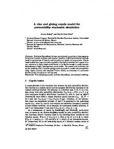
Fig. 5. Results of a series of F-tests to evaluate the effect of increasing the amount of information into the models on the variance. A, proportion cover for the four vegetation-cover types; B, pixel-by-pixel percent agreement; C, edge; and D, contagion (P < Fa.05; dfpixe, - 9,9; dfpixe, vs owner = 9 3 ; dfpatch vs owner = 1999; dfowner = 19,19).
model and largest in the patch model. The addition of information in the model formulations did not yield obvious changes in variance as it did with the means. The variance in the 4 and 5-data layer treatments for both model types were never significantly different from each other, and usually significantly different from those treatments with the lowest number of data layers. The relationship between variance and informational content was weaker still with percent agreement, contagion, and edge, but significant difference between the 4 and 5 data layer simulations and those with the least amount of information were present most of the time (Fig. 5b-d). Discussion Pixel and patch-based approaches to stochastic spatially-explicit modeling of landscape change in human-dominated landscapes were examined.
Both approaches simulated changes in proportion cover and percent agreement equally well. However, only the patch-based model with ownership boundaries captured the complexitiy of the spatial pattern of the landscape. In fact, measures of spatial pattern, contagion and edge, calculated from the 5-data-layer pixel and patch simulations were often significantly different from those of the simulations that incorporated ownership boundaries. This study demonstrated that the scale of transition must be identified if the spatial structure of a landscape is to be simulated adequately. Each model formulation implemented transitions at a different scale. In the simulations, vegetation changes occurred at scales that were either too fine (pixel-based model) or too broad (patch-based model), even when five data themes were used to construct their transition matrices. The ownership model, which served as a basis of comparison for the other formulations, succeeded because its
45
vegetation-cover changes used the same information (5 data themes and ownership boundaries) and, therefore, occurred at a similar scale as those that produced the VEGCOVER2 map. Adding empirically-derived information significantly improved the representation of spatial patterns of pixel- and patch-based models. In the pixelbased model, the scale of transition that produced the VEGCOVER2 maps was being approximated through the coalescence of individual pixels with increasing information. In the patch-based model, large groups of contiguous pixels were reduced in size with added information and began to reflect the scale of change that produced VEGCOVER2. Although both pixel and patch-based models can reflect spatial patterns of landscape change, the patch-based approach can probably do so with less additional information because attributes of landscape structure are represented in patch size, shape, and juxtoposition. Adding information to the models also decreased the variance of all measures. Variance can serve as a source of error propagation and may be of serious concern if multiple time steps are run (Gardner et al. 1990). For stochastic land-use models, multiple time steps in a single simulation will be a reality as dynamic transition probabilities are implemented (Lee et al. 1992). Therefore, future research that explores error propagation over multiple time steps remains a significant need. This study did not attempt to evaluate the impact of each spatial data theme on the model formulations. We recognized that the content of each data theme and the order of their incorporation into the models affected the simulation results. Some of the data themes provided little information about the landscape (LANDUSE) regardless of their position in the order, while others (OWNERCLASS) were a significant addition if placed at any position. DISTROAD and DISTCULT contained some common information, so that the contributions that these data layers made depended on which was inserted into the model first. It is unlikely that our conclusions about the two model formulations would be different if the data themes were introduced into the model in a different order. To demonstrate, this we ran simulations where the data themes OWNERCLASS, LANDUSE, DIS-
TROAD, DISTCULT were incorporated into the model in the opposite order as before. The results were basically the same; no significant difference for model type and information detail for proportion cover, while the spatial measures differed by model type and information content. Characterizing pixels and patches using landscape condition labels proved to be an extremely versatile approach. Because the landscape-condition labels were represented as character strings, the benefits of this approach included (1) the landscape-condition-label’s length (e.g., the amount of information used in a simulation) was not limiting; (2) adding information into the model was facile, involving simply overlaying the new map layer and appending the new category value to the end of the existing landscape-condition label of each pixel; and (3) because the patches are constructed by aggregating pixels, patch size can be delineated by any set of map layers the modeler chooses. This approach provides an avenue to address, in a spatially explicit format , socioeconomic and environmental questions at the landscape scale. By employing a landscape-condition label and patch-based transitions, this model can simulate fine-scale landscapes changes at the scale of change as defined by human land use patterns. Output from this type of model could then be used to examine changes in the spatial quality of biotic (e.g. , species’ habitat requirements) and physical variables (e.g. , erosion) as well as feedbacks on human decision making caused by landscape change. In this paper, a stochastic model is presented in which ecological and socioeconomic variables are integrated to simulate landscape change. This integration is accomplished by representing all model inputs (variables and results of submodels) and conducting the simulation in a spatially-explicit manner. Since all model inputs are represented spatially, relational variables based on distance, adjacency, juxtaposition and patch shape can be derived and used as inputs as well. This approach provides a flexible environment for spatial simulation modeling and has several attributes including: (1) large-scale impacts to environmental and socioeconomic variables caused by landscape change can be evaluated and, (2) complex, landscape-level, feedback processes can be examined (Lee et al. 1992).
46 Acknowledgments
We thank J. Beauchamp for providing valuable statistical advice and V. Dale, R. Graham, R. Naiman, D. Wear and an anonymous reviewer for their critical review of the manuscript. This work was supported in part by the U.S. Man and Biosphere Program (No. 1753-000574); the appointment of R.O. Flamm to the U.S. Department of Energy Laboratory Cooperative Postgraduate Research Training Program administered by Oak Ridge Institute for Science and Education; and by the Ecological Research Division, Office of Health and Environmental Research, U S . Department of Energy, under Contract No. DE-AC05-840R21400 with Martin Marietta Energy Systems, Inc. Publication No. 4186, Environmental Sciences Division, Oak Ridge National Laboratory. References Baker, W.L. 1989. A review of models of landscape change. Landscape Ecol. 2(2): 111-133. Berry, J.K. and Sailor, J.K. 1987. Use of a geographic information system for storm runoff prediction from small urban watersheds. Environ. Manag. 11: 21-27. Boumans, R.M.J. and Sklar, F.H. 1990. A polygon-based spatial model for simulating landscape change. Landscape Ecol. 4: 83-97. Burnham, B.O. 1973. Markov intertemporal land use simulation model. S.J. Agric. Econ. 5: 253-258. Costanza, R., Sklar, F.H. and Day, J.W., Jr. 1986. Modeling spatial and temporal succession in the Atchafalaya/Terrebonne marsh estuarine complex in south Louisiana. In Estuarine Variability. pp. 387-404. Edited by D.A. Wolfe. Academic Press, New York, NY. Dale, V.H., Southworth, F., O’Neill, R.V., Rosen, A. and Frohn, R. 1993. Simulating spatial patterns of land-use in Rondonia, Brazil. In Some Mathematical Questions in Biology. pp. 29-56. Edited by R.H. Gardner. Am. Math. SOC., Providence, RI. De Roo, A.P.J., Hazelhoff, L. and Burrough, P.A. 1989. Soil erosion modelling using ‘ANSWERS’ and geographic information systems, Earth Surface Processes and Landforms 14: 517-532. Gardner, R.H., Dale, V.H. andO’Neil1, R.V. 1990. Error propagation and uncertainty in process modeling. In Process Modeling of Forest Growth Responses to Environmental Stress. pp. 208-219. Edited by R.K. Dixon, R.S. Meldahl, G.A. Ruark, and W.G. Warren. Portland, Oregon: Timber Press. Hall, F.G., Strebel, D.E. and Sellers, P.J. 1988. Linking knowledge among spatial and temporal scales: vegetation, atmosphere, climate and remote sensing. Landscape Ecol. 2(1): 3-22.
Hett, J. 1971. Land use changes in east Tennessee and a simulation model which describes these changes for 3 counties. ORNL-IBP-71-8. Oak Ridge National Laboratory, Oak Ridge, TN. Horn, H.S. 1976. Markovian properties of forest succession. In Ecology and Evolution of Communities. pp. 196-211. Edited by M.L. Cody and J.M. Diamond. Harvard Univ. Press, Cambridge, MA. Kadlec, R.H. and Hammer, D.E. 1988. Modeling nutrient behavior in wetlands. Ecol. Model. 40: 37-66. Kessel, S.R. 1977. Gradient modeling: a new approach to fire modeling and resource management. In Ecosystem Modeling in Theory and Practice. pp. 576-605. Edited by C.A.S. Hall and J.W. Day, Jr. Wiley-Interscience, New York, NY. Lee, R.G., Flamm, R.O., Turner, M.G., Bledsoe, C., Chandler, P., DeFerrare, C., Gottfried, R., Naiman, R.J., Schumaker, N. and Wear, D. 1992. Integrating sustainable development and environmental vitality: a landscape ecology approach. In Watershed Management: Balancing Sustainability and Environmental Change. Edited by R. J. Naiman. SpringerVerlag, New York, New York. Lippe, E., De Smidt, J.T. and Glenn-Lewin, D.C. 1985. Markov models and succession: a test from a heathland in the Netherlands. J. Ecol. 73: 775-791. Parks, P.J, 1990. Models of forested and agricultural landscapes: integrating economics. In Quantitative Methods in Landscape Ecology. pp. 309-322. Edited by M.G. Turner and R.H. Gardner. Springer-Verlag, New York, NY. Show, I.T., Jr. 1979. Plankton community and physical environment simulation for the Gulf of Mexico region. In Proceedings of the 1979 Summer Computer Simulation Conference. pp. 432-439. Society for Computer Simulation, San Diego, CA. Sklar, F.H., Costanza, R. and Day, J.W. Jr. 1985. Dynamic spatial simulation modeling of coastal wetland habitat succession. Ecol. Model. 29: 261-281. Sklar, F.H. and Costanza, R. 1990. The development of dynamic spatial models for landscape ecology: a review and prognosis. In Quantitative Methods in Landscape Ecology. pp. 309-322. Edited by M.G. Turner and R.H. Gardner. Springer-Verlag, New York, NY. Southworth, F., Dale, V.H., O’Neill, R.V. 1991. Contrasting patterns of land use in Rondonia, Brazil: simulating the effects on carbon release. Internat. Social J. 130: 681-698. Steel, R.G.D. and Torrie, J.H. 1960. Principles and Procedures of Statistics. McGraw-Hill, New York, NY. Turner, M.G. 1987. Spatial simulation of landscape changes in Georgia: a comparison of 3 transition models. Landscape E d . 1: 29-36. Turner, M.G. 1988. A spatial simulation model of land use changes in a piedmont county Georgia. Appl. Math. Comput. 27: 39-51. Turner, M.G. and Gardner, R.H. 1990. Quantitative Methods in Landscape Ecology. Springer-Verlag, New York, NY. Turner, M.G., Costanza, R. and Sklar, F.H. 1989. Methods to evaluate the performance of spatial simulation models. Ecol. Model. 48: 1-18.