A stochastic model for the spatial‐temporal simulation of ...

WATER RESOURCES RESEARCH, VOL. 46, W11501, doi:10.1029/2009WR008884, 2010

A stochastic model for the spatial‐temporal simulation of nonhomogeneous rainfall occurrence and amounts A. Burton,1 H. J. Fowler,1 C. G. Kilsby,1 and P. E. O’Connell1 Received 9 November 2009; revised 3 June 2010; accepted 15 June 2010; published 2 November 2010.

[1] The nonhomogeneous spatial activation of raincells (NSAR) model is presented which provides a continuous spatial‐temporal stochastic simulation of rainfall exhibiting spatial nonstationarity in both amounts and occurrence. Spatial nonstationarity of simulated rainfall is important for hydrological modeling of mountainous catchments where orographic effects on precipitation are strong. Such simulated rainfall fields support the current trend toward distributed hydrological modeling. The NSAR model extends the Spatial Temporal Neyman‐Scott Rectangular Pulses (STNSRP) model, which has a homogeneous occurrence process, by generating raincells with a spatially nonhomogeneous Poisson process. An algorithm to simulate nonhomogeneous raincell occurrence is devised. This utilizes a new efficient and accurate algorithm to simulate raincells from an infinite 2‐D Poisson process, in which only raincells relevant to the application are simulated. A 4009 km2 Pyrenean catchment exhibiting extreme orographic effects provides a suitable case study comprising seven daily rain gauge records with hourly properties estimated using regional downscaling relationships. Both the NSAR and the STNSRP models are fitted to five calibration rain gauges. Simulated hourly fields are validated using the remaining two rain gauges providing the first validation of time series sampled from STNSRP or NSAR processes at locations not used in model fitting. The NSAR model exhibits considerable improvement over the STNSRP model particularly with respect to nonhomogeneous rainfall occurrence at both daily and hourly resolutions. Further, the NSAR simulation provides an excellent match to the spatially nonhomogeneous observed daily mean, proportion dry, variance, coefficient of variation, autocorrelation, skewness coefficient, cross correlation and extremes, and to the hourly proportion dry and variance properties. Citation: Burton, A., H. J. Fowler, C. G. Kilsby, and P. E. O’Connell (2010), A stochastic model for the spatial‐temporal simulation of nonhomogeneous rainfall occurrence and amounts, Water Resour. Res., 46, W11501, doi:10.1029/2009WR008884.

1. Introduction [2] As catchment size increases, both rainfall amounts and occurrence become more spatially variable until modeling assumptions of spatial homogeneity of rainfall become unsuitable for hydrological applications [e.g., Fowler et al., 2005]. This increased variability is often due to the interaction of mountainous terrain with the atmosphere, creating orographic effects, which typically include increased rainfall amounts and occurrence on the windward side of mountains and reduced amounts and occurrence downwind [e.g., see Hill et al., 1981; Wheater et al., 2000; Barros and Lettenmaier, 1993, 1994; Roe, 2005]. [3] Stochastic models of rainfall in mountainous catchments are needed for hydrology, e.g., Barros and Lettenmaier [1993] report that 70% of annual runoff in the western

1 Water Resource Systems Research Laboratory, School of Civil Engineering and Geosciences, Newcastle University, Newcastle Upon Tyne, UK.

Copyright 2010 by the American Geophysical Union. 0043‐1397/10/2009WR008884

United States is disproportionately controlled by the duration and distribution of high elevation precipitation. In addition to amounts, the simulation of realistic rainfall occurrence is important because runoff generation is nonlinear (i.e., the same rainfall depth in fewer days produces higher runoff) and when conditioning a stochastic weather generator [e.g., Wilks and Wilby, 1999; Kilsby et al., 2007] occurrence is crucial as wet days are cooler and have lower potential evapotranspiration than dry days. [4] A number of multisite methodologies exist that can simultaneously simulate differing expected amounts and occurrence at a finite number of rain gauges: multisite Markov chains [e.g., Wilks, 1998; Mehrotra and Sharma, 2007; Srikanthan and Pegram, 2009], multivariate autoregressive approaches [e.g., Bárdossy and Plate, 1992; Stehlík and Bárdossy, 2002], generalized linear models (GLMs) [e.g., Chandler and Wheater, 2002; Segond et al., 2006], resampling from historical records using K‐nearest neighbors (KNN) [Buishand and Brandsma, 2001], GLM plus KNN [Mezghani and Hingray, 2009] and best match to rainfall probability and mean rainfall amount estimated using regression of atmospheric state variables [Wilby et al., 2003]. However, Markov chain and autoregressive models may have a large number of parameters and the resampling

W11501

1 of 19

W11501

BURTON ET AL.: THE NSAR STOCHASTIC RAINFALL MODEL

schemes cannot generate spatial rainfall patterns that have not been observed in the historical record. Further, these methodologies typically generate time series with daily time steps and at a finite number of locations (rather than generating spatial fields). Exceptions include the potential to spatially interpolate the GLM methodologies (with a potential loss of spatial heterogeneity) and the Mezghani and Hingray [2009] resampling of daily sets of hourly data, albeit with an underestimate of autocorrelation (at 6 h daily aggregation levels) and a limitation of repeating subdaily multisite patterns seen in the observed record. [5] However, the current trend toward distributed hydrological modeling requires continuous spatial rainfall fields to capture heterogeneities and subdaily time steps for rapid processes. Spatial extensions to point process stochastic rainfall models such as the BLRP or NSRP models [e.g., Cowpertwait, 1995; Onof et al., 2000] provide the requisite continuous temporal and spatial simulation processes that can be sampled at arbitrary temporal aggregations (e.g., hourly), spatial integrations (e.g., for the grid squares of a distributed model), or spatial locations (e.g., at rain gauge network locations or grid nodes). Additionally, such approaches can be easily reparameterized and used to downscale climate change scenarios [e.g., Kilsby et al., 2007]. [6] The Spatial Temporal Neyman‐Scott Rectangular Pulses (STNSRP) model [e.g., Burton et al., 2008] was formulated analytically by Cowpertwait [1995], extending the single‐site NSRP process [Rodriguez‐Iturbe et al., 1987]. This model has a spatially heterogeneous amounts process to account for orographic enhancement but is limited to a homogeneous occurrence process. The STNSRP model has been demonstrated in a number of practical applications [e.g., Cowpertwait et al., 2002; Fowler et al., 2005; Burton et al., 2008]. However, for a downscaling application to a 15,000 km2 region in Yorkshire, UK, Fowler et al. [2005] found it necessary to develop two separate subregional rainfall models to reduce the modeling errors arising from the assumption of spatial homogeneity in rainfall occurrence. [7] Orographic effects lead to an increase in the number and duration of precipitation events [Barros and Lettenmaier, 1994] and rainfall in mountains is associated with the passage of preexisting precipitation systems, some of which may be too slight to be recorded by upwind rain gauges [Hill et al., 1981]. These observations suggest two possible modifications of the spatial BLRP or spatial NSRP models to account for nonhomogeneous orographic effects: (1) modifying the storm incidence process; (2) modifying the number, properties or behavior of the raincells. The former may be more appropriate where the type of event giving rise to rainfall varies spatially, as may happen over a large region, and the latter when large scale events trigger local rainfall in accordance with the physical geographical setting. [8] Following the latter alternative Cowpertwait [1995] suggested a possible analytical extension to the STNSRP model to represent spatially heterogeneous rainfall occurrence for a multisite application. Each sample location was considered to have an associated survival probability which modulated a homogeneous STNSRP raincell generation process. A raincell may therefore be observed at some locations and not at others across its disc. While such an approach is analytically appealing, no application of such a model has been demonstrated and it is not clear if the pro-

W11501

cedure can be extended to a spatial process. An approach based on the single‐site NSRP process was however demonstrated by Favre et al. [2002]. Simulated storms followed a master Poisson process, but raincells were generated at two rain gauges using bivariate distributions of number, intensity, and duration. Fitting yielded models with different expected numbers of raincells and the ability to simulate different precipitation occurrence probabilities at each rain gauge. Generalization of this approach to more sample locations may not be straightforward. Wheater et al. [2000] also provided an extension to the spatial BLRP model where the mean duration of raincells was adjusted spatially. Nonhomogeneous amounts and hourly occurrence were well fitted. However, the fit to daily and 6 hourly occurrences was typically biased low and the spatial nonstationarity of the daily and 6 hourly occurrence was not well modeled. [9] Here the nonhomogeneous spatial activation of raincells (NSAR) model is developed and demonstrated to provide a single process which addresses the need for stochastic models able to simulate continuous spatial‐temporal rainfall with spatially heterogeneous occurrence and amounts properties. This is achieved by extending the STNSRP model so that raincell occurrence within storms follows a spatially nonhomogeneous Poisson process.

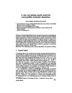
2. The NSAR Model Structure [10] The spatial‐temporal NSAR model provides a stochastic conceptualization of rainfall in which a sequence of “storm events,” each of which may represent for example frontal rainfall or a mesoscale convective system, provide spatially large scale initiation of localized rainfall. Such localized rainfall exhibits both high variability and short range correlation in both space and time. Orographic enhancement may also significantly affect both the occurrence and amounts of rainfall at specific locations. For hourly and daily temporal scales and for spatial scales from point to ∼10,000 km2 the localized rainfall is conceptualized as occurring as circular raincells with uniform intensity throughout their lifetime and extent. These are distributed unevenly across the region of interest to account for geographic location effects on rainfall occurrence and clustered in time following each storm event. A final scaling of raincell intensity further accounts for location specific effects on rainfall amounts. [11] The stochastic model structure is illustrated in Figure 1 and its detailed construction follows. [12] 1. Storm events are modeled as storm origins, instants at which spatially large scale triggers of raincell events occur. Storm origins occur following a stationary Poisson process in time with rate l (1/h). [13] 2. Each storm origin generates a set of immobile circular raincells whose centers follow a nonhomogeneous spatial Poisson process, with density r(x) (1/km2) over an infinite planar simulation region x2R2, and whose radii are exponentially distributed, with parameter g (1/km). [14] 3. Each raincell begins producing rainfall at its origin time, which follows the storm origin after a waiting time interval. Waiting time is exponentially distributed with parameter b (1/h). [15] 4. Each raincell produces a uniform rainfall rate across its disc and throughout its lifetime. The duration and

2 of 19

W11501

BURTON ET AL.: THE NSAR STOCHASTIC RAINFALL MODEL

Figure 1. The conceptual structure of the stochastic NSAR model shown by means of a possible realization which is sampled at two rain gauges m1 and m2. Steps are labeled (1–5) (1) a time series of storm origins; (2) the spatially nonhomogeneous distribution of raincells generated by one such storm origin over a hypothetical catchment; (3) time series of raincell origins relevant to each rain gauge for this storm; (4) intensity and duration properties of these raincells; (5) scaled intensity time series generated at each rain gauge.

the intensity of the raincell are exponentially distributed with parameters h (1/h) and x (h/mm), respectively. [16] 5. The rainfall intensity field at any instant is the sum of the intensities of all active raincells scaled by a spatially nonuniform intensity scaling field, y(x). This field models geographically varying raincell intensities. [17] Time series of spatially distributed fields of accumulated rainfall depths may be obtained numerically by integrating the intensity field over regular time steps for a grid of sampling locations. Similarly, multisite time series may be obtained by sampling the process at several locations, e.g., corresponding to rain gauges, and integrating the field over regular time steps. The NSAR model’s parameters are summarized in Table 1 and consist of five parameters and two fields {l,b,r(x),g,h,x,y(x)} all of which are nonnegative. Different parameterizations for each calendar month provide an annual cycle of rainfall properties. [18] The new NSAR model is developed from the STNSRP stochastic rainfall model described by Cowpertwait [1995] and Burton et al. [2008]. Both models utilize a nonuniform intensity scaling field which models spatially varying rainfall amounts. However, the models differ in that the STNSRP model uses a homogeneous Poisson process to generate raincells in space with a uniform parameter r in step 2. Consequently rainfall occurrence is simulated as a spatially homogeneous process which takes no account of geographic effects and for each month the STNSRP model is parameterized by six parameters and one field {l,b,r,g,h,x,y(x)} (see Table 1). In contrast, the new

W11501

methodology has the advantage that varying incidence of raincells at different geographic locations can additionally model spatially varying rainfall occurrence and storm duration. Both the NSAR and the STNSRP models provide a simplistic stochastic representation of the rainfall process: for example, raincells do not move and have a simplistic geometry, and storms are all considered to arise from the same process. However, the STNSRP process has been found useful at the spatial and temporal scales of particular relevance to hydrological investigations of catchments of up to ∼10,000km2 [see Burton et al., 2008]. [19] In the single‐site NSRP process [e.g., Cowpertwait, 1991], the sampling of spatial properties, step 2, is omitted altogether and instead the number of raincells that affect the single rain gauge may be sampled directly for each storm (a Poisson random variable with mean n). Typically step 5 is also omitted as it is redundant. So for each month the NSRP model has five parameters {l,b,n,h,x}. Here, however, it is convenient to consider an NSRP process at a location xm with intensity field scaling (i.e., atypically including step 5) which has the six parameters {l,b,n,h,x,y m} where y m ≡ y(xm) (see Table 1). A useful property of this model [e.g., Cowpertwait, 1995] is that it is equivalent to an STNSRP process sampled at location xm provided common parameters are equal and
¼

2 : 2

ð1Þ

3. Fitting the NSAR Model 3.1. Fitting the STNSRP Model [20] The fitting scheme of the NSAR model uses many properties of the STNSRP model and so the STNSRP fitting procedure is briefly summarized. First the intensity scaling field, y(x), is estimated at rain gauge locations {xm} in proportion to the mean daily rainfall, producing the vector Y ≡ [y m] ≡ [y(xm)]. During a spatial simulation the intensity scaling field may be estimated by interpolation of these values so that the full STNSRP process is parameterized by {l,b,r,g,h,x,Y}, (6 + M) parameters where M is the number of rain gauges, for each calendar month in turn. The same parameter set is used for multisite simulations, where time series are sampled at rain gauge record locations, but interpolation of the field is unnecessary [e.g., Cowpertwait, 1995; Cowpertwait et al., 2002]. [21] Second, a numerical optimization scheme is used to find the best choice of the remaining parameters to minimize an objective function, equation (2) [see Burton et al., 2008], which describes the degree to which a simulation is expected to correspond to observed rainfall statistics for a given month, Dð; ; ; ; ; j YÞ ¼

X w2g g2W

gs2

ðg^  g ð; ; ; ; ; ; YÞÞ2 ; ð2Þ

where W is the set of rainfall statistics each with an aggregation period and a location (such as 24 h variance at rain gauge m2), g^ is the observed sample estimate of each statistic, and g(·) is the corresponding expected statistic from the simulation process expressed analytically in terms of the model’s parameters. The weight applied to each statistic wg is set by the user to control the relative accuracy with which

3 of 19

W11501

W11501

BURTON ET AL.: THE NSAR STOCHASTIC RAINFALL MODEL Table 1. The Parameters of the NSAR, STNRSP, and NSRP Models as Described in the Texta Parameter or Field

Model Usage NSAR

STNSRP

NSRP

Description

Unit

• • •

• •

• •

Storm origin arrival rate 1/(mean waiting time) Spatially varying raincell density field Uniform raincell density field Number of raincells affecting a rain gauge 1/(mean raincell radius) 1/(mean raincell duration) 1/(mean raincell intensity) Spatially varying intensity scaling field Intensity scaling at a specific location

(1/h) (1/h) (1/km2) (1/km2) (−) (1/km) (1/h) (h/mm) (−) (−)

l b r(x) r n g h x y(x) ym

•

• • • •

• • • •

• • • •

Circles indicate the parameters used by each model. The fields r(x) and y(x) are functions of location, x.

a

each statistic is fitted, in accordance with the uncertainty of each observed statistic or as most appropriate for a particular hydrological application. The scaling term gs is either one for a probability dry or correlation statistic or the annual mean of the statistic. Analytical expressions for g(·) are available for expected statistics of any accumulation period of the STNSRP process at any location: for the mean, variance, lag‐ autocovariance and probability of a dry period (PDry) by Cowpertwait [1995]; dry‐dry and wet‐wet transition probabilities by Cowpertwait [1994]; and the third order central moment by Cowpertwait [1998]. Expressions relating the expected covariance between two locations are also available [Cowpertwait, 1995]. For the model to be identifiable W must include at least the same number of statistics as there are parameters to be fitted, both first and second order statistics, PDry and cross‐correlation, and either the transition probabilities or the autocorrelation. 3.2. Analytical Properties of the NSAR Model [22] The vector Y is used to parameterize the NSAR model’s intensity scaling field as for the STNSRP model. Similarly the spatially varying raincell density field is characterized by point values rm at nodes positioned at the locations {xm} of the M rain gauges. The NSAR model parameterization is then {l,b,r,g,h,x,Y}, where r ≡ [rm], requiring a total of (5 + 2M) parameters. The raincell density field has a more complex influence on the expected statistics of the model than the intensity scaling field, and so it is necessary to specify the form of the spatial interpolation used prior to fitting the model. Interpolation of nodal values using inverse square distance was chosen as it is a simple scheme which provides a smooth but responsive density field, r(x∣r), at any location x. The interpolated field is given by equation (3) with interpolation weights given by equation (4). ðx j rÞ ¼

M X

[23] Analytical expressions for the expected statistics of the NSAR process sampled at any point are now derived in terms of the expressions available for the STNSRP process. The NSAR process generates the storm origin and the raincell origin, duration, intensity, and radius in the same way as for the STNSRP process. Both the NSAR and the STNSRP models’ Poisson raincell generation processes lead to a Poisson random number of raincells that all influence a rain gauge located at x, Cx. However, for the NSAR model Cx is nonhomogeneous in space whereas for the STNSRP model it is homogeneous. The NSAR process sampled at x is therefore equivalent to an NSRP process at x with common parameters equal and n = E(Cx). An STNSRP process sampled at x, with common parameters equal, is also equivalent provided r, n, and g are related by equation (1). [24] The probability of a raincell with center x and exponentially distributed radius (with parameter g) influencing a rain gauge at xm is the survivor function of the radius random variable at the distance ∣x−xm∣, i.e., the probability of the radius being greater than the distance from x to xm. The expected number of raincells reaching xm, E(Cxm), in a storm due to raincells with centers following a nonhomogeneous 2‐D Poisson process defined by r(x∣r) may then be evaluated as ZZ EðCxm Þ ¼

[25] Equations (3), (4), and (5) may be combined and the order of integration and summation swapped to obtain an expression for the NSRP raincell number parameter at rain gauge m equivalent to the NSAR process sampled there,
m ð; rÞ ¼

wm ðxÞm ;

ð3Þ

M X

amn ð Þn ;

ð6Þ

ejxxm j j x  xn j2 dx M P ðj x  xk j2 Þ

ð7Þ

where ZZ amn ð Þ ¼

j x  xm j2 : M P ðj x  xk j2 Þ k¼1

ð5Þ

x2