Ambiguity Aversion in the Brain - CiteSeerX

Ambiguity Aversion in the Brain Ming Hsu June 9, 2004

1

Introduction

The distinction between “ambiguity” on the one hand, the “risk” on the other, has been a long standing one in both economics, statistics, and probability theory. The former refers to situations where the decision-maker can assign numerical probabilities to the states at hand, the latter to situations when the various states of nature cannot be expressed in terms of “objective” probabilities. This is also the problem of multiple prior distributions in statistics, especially Bayesian and neo-Bayesian methods. Indeed, Bayesian methods have often been criticized on grounds that they does not provide an intuitively appealing method to handle non-unique prior distributions1 . There are many, however, who think the distinction to be more heat than light—that ambiguity doesn’t matter—that is, holding beliefs constant, the amount of evidence used to form the belief is (or should be) irrelevant. On the other hand, there are many models about how and why ambiguity should matter. This paper approaches this problem by imaging the brain (using fMRI) when people make both types of decisions. If ambiguity does not matter, then the same brain regions should be activated in risky and ambiguous decision. If ambiguity does matter, then differences in regional activation can provide empirical constraint about which theories are on the right track. The latter is especially valuable given the difficulty past behavioral experiments have had separating the various models. The economic applications of ambiguity is potentially vast. “Objective” probabilities, with the exception of certain games of chance, rarely exist. Knight suggested that entrepreneurs are compensated for bearing uncertainty rather than risk [34]. Ambiguity has also been invoked to explain such phenomenon as the equity premium, home bias, overinsurance, etc. [16] [18]. Recently macroeconomists have begun exploring carefully the implications of policy-maker ambiguity about whether they have the right model of the economy (e.g. [26]). Indeed, Phelps [45] mentions this concept as central in his early thinking in his invention of the “islands model” later used by Lucas and others, but notes how it was neglected by theorists who followed. The organization of the paper is as follows: Section 2 describes the basic issues and empirical regularities discovered in experiments of decision making under ambiguity. Section 3 discusses the various theoretical models, and relates them to possible regions of neural activation. Section 4 gives a brief overview of what is known about the areas relevant to debates in decision making, and explored more fully in the discussion. Section 5 discusses previous imaging studies of decision making under ambiguity. Section 6 discusses the experimental design. Section ?? describes results2 . Section 8 summarizes and concludes. Two appendices are also included. Appendix A surveys some methods and technical matters in neuroscience for readers unfamiliar with this field. Appendix B includes ancillary design details. Appendix C contains the details figures referenced in the results section. 1 These two paths converged in the form of Gilboa & Schmeidler with maxmin expected utility in economics, and Wald in statistics. 2 A number of the figures were relegated to the end of the document by LaTex. Sorry.

1

2

Ellsberg Paradox

The distinct between ambiguity and risk is not one recognized by standard subjective expected utility theory first presented by Ramsey and de Finetti, and axiomatized by Savage.3 This was the grounds for Ellsberg’s famous thought experiment. He proposed the following. Axiom 1 Urns A and B each have 100 balls each of either red or black. Urn A contains 50 red balls and 50 black ones, whereas there was no additional information about urn B. One ball is to be drawn from each urn. Call bet AR “the ball from urn A is red”; bet AB “the ball from urn A is black, and similarly for BR and BB . Winning a bet earns the decision maker to, say, $10. In this problem, there are four states: (IB, IIB), (IB, IIR), (IR, IIB), (IB, IIR). The deterministic outcomes are the money earned. The bet AR is an act which assigns the (degenerate objective) lottery of receiving “$10 with probability one” in the event IR, and “$0 with probability 1” in the event IB. Indifference between these two acts, plus independence, continuity, and weak order imply indifference between these two acts and a constant act over an objective (roulette) 50-50 lottery for $10 and $0. Likewise, the same argument holds for IIR and IIB. Taken together, they imply indifference between all four bets. Ellsberg also proposed another version, commonly called the 3-color urn. Axiom 2 An urn contains 90 balls. There are 30 red (R). The other 60 are either black (B) or yellow (Y), but of unknown numbers of each. One ball will be drawn at random from the urn. There are 4 bets A1 $100 if R, otherwise $0. A2 $100 if B, otherwise $0. B1 $100 if R or Y , otherwise $0. B2 $100 if Y or B, otherwise $0. He predicted that many decision makers will choose A1 over A2 , but B2 to B1 . This would show the decision maker violating an even more fundamental decision rule—first order stochastic dominance (FOSD). Definition 3 (First Order Stochastic Dominance) Let FA (x) be the probability of winning not more than x in lottery A. If for every x, FA (x) ≤ FB (x), then lottery A is (weakly) preferred to lottery B. 3

Here I will mostly use the simplication of the Savage model by Anscombe and Aumann [1].

2

Denote the lotteries by f = (x, S; 0, ¬S), where x and 0 are the prizes, and S the state. By FOSD, the lottery (x, S; 0, ¬S) is preferred to (x, T ; 0, ¬T ) iff the subjective probability of S is greater than that of T . In the above, P (R) = 31 , P (B ∪ Y ) = 32 . Preferring A1 over A2 implies P (R) = 13 > P (B), but P (R ∪ Y ) = 1 − P (B) > 32 = P (B ∪ Y ). As FOSD is one of the most basic criterion in decision making, ambiguity aversion is much more damning to SEU than violating the independence axiom, which many find objectionable.

2.1

Behavioral Experiments

Ellsberg presented his problem as a thought experiment, but his predictions have been replicated in numerous experiments. A non-trivial proportion of subjects exhibit preferences AB ∼ AR Â BB ∼ BR [5] [36] (for a detailed review see Camerer and Weber [10]). Ambiguity premium is typically around 20% of the expected value of the gamble. In addition to Ellsberg’s original problem, ambiguity aversion has been replicated across a variety of settings. Fox and Tversky [20] asked questions such as “Was the temperature of San Francisco two weeks ago above 70 degrees?” or “Was the temperature of Istanbul two weeks ago above 70 degrees?” They reasoned that subjects, who were undergraduates at Stanford and other US colleges, would be more familiar with the temperature of San Francisco compared to those of Istanbul, but the actual probability of getting the bet correct is similar for both questions. Indeed, they found that subjects preferred the bet on which they had more knowledge—San Francisco, versus Istanbul. Their study also has the advantage that it is clearly a game against nature, and that, unlike the balls in urn problem, the experimenter cannot rig the experiment against the subject. Ambiguity aversion also appears to be immune to market institutions. Camerer and Kunreuther created a simple market for insurance [11]. They found that, although ambiguity did not have a systematic effect on prices, it did increase the number of losses insured by the insurer. Sarin and Weber used experimental markets with German business students and bankers [53]. The price for a known 0.5 bet was significantly larger than that of the ambiguous bet. Bossaerts et al. found that, in financial market experiments with risky and ambiguous states, the prices and holdings of assets reflect substantial ambiguity aversion [9]. Ambiguity aversion also appears to be immune to persuasion. This is important as it has been argued on grounds that there “ought not” be any difference between risk and ambiguity, and that exhibiting behavior to the contrary is a form of “mistake.” Slovic and Tversky showed the three-color Ellsberg problem to 49 students after having them read two statements before making choice. One statement explained the independence axiom, whereas the other explained the psychological appeal of ambiguity aversion. Eighty percent of subjects committed the paradox. In fact, most subjects found the statement advocating ambiguity aversion more compelling [62].

3

3

Theoretical Literature

A number of models have been proposed over the years to account for ambiguity aversion in economics and the problem of multiple prior distributions in statistics. Here I will distinguish between two approaches in modeling ambiguity. One is to modify the expression of probabilities in SEU [57] [24] [61]. This “probability-based approach” usually uses decision weights using some modification of probabilities, which may or may not obey the usual rules of probability. Most models of ambiguity aversion fall in this category. Another approach is to allow utilities to differ under ambiguous and unambiguous situations [64] [21]. Ambiguity aversion then is consistent with the case where utility from ambiguous events is lower. Such state-dependent utility models are straight forward, but they are often unappreciated. Like the civic duty explanation for voter turn-out, these models tend to be ad hoc, and cannot explain a number of empirical facts unless built directly into the utilities4 . Yet they are not necessarily wrong. In fact the difficulty in testing them behaviorally is one of the reasons why it may be helpful to have fMRI studies. 3.0.1

Probability-Based Approach

Sub-additive Probabilities Schmeidler (1989) approached the problem by using subadditive probabilities—capacities, and weakening the independence axiom with the following version [57]. Axiom 4 (Comonotonic Independence) For all pair-wise co-monotonic acts f, g and h in L and for all α in (0, 1) : f  g implies αf + (1 − α)h  αg + (1 − α)h, where two acts f and g are said to be co-monotonic if for no s and t in state space S, f (s)  f (t) and g(t)  g(s). The rationale behind this setup is given by Schmeidler . . . if each of the symmetric and complementary uncertainty events is assigned the index 3/7, the number 1/7, 1/7=1-(3/7+3/7), would indicate the decision maker’s confidence in the probability assessment. Thus, allowing nonadditive. . . probabilities enables transmission or recording of information that additive probabilities cannot represent [57]. It was proved under the these assumptions that, if a preference relation satisfies the above properties, then there is a unique nonadditive probability v and a utility function u such that Z Z f % g iff u (f (·)) dv ≥ u(g(·))dv. S

S

Under this model, subjects who are ambiguity aversion assign probability of pr = pb < 1/2 for the red and black balls, respectively. It is easy to see then that U (BR) = U (BB) < U (AR) = U (AB). 4

For example, it is difficult for the utility based models to explain ambiguity aversion across various probability levels.

4

Maximin Expected Utility was introduced by Gilboa and Schmeidler5 [24]. Similar to Schmeidler [57], Gilboa and Schmeidler replaced the independence axiom with a weaker version. Axiom 5 (Certainty-Independence) For all f, g ∈ L and h ∈ Lc , where Lc is the set of constant acts, and ∀α ∈ (0, 1), f  g iff αf + (1 − α)h  αg + (1 − α)h. In addition, they included the uncertainty aversion axiom, which states that decision makers prefer a mixture of acts with objective probabilities over the acts themselves. Axiom 6 (Uncertainty Aversion) For all f, g ∈ L and α ∈ (0, 1), f ∼ g implies αf + (1 − α)g % f . The standard independence axiom is stronger than certainty independence in that it allows h to be any act in L rather than restricting it to constant acts Lc . They proved that under standard conditions with the aforementioned changes, the preference relation is represented by a function J(f ) up to a unique affine transformation. ½Z ¾ J(f ) = min u ◦ f dP |P ∈ C where f is an act, u is a von-Neuman-Mongenstern utility function over outcomes, and C a closed and convex set of finitely additive probability measures on the states of nature. Thus, it is easy to see why the decision maker would prefer urn I to II in the Ellsberg paradox. In particular, since C is the complete set of finitely additive probability measures on the states of nature, the distributions (black = 0, red = 100), and (black = 100, red = 100) are included. Second Order Priors A number of models have used the idea of a second-order prior. Through this method they are able to retain the independence axiom, but relax the reduction of compound lottery assumption. Indeed, there is evidence that subjects often violate the reduction assumption, especially when the stages are well separated [31] [48]. All of these models work by allowing the decision maker weight the probabilities nonlinearly (e.g., Segal [61]. Overweighting of the lower payoff acts by definition under-weights those with higher payoffs, thus resulting in ambiguity aversion. The opposite weighting results in ambiguity loving behavior. 5

This is similar to Wald in statistical theory, who noted A minimax solution seems, in general, to be a reasonable solution of the decision problem when an a priori distribution in Ω does not exist or is unknown to the experimenter [66].

5

3.0.2

Utility-Based Approach

The utility based models, as mentioned above, borders on tautology. If utility from winning an ambiguous bet is lower, ambiguity aversion is observed, e.g., Smith [64]. More sophisticated models have incorporated concepts such as regret into the utility based approach. In Rakesh and Winkler [?], decision makers dislike betting on the ambiguous urn because the disutility resulting from regret by the amount one could have won. They make the ad hoc assumption that there is no disappointment when the probabilities are know.

3.1

Neural Implications of the Previous Models

As reviewed above, the Ellsberg paradox provides a compelling objection to the axiomatic foundation behind SEU. Various writers have echoed this sentiment on grounds that certain axioms violate some of our intuitions about how a rational decision maker would behave. The following appeal to introspection is common in the literature on ambiguity aversion. ...consider the case where outcomes are real numbers and S = [0, 2π]. Let f and g be two acts defined: f (s) = sin(s) and g(s) = cos(s). The £ preferences ¤ f  g may be induced by the rough evaluation that the event π3 , 4π is more 3 probable than its complement. Define the act h by h(s) = sin(77s). In this case the structure of the acts f 0 = 21 f + 12 h and g 0 = 12 g + 12 h is far from transparent. Careful retrospection and comparison of the acts f 0 and g 0 may lead them to the ranking g 0  f 0 ... [57] Such “retrospection and comparison”6 is precisely what we hope to make precise. From a neural point of view, all of the above models have something in common: They predict that separate neural circuity will be activated when the odds are ambiguous, which lower the value of ambiguous gambles, either through the decision weights, or the utility of the gambles themselves. It is likely that the lower activation, under any of these models, will come in the form of signals of discomfort or negative emotion which are added to evaluations of the sort present in the risky case. Since this study is exploratory, if we find that there is differential activation in the ambiguity case that can be reliably described as negative emotion (due to implication of the activated regions in other studies which are reasonably described as activating negative emotion in other tasks) then we can conclude that some form of model which incorporates pessimism or lower utility is on the right track. 6

Gilboa and Schmeidler [24]: An intuitive objection to the standard independence axiom is that it ignores the phenomenon of hedging.

Segal [61]: It is my belief that decision makers consider the Ellsberg urn as a real two-stage lottery. . .

6

Understanding how the brain actually processes ambiguous situations can be especially useful for establishing evidence for utility based models. These models have been criticized, for good reason, for being ad hoc. Results from imaging, which has the potential of bypassing revealed preferences, can place constraints on state-dependent utilities that behavioral experiments can not. The central question facing neuroeconomics studies like this one is: How does knowing more about neural details affect the kinds of modelling we do in economics (since economic models of the individual necessarily abstract grossly from detail in order to provide a mathematical tool that can be aggregated)? One answer is that the brain regions will tell us about new types of variables that could affect expressed preferences. For example, if the insula is activated during ambiguity, then it is conceivable that when the insula is activated exogenously (e.g. by brief exposure to fearful or angry faces) then a player’s expressed preference changes. In decision theory language, the idea is that preferences may depend on internal states of the player (such as insula activation). Furthermore, this state-dependence will matter greatly in the economy if the internal states of people are jointly affected by a common shock (such as a war or malaise due to unemployment).

4

Neural Basis of Decision Making

Here I give a brief overview of the brain areas that have been found to be involved in decision making. More details will be found in the discussion.

4.1

Evaluation of Probabilities

Dopamine is a neurotransmitter that has been extensively studied in recent years, and is thought to be critically involved in reward learning and probability evaluation [60] [58] [59]. Most learning deficits are associated with damage to dopamine transmission in the NAcc [60]. The dopaminergic system consists of a number of subcortical nuclei, amongst which are the ventral tegmental areas (VT) and the nucleus accumbens (NAcc). These are associated with probability assessment [7] [35]. Work in monkey cell recordings show that dopamine neurons in the ventral tegmental area and substantia nigra represent prediction errors in the time and amount of reward [39]. There is also evidence that the NAcc activity is independent of reward value [7].

4.2

Utility of Reward

Nonlinearity in the utility function is an indication of risk attitudes. Elliot et al. shows that orbitofrontal cortex (OFC) responds nonlinearly to reward [17]. The OFC is a stretch of cortex situated in the ventral (bottom) surface of the brain, laying on top of the orbit bone. This is one of the areas suffering damage in Phineas Gage, a railroad worker who famously had an iron rod blasted through his head but miraculously survived with little impairment to his intelligence or memory. What did seem to be affected, however, was his social skills and 7

decision making abilities [27] [43]. This finding has been confirmed in other OFC patients over the past 80 years or so. One task that proved useful in diagnosing such patients is the so-called “gambling task” [4]. The task consists of the subject having to choose between 2 decks of cards for say, 100 trials. Deck I is composed of high returns and high losses, Deck II low returns and low losses. Overall Deck II dominates I in both mean and variance. The general finding of the task is that whereas most control subjects learn to choose only from Deck II, OFC patients persist in choosing from Deck I. It is important to note here that subjects are not told of the composition of the decks, and that the sampling is done without replacement, so the deck’s distribution is ambiguous. Clearly, the repeated nature (with feedback) of the experiment is a departure from the type of ambiguity present in the Ellsberg paradox. Subjects may hold different beliefs concerning the stationarity of the process7 . In terms of neuroanatomical connections, the OFC is in an ideal situation to integrate sensory input from other structures. All major sensory input—visual, auditory, somatosensory, gustatory, and especially olfactory—have some form of representation in the orbitofrontal cortex [40]. The close connection to the olfactory sensory inputs especially puts the OFC in a unique class amongst cortical areas. OFC neurons have been show to be selectively responsive to rewarding stimulus [50] [49]. In the monkey, the ensemble responds to appetitive stimuli, but stops when fed to satiety [15]. O’Doherty, using fMRI, found similar response in human OFC to appetitive odors when hungry, but not when satiated [41]. The OFC is also highly connected with the amygdala, an area important for fear processing and classical conditioning [43].

4.3

Expected Utility

Probability evaluation of state πs is independent of utility us of the reward under SEU8 . There is indeed evidence of this independence in areas of the brain that appear to evaluate probability and areas evaluating reward. Berns et al. showed in an fMRI study that the ventral striatum is activated independently of the reward value [7]. Platt and Glimcher found that neurons in the monkey LIP appears to track the expected value of the reward [46]. They showed that the LIP neurons respond linearly to both manipulations of probability and reward value. This however appears to be the exception rather than the rule. Most areas that respond to reward do not exhibit independence. This is perhaps not surprising, as a number of these areas are known to be involved in emotion and monitoring. One of those structures is the amygdala, a complex of nuclei situated at the end of the hippocampus. Amygdala neurons respond to primary rewards and reward predicting stimuli [60]. Its role in emotions and conditioning is well established, especially in the domain of fear. It is well documented that amygdala activity is not mediated by consciousness. In particular, 7

In fact, in a workshop I attended at George Mason University, a number of subjects, all of whom Ph.D. students in economics, persisted in choosing from the high variance deck, reasoning that “they [the experimenters] won’t let us walk away with losses.” Most subjects, however, do not exhibit this behavior. 8 Note that this is not true under minmax utility under Gilboa-Schmeidler.

8

the subliminal priming9 literature has shown convincingly that the amygdala will respond to emotional faces even though they are not consciously seen. The amygdala is crucially involved in learning [42]. Lesioning of the amygdala in rats impair associative learning. It is hypothesized on the basis of the strong reciprocal connections between the amygdala and the OFC, and a massive input from dopamine neurons, that the amygdala-OFC circuit is crucial in learning. Kahn et al. found that the amygdala was activated while subjects performed a variant of a matching game, in which there is a “safe choice” and “bluffing” [32]. They also found that the amygdala was most active during period after bluffing and the revealing of opponent’s choice. The orbitofrontal/insular cortex10 (FI), situated laterally next to the amygdala, is well noted for its role in decision making through studies across a variety of domains. This will be explored further in the discussion section.

5

Previous Imaging Studies

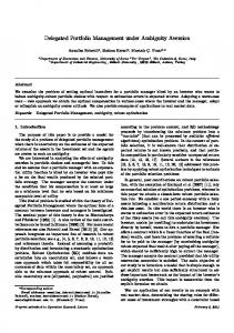
There have been two previous imaging experiments on ambiguity aversion, both with PET— Smith et al. [63], and Rusticini [51] et al.. Given the small number of imaging studies using economic tasks, this is somewhat surprising. I will review these closely. Smith et al. [63] was the first imaging study to investigate difference in brain activity under ambiguity and risk. Their study serves as an excellent road map for our study, as it illustrates a number of challenges and pitfalls. This study used the traditional Ellsberg paradigm. Subjects chose between two urns in each of two conditions—risk and ambiguity. In the risk condition, subjects chose between two urns with known composition of red, blue, and yellow balls. In the ambiguous condition, subjects also chose between two urns. In the first urn, one of the colors was in a known proportion, the remaining two in unknown proportion. The second urn was a risky urn of known composition, similar to those in the risky condition. Thus, the only difference in screen is the very minimal visual change from a risky to ambiguous urn. The conditions were further separated into a high and low payoff condition. Figure 1 shows a sample screen from the experiment. Gambles were not played after the subjects made their choice. Instead, after 9

Subliminal priming is commonly achieved by a task called backward masking. In this task, the subject is exposed to two stimuli. Stimuli A appears on a screen briefly, e.g., 30ms, and is immediately followed by stimuli B, which appear for say, 400ms. Subjects will not have any explicit knowledge of ever seeing stimuli A (and will identify it out of a sample of A and a group of novel stimuli at chance). Subjects will exhibit, however, increased GSR at the time of stimuli delivery if stimuli A is, for example, a fearful face or some other negative stimuli. Recent imaging experiments have confirmed that the amygdala is activated in such a task. 10 The insula is a part of the somatosensory cortex. Most of the somatosensory cortex has representation of touch throughout the human body. The insula, however, has representations of internal states. This places the FI in an ideal place to integrate signals from higher cortical levels and those from lower subcortical structures.

9

Figure 1: Sample screen used in Smith et al. study. (From their paper).

subjects finished the scanning, one of the gambles was chosen at random, and the gamble was resolved. The rationale for this is to eliminate learning as well any income effects that might be introduced. The activations found in Smith et al. include orbitofrontal, inferior frontal gyrus, lateral parietal, and a host of other areas. The main drawback to their study is the overwhelming amount of activation seen in their data analysis. This suggests that the design failed to control for the differences in risk and ambiguity. There are a number of candidate hypotheses 1. Choosing between gambles: subjects in the Smith et al. study are choosing between two quite complicated gambles. Note that although there is minimal difference between the risk and ambiguous condition, there is a lot of numerical information to process. These are quite difficult tasks to perform. 2. Ambiguous condition contains risk as well: their comparison conditions are inappropriate. In the risky condition, subjects are presented with 2 urns of known composition. In the ambiguity case, subjects are presented with an urn of unknown composition and an urn of known composition. Suppose processing for risk and ambiguous probabilities were to occur in different neural structures, the ambiguous condition would then activate both the risk and ambiguous structures. 3. PET: the low temporal and spatial resolution of PET introduced unknown complications. In addition, there may be a selection bias in the subject pool given the use of PET, as it requires the subject to be internally administered a radioactive element. In spite of the overabundance of activations, their results is also illustrative of the areas that we can expect to see. As will be shown later, the activity in Smith et al. was a strict subset of the present study. In particular, they found highly significant activity in the orbitofrontal cortex, the dorsolateral prefrontal, intraparietal area. The activation in the study also included a subcortical activation which was labeled entorhinal cortex but which may be the amygdala. It also looks very close to the activity seen in the present study. In summary, Smith et al. gives us a good guide into the pitfalls of a traditional Ellsberg paradox experiment. First, choices that look simple are actually quite difficult, requiring the brain to recruit a number of areas that are perhaps unrelated to ambiguity per se. These 10

areas are difficult to control for and subtract out, given that they are included in both risky and ambiguous conditions. Making the task simple and tractable for subjects therefore, will be crucial. Absence of such controls is potentially disastrous. For example Smith et al. was not to make any statements about potential brain areas underlying decision making under ambiguity. Rusticini et al. [51] is an ambitious study that tries to tie together choice, response times, and brain activation, using certain (CR), ambiguous (AR), risky (RR), and partially– ambiguous (PAR) gambles11 . They used a similar paradigm as Smith et al. Subjects were presented with two lotteries to choose from. Unlike Smith et al., however, there is a “main lottery”—of any of the certain, ambiguous, risky, or partially ambiguous gambles, and a “reference” lottery—of either certain or risky gambles. This study thus had a number of conditions, each of which differ slightly in their presentation. The most surprising finding in the Rusticini is the absence of activity in the entire prefrontal cortex. Of the contrasts conducted, only RR − P AR yielded limited evidence of OFC. This is extremely surprising given the strong OFC activity seen in Smith et al. (and, as will be discussed, in the present study), as well as the strong theoretic reasons of why OFC should be involved in such tasks. The stimuli used in [51] do not seem to be radically different than the ones used in [63], both involved choices between ambiguity and risk, with the former including an extra condition of the partially ambiguous case. Details about specific subtractions, as well as pictures of activations are scant in the paper, as it is still in working paper form. However, the existence of occipital activity in the study suggests that very basic perception and visual stimuli are not being controlled. In light of these results, the authors hypothesized that the difference is due to the task involved, which is one of choice, as opposed to one of learning and choice. In short, the authors argue that it is learning that is critical in activating the OFC. This runs counter to our knowledge that the delivery and anticipation of primary reinforcers (including money, which may or may not be a primary reinforcer) is sufficient to activate the OFC. This has been demonstrated in neuroimaging experiments on humans [?] and at the cellular level in monkeys [50]. In addition, their experimental procedure is identical to that of Smith et al., in that gambles are not resolved during the course of the scanning. Only at the end of the experiment is one of the gambles chosen and played. Another hypothesis is that the proliferation of conditions in the study increased the variance of the results (for example, all screens containing an ambiguous gamble is classified as part of the ambiguous condition), and decreased the sensitivity and efficiency of the estimates. Regardless, the results of this study is puzzling indeed. 11

Partially ambiguous gambles are ones where the subject is told that the urn contains at least a certain proportion of balls.

11

6

Experiment Design

Each treatment consists of two conditions, with 24 choices in each condition. The stimuli are presented in a blocked fashion of 4 choices in each block, in an ABAB design. Ellsberg Type Gambles In light of the results from Smith et al. and Rusticini et al., we strived to present stimuli that are easy to calculate and which do not intersect each other. The table below shows screenshots from the 2 colored problem. Subjects choose between urns with red and blue balls, and a certain payoff. Like Smith et al., the difference between the risky and ambiguous screens are minimal. In our case, however, the calculations necessary for calculating payoffs is substantially simplified.

Ambiguity.

Risk

Table 1: Ellsberg condition. The screens are presented side-by-side for comparison purposes. The subject sees one screen at a time. For each screen, the right box shows the gamble, where the top number shows of total cards in deck, the bottom number shows gamble payoff. The left box shows sure payoff. Note that the current setup has a slight difference the standard Ellsberg problem, which does not include a degenerate gamble (the certain payoff). This should not change subject’s attitude to ambiguity, however. Indeed, that the partial ordering of bets should remain unchanged when a mixture is introduced with a constant act is one of the axioms introduced by Gilboa and Schmeidler when weakening the independence axiom. Knowledge Type Gambles In most studies of Ellsberg’s paradox, researchers have used some variations on the Ellsberg urns. The problem with this approach in the scanner is that the very nature of the problem leads subjects to perform some sort of calculation, whether expected value calculations or not. This confounds effects of the ambiguity-risk treatment versus one where the effects are artifacts of different computational processes used in the risk and ambiguity treatments. This is especially a worry with intraparietal activity, as it may reflect expected reward assessments, as posited by Glimcher [46], or something else. 12


 

Low Ambiguity

High Ambiguity

Table 2: Right hand side box contains the question. Subjects can choose yes or no to the questions. Below the acts is the payoff. Left hand side contains the sure payoff. This limits the number of hypotheses we are able to distinguish. It will not, for example, limit the identification of the Gilboa-Schmeidler hypothesis, or indeed any hypothesis that posits a difference in the measurement of risk and ambiguity. For example, if the algorithm that people use to represent ambiguity is a Choquet integral, this should show up in the subtraction between risk and ambiguity, up to the sensitivity of the scanner. If on the other hand, however, ambiguity is distinguished between risk by the addition of another system, e.g., fear or paranoia, at the lack of an algorithm that can be used to weight the probabilities and payoffs, then what we’re studying in the contrasts is fundamentally different from ambiguity.12 Betting Against Informed Opponent As noted in the introduction, a common view about ambiguity aversion is that subjects are “confused” when making their choices in the laboratory. This interpretation is similar to the hypothesis that subjects act in finite horizon games, specifically, one-shot games, as they would in a repeated game. The intuition behind this view is roughly that “life is a repeated game.” People therefore behave in these “artificial” laboratory sessions as if they are playing in a infinitely repeated game. Perhaps as a clue, Chow and Sarin [12] distinguished between “known”, “unknown,” and “unknowable” probabilities. They find that subjects’ behavior in the “unknowable” probabilities fall somewhere between that of known and unknown probabilities. This account is consistent with the view that agents are suspicious that they might be playing against an opponent, e.g., the experimenter, that is hostile and has more information. 12 Using real world questions may also have an advantage in the behavioral aspect. Fox and Tversky found that, compared to pricing gambles on urns, pricing real world situations with familiar and unfamiliar events—e.g., temperature of Istanbul versus that of San Francisco—pricing on real world events yielded a higher ambiguity premium [20]. The robustness of the effect is not known.

13

0

Informed Opponent

Uninformed Opponent

Table 3: Top text gives the number of cards opponent will draw. The rest is identical to the risk condition in the Ellsberg treatment. This argument suffers from the stylized fact that, when faced with an ambiguous event, ambiguity averse individuals will neither bet on the event nor its complement. In this case, the expected payoff to the partially informed agent is 0, assuming that the subject is randomizing. In this sense it is quite similar to the argument concerning the inability of people to not play the dominant strategy in a one-shot game. The argument is that people are “used to” playing that particular strategy that is not adaptive in this instance. There is a tricky design issue of how to implement betting against an informed opponent (BAIO). One way is just to have them choose between cash and a BAIO gamble– if they choose the gamble, they only play if the opponent chooses a different color. This can be remedied by having a control condition where choices are randomized. I.e., players play against a number generator which generates choices randomly. Subliminal Priming This condition is really a separate, follow-up experiment to the previous. As it is still extremely preliminary, however, I will present it as a fourth treatment in this array of experiments. As discussed in the introduction, the amygdala and other structures involved in emotion are activated in subliminal priming experiments, even as the stimuli is not seen consciously. There is some evidence that these primes can in fact influence behavior, albeit in an ephemeral manner [67]. Table 4 Relatively few studies have directly tried to manipulate emotions in decision making tasks. Part of the problem lies in the ethicality of such studies. Hertel et al. studied a 4 player public goods game where mood is manipulated through the viewing of either a happy or sad film clip [28]. In addition, subjects’ beliefs were manipulated by telling the subjects’ different baseline rates, either that “most people contributed” or “most people kept.” They found that subjects who were shown a happy film tend to act in accordance to the rates given, whereas subjects who viewed the sad film defected more. They interpreted this finding as supporting the idea that individuals tend to hold firmer beliefs when they 14

Table 4: Sample Face Stimuli are happy, whereas they are more willing to explore when fearful or sad. In a similar study, Johnson and Tversky manipulated affect by having subjects read a brief newspaper report of a tragic event. [29] They found that such a report increased the probability assessment of negative events globally. An account of a happy event also produced a global decrease in the judged frequency of risk. In this condition, all trials consists of risky gambles. The gambles are separated as Happy or Angry, depending on the type of face preceding it. Payoffs in the Happy condition is a linear transformation of those in the Angry condition. This allows us to test whether the addition of fear in a risky decision is equivalent to that of ambiguity decision. Table 4 shows a sample of the faces used in the experiment. Before each gamble, the subject is presented with a cross for 30 ms, immediately followed by the subliminal stimulus (either happy or angry face) for 16 ms, and then by a neutral face for 400 ms. The subject has to correctly identify the gender of the neutral face (as the subliminal stimulus is not consciously perceived, they only see the neutral face). Following a correct face identification, the subject is presented with a gamble.

6.1

Protocol

Imaging Data Acquisition Scanning was performed using a Siemens Magnetom system (Ehrlangen, Germany) at 3 Tesla to acquire gradient-echo, echo-planar T2* weighted images with BOLD (blood oxygenation-dependent) contrast. For each subject, 32 − 34 slices, depending on brain volume, with 3.25 mm in slice thickness was acquired (TR = 2000 ms, TE = 2 ms, flip angle = 90, 64 × 64 matrix). Data were analyzed using SPM2 (Wellcome Department of Cognitive Neurology, London, UK). Functional scans were first corrected for slice timing correction via linear interpolation. This accounts for the time between the first slice taken of the brain and the last slice, i.e., the signal from each slice is aligned to a common time point, in this case the middle slice. Motion correction of images, for head movement during the course of a scanning session, was performed using a 6-parameter rigid-body transformation [22]. Images were then spatially normalized to the Montreal Neurological Institute (MNI) template by applying a 12 parameter affine transformation followed by nonlinear warping using basis functions [2]. This procedure standardizes all subjects to a common atlas, to allow between-subject 15

neuroanatomical comparability. Finally, images were smoothed with a Gaussian kernel of 8 mm FWHM. Behavioral Data Acquisition Subjects were presented with the decision task while laying in the scanner. Stimuli were delivered with goggles connected to a computer via fiber optic cables. Subjects made their decisions by pressing buttons on button boxes that they held in their hands. Data Analysis Data analysis was performed on SPM2, via a two-step random-effects statistical analysis procedure. First, the dependent variable (the MR signal) is scaled using proportional scaling, to control for global differences. Low frequency noise13 was removed by temporally filtering the data with a low pass filter. A separate linear model yt = α + βamb Λ (damb ) + βrisk Λ (drisk ) + βpost Λ (dpost ) + δyt−1 + εt . was specified for each subject, where damb , drisk , and dpost are the dummies for the conditions ambiguity, risk, and post−decision, respectively, and Λ is the convolution operator—a canonical hemodynamic response function (HRF) consisting of a 3rd order gamma function. This idealized HRF serves as an approximation of the hemodynamic response. Autocorrelation of the hemodynamic responses is modeled as a AR(1) process. Parameters are estimates using a ReML procedure. Post-hoc contrasts were performed on the coefficients, voxel–by–voxel. For the ambiguity > risk condition, a t-test of βˆamb > βˆrisk was performed to find areas that are significantly activated in the ambiguity trials relative to the risk trials, and similarly for βˆrisk > βˆamb 14 . A second level analysis is performed on the contrast maps from the first stage. I assume that the estimates βˆamb and βˆrisk are sampled independently between subjects. This is a reasonable assumption given this is a decision task that does not involve interaction between i subjects. A t-test was performed on the estimates βˆamb derived from the first level GLM.

7 7.1

Results Ellsberg Urn

Table 5 shows glass brain of areas activated in the Ellsberg condition. Notably, there is posterior cingulate (PCC), inferior parietal lobule (IPL), frontoinsular cortex (FI), premotor cortex, and orbitofrontal cortex (OFC) in the Ambiguity > Risk contrast. The Risk > Ambiguity contrast revealed ventral striatum (VS), and superior temporal lobe. Table 6 shows the sectional views. 13

The responses of interest are generally of high frequency. On the other hand various noises, from breathing to heart-rate to drifts in the scanner, are of low frequency. 14 This corresponds to a contrast matrix of [1, −1, 0] for βˆamb > βˆrisk , and [−1, 1, 0] for βˆrisk > βˆamb .

16

Ambiguity > Risk : p = 0.005, k = 4

Risk > Ambiguity, p = 0.0005, k=4

Table 5: Ellsberg condition

7.2

World Knowledge Condition

The world knowledge condition (Table 7) revealed a different set of activations from the Ellsberg urn. The Ambiguity > Risk contrast revealed temporo-parietal junction, motor cortex, FI, and dorsolateral prefrontal cortex. The Risk > Ambiguity contrast revealed ventral striatum (VS), PCC, and premotor cortex. It is interesting to note that the location of the PCC flipped from the Ambiguity > Risk contrast to Risk > Ambiguity.Table 12 shows the sectional views.

7.3

Ellsberg Urn + World Knowledge Questions

Although we strived to control as carefully as possible any nuisance parameters, there are clearly variables that we are not able to control adequately, as they are part of the design. For example, in the world knowledge questions “Muhammed Ali won his first title after the 8th round” and “Hal Bagwell holds the boxing record for most consecutive wins without a loss”, there is clearly much more difference than simply the “ambiguity” of the question15 . Likewise for the Ellsberg condition. Pooling the results allows us to find the common features of the two conditions. An objection to pooling the time series is that there is potentially two different data generating processes here. For example, let bji be the estimated parameter b for subject i in condition j. If b1 is much larger than 0, but b2 = 0, our estimate ˆb could be greater than 0. This is further complicated by the fact that this also depends on the region in question. Suppose the hippocampus is involved in the Ellsberg condition but not in the RW K condition, but that the orbitofrontal cortex is in both, then it might be the case the data from the 15

Part of this is resolved by mixing questions from different knowledge domains (see appendix).

17

hippocampus cannot be pooled where those from the OFC can. One approach is to first test whether the data from the two sessions could be pooled, and then perform a second level analysis only on those voxels that survive the first test. That approach has its own problems [25]. Below I present two approaches. One by pooling all of the data from the two conditions, and treating all observations as independent. The second method makes the minimal assumptions on the underlying data generating process by taking the intersection of the activations from the two conditions. 7.3.1

Pooled Analysis

Figure 9 shows results from pooling the contrast maps from the Ellsberg and the RW K conditions. 7.3.2

Conjuction Map

Table 10 presents the intersection of the activation maps from the two conditions—Ellsberg and RW K. As opposed to the pooled analysis, only two structure, one in each contrast, is found in the intersection—Right FI in the Ambiguity > Risk contrast, and bilateral ventral striatum for Risk > Ambiguity. This suggests that there is, not surprisingly, structural changes in the way the brain processes ambiguity.

7.4

Betting Against Informed Opponents

Table 11 presents the activation in the BAIO treatment. Interestingly, BAIO also shows activity in the FI region in the Ambiguity > Risk contrast. It does not however, show the ventral striatum activity in the Risk > Amiguity treatment.

7.5

Subliminal Priming

It is still too early in the subliminal priming treatment to present group results. Here I present results from one subject showing that the subliminal priming condition does indeed leave behind the neural activations that we expect. Table 13 shows that in the Angry > Happy contrast, only the amygdala is activated. In the Happy > Angry contrast, the orbitofrontal is activated. Whether this translates into an effect in the decision making stage awaits more data.

8

Discussion

Utility Based Models These results support the utility-based models of ambiguity aversion. In addition to behavioral changes, Bechara et al. also found that OFC patients do not exhibit normal GSR [4]. Normal subjects display heightened GSR [65] during later trials when choosing the high risk deck, upon which they cease to choose the high risk deck. OFC 18

patients on the other hand keep choosing from the high risk deck, and do not exhibit heightened GSR. This appears to be a global level effect, as these patients also have abnormally low responses to disturbing or exciting images [?]16 . Because of the extent of damage in a number of the patients, it is difficult to ascertain which substructure in the OFC is responsible for the behavioral changes. Neuroimaging and psychophysiological studies have given some clues to this. In a study that combined GSR and fMRI while subjects performed a probability matching experiment, Critchley et al. found that GSR responses correlated with activity in areas which included the FI [14] [15]. In a similar study but using the gambling task, Patterson et al. also found that GSR correlated with activity near OFC/Insula [44]. Elliot et al. found activity in FI correlated with winning and losing streaks17 [17]. FI areas in this study overlaps with those found in imaging study on the ultimatum game by Sanfey et al. [52]. They found that activity in that region was correlated with rejection of unfair offers. In a particularly careful study, Rogers et al. [47] tested OFC patients, other prefrontal lesion patient, amphetamine abusers18 , normal subjects given a drug simulating the effects of amphetamine19 , and normal controls. They used a variation of the gambling task with a known probability distribution. There was also a bet during each trial that the subject could take, allowing the experimenter to assess the risk attitudes of the subjects. They found that card choices of OFC patients, amphetamine patients, and normals with lowered plasma tryptophan were similar. Even though the probability distribution is known, these subjects chose the color with the lower probability (a dominated choice) significantly more frequently than normal controls. OFC lesion patients, however, do not appear to be more risk averse; when allowed to wager on the outcome, lesion patients wagered significantly higher amounts than did normal controls. This, combined with studies showing that OFC patients perform normally in probability matching tasks [37], suggest that the difference between OFC patients, amphetamine abusers, and normal controls is one of differences in utility evaluations, not probability. Probability-Based Models Despite this, there is some support for the probability-based models. There is clear evidence that there is LIP activity in Ambiguity > Risk in the Ellsberg condition. This coincides with Platt and Glimcher’s work on expected utility neurons in the monkey LIP [46]. This could be interpreted as evidence that subjects are evaluating probabilities differently than they do in the risk condition. To the extent that the two conditions both conditions reflect decision-making under ambiguity, the absence of LIP activation in the RW K condition, however, suggests that the 16

Preliminary results from Camerer and Adolphs show that OFC patients do not exhibit ambiguity aversion. 17 Interestingly, they found that this area is activated by both winning and losing streaks. However, this is consistent with the finding of heightened GSR measure during winning and losing streaks (NEED CITE). 18 Amphetamine is known to affect the dopaminergic system. 19 This is done by temporarily lowering central 5-hydroxytryptamine (5-HT) activity (to simulate effects of amphetamine use)

19

probability-based models do not carry across domains. In fact, it is difficult to imagine how a probability-based algorithm would be implemented in the world knowledge condition. Assuming that the view that ventral striatum is involved in probability evaluation and learning is the correct one, results from the Risk > Ambiguity contrast also suggest that there is some difference in probability evaluation under ambiguity. It is difficult to see, however, how existing models of ambiguity aversion fits with these result, as in all or almost all probability-based models, decision weights are modifications of probability that are more complicated to compute than probabilities. This is especially true of Schmeidler’s subadditive probabilities. This does not, however, preclude the possibility that the algorithms actually employed by the brain may be an approximation of the models, which would almost certainly be case. Taken together, these results suggest that, although subjects may evaluate probabilities differently in the face of ambiguity, it is not a necessary component to the behavioral effects of ambiguity aversion, whereas a state-dependent utility appear to be necessary. Adversarial Nature/Experimenter The FI activation also suggest that there is some validity to the idea that opponents face an ambiguous decision as they do an adversarial opponent. The absence of ventral striatum activity, however, shows that this is not the whole picture. In fact, this supports the view that subjects process probability differently in the ambiguity and risk conditions, as in the BAIO condition, probability distribution of the decks are all explicit. Conclusion There are two basic implications from the current study about how the brain makes decisions under uncertainty with known or well-informed odds, and ambiguous gambles where there is missing information about card decks or low knowledge about natural events. The first implication is that a na¨ıve view often expressed in decision theory—that the weight of evidence should not matter, holding the implications of that evidence constant—is wrong. The brains approaches decision making under risk and ambiguity differently. The second implication is that emotional regions, especially the important area FI implicated in processing of disgust, pain, and other negative discomforts, are differentially active in evaluating ambiguous gambles. This activation is supportive of the view that people are pessimistic about ambiguous gambles, or weight their utility lower, provided the neural mechanism for those adjustments are located in FI. At the same time, there is stronger activation in striatum when facing known-risk and high-knowledge gambles, an area known to be activated by a wide range of rewards. This implies that evaluating risky gambles is somehow more basically rewarding. Further research will help us understand more about these regions of differential activation.

References [1] Anscombe, Francis and Robert Aumann. 1963. “A Definition of Subjective Probability.” Annals of Mathematics 34: 199-205. 20

[2] Ashburner, J. and Karl Friston. 1999. “Nonlinear Spatial Normalization Using Basis Functions.” Human Brain Mapping 7: 254-266. [3] Bechara, Antoine, Hanna Damasio and Antonnio Damasio. 2000. “Emotion, decision making and the orbitofrontal cortex.” Cerebral Cortex 10: 295-307. [4] Bechara, Antoine, Daniel Tranel, Hanna Damasio, and Antonio Damasio. 1996. “Failure to respond autonomically to anticipated future outcomes following damage to prefrontal cortex.” Cerebral Cortex 6: 215-225. [5] Becker, Selwyn and Fred Brownson. 1964. “What Price Ambiguity? On the Role of Ambiguity in Decision Making.” Journal of Political Economy 72: 62-73. [6] Berridge, Kent, and Piotr Winkielman. 2003. “What is an unconscious emotion? (The case for unconscious “liking”)” Cognition and Emotion 17, 181-211. [7] Berns, G.S. 2001. “Predictability Modulates Human Brain REsponse to Reward.” Journal of Neuroscience 21: 2793-2798. [8] Bossaerts, Peter. 2003. “The physiological foundations for the theory of financial decision making.” Unpublished manuscript. [9] Bossaerts, Peter, Paolo Ghirardato, and William Zame. 2003. “The Impact of Ambiguity on Prices and Allocations in Competitive Financial Markets.” Caltech working paper. [10] Camerer, Colin, and Martin Weber. 1992. “Recent developments in modeling preferences: Uncertainty and ambiguity.” Journal of Risk and Uncertainty, 5: 325-370. [11] Camerer, Colin and Howard Kunreuther. 1989. “Experimental Markets for Insurance.” Journal of Risk and Uncertainty 2: 265-300. [12] Chow, Clare Chua and Rakesh Sarin. “Known, Unknown, and Unknowable Uncertainties.” Working paper. [13] Cohen, Mark and Susan Bookheimer. 1994. “Localization of Brain Function with Magnetic Resonance Imaging.” Trends in Neurosciences Vol 17. [14] Critchley, Hugo, Rebecca Elliot, Christopher Mathias, and Raymond Dolan. 2000. “Neural Activity Relating to Generation and Representation of Galvanic Skin Conductance Responses: A Functional Magnetic Resonance Imaging Study.” Journal of Neuroscience 20, 3033-3040. [15] Critchley, Hugo, Christopher Mathias and Raymond Dolan. 2001. “Neural Activity in the Human Brain Relating to Uncertanty and Arousal during Anticipation.” Neuron 29: 537-545. [16] Dow, James and Sergio Ribeiro da Costa Werlang. 1991. “Uncertainty Aversion, Risk Aversion, and the Optimal Choice of Portfolio.” Econometrica LX: 197-204. 21

[17] Elliott, Rebecca, Karl Friston, and Raymond Dolan. 2000. “Dissociable neural responses in human reward systems.” Journal of Neuroscience 20, 6159-6165. [18] Epstein, Larry and Tan Wang. 1994. “Intertemporal Asset-Pricing Under Knightian Uncertainty.” Econometrica LXII: 283-322. [19] the naomi eisenberger et al 9last author is Matthew Lieberman, ucla) study in science on social exclusion shows some insula activation (not graphically shown but in text). this is useful for us on ambig, so make a note. [20] Fox, Craig and Amos Tversky. “Ambiguity Aversion and Comparative Ignorance.” Quarterly Journal of Economics 110: 585-603. [21] Franke, G¨ unter. 1978. “Expected Utility with Ambiguous Probabilities and ‘Irrational Parameters’.” Theory and Decision 9: 267-287. [22] Friston, Karl, J. Ashburner, C Frith, Jean-Bapiste Poline, J Heather, and R Frakowiak. 1995a. “Spatial Registration and Normalization of Images.” Human Brain Mapping 2: 1-25. [23] Friston, Karl, C Frith, R Frackowiak, and R Turner. 1995b. “Characterizing Dynamic Brain Responses with fMRI: A Multivariate Approach.” NeuroImage 2: 166-172. [24] Gilboa, Itzhak, and David Schmeidler. 1989. “Maxmin expected utility with non-unique prior.” Journal of Mathematical Economics 18, 141-153. [25] Greene. 2000. Econometric Analysis. Prentice-Hall: New Jersey. [26] Hansen, Lars Peter and Thomas Sargent. 2001. “Robust Control and Model Uncertainty.” American Economic Review 91: 60-66. [27] Harlow, JM. 1968. Recovery of the passage of an iron bar through the head. Pub Mass Med Soc 2: 327-347. [28] Hertel, Guido, Jochen Neuhof, Thomas Theuer and Norbert Kerr. 2000. “Mood effects on cooperation in small groups: Does positive mood simply lead to more cooperation.” Cognition and Emotion 14: 441-472. [29] Johnson, Eric and Amos Tversky. 1983. “Affect, Generalization, and the Perception of Risk.” Journal of Personality and Social Psychology 45: 20-31. [30] Joseph, Michael, Krishna Dutla, and Andrew Young. 2003. “The Interpretation of the Measurement of Nucleas Accumbens Dopamine by In Vivo Dialysis: The Kick, The Craving, Or The Cognition?” Neuroscience and Biobehavioral Reviews 27: 527-541. [31] Kahneman, Daniel, and Amos Tversky. 1979. “Prospect theory: An analysis of decision under risk.” Econometrica, 47, 264-291. 22

[32] Kahn, Itamar, Yehezkel Yshurun, Pia Rotshtein, Itzhak Fried, Dafna Ben-Bashat, and Talma Hendler. 2002. “The role of the amygdala in signaling prospective outcome of choice.” Neuron 33: 983-994. [33] Keynes, John Maynard. 1921. A Treatise on Probability. London: MacMillan. [34] Knight, Frank. 1921. Risk, Uncertainty, and Profit. Boston: Houghton Mifflin. [35] Knutson, Brian. 2001. ‘Dissociation of Reward Anticipation and Outcome with EventRelated fMRI.” NeuroReport 12, 3683-3687. [36] MacCrimmon, Kenneth. 1968. “Descriptive and Normative Implications of the DecisionTheory Postulates.” In K. Borch and J. Mossin (eds.), Risk and Uncertainty. London: MacMillan. [37] Manes, Facundo, Barbara Sahakian, Luke Clark, Robert Rogers, Nagui Antoun, Mike Aitken, and Trevor Robbins. 2002. “Decision-making processes following damage to the prefrontal cortex.” Brain: 125, 624-639. [38] Matsumoto, D., and P. Ekman. 1988. “Japanese and Caucasian Facial Expressions of Emotion (JACFEE) and Neutral Faces (JACNeuF). Report availabe from Intercultural and Emotion Research Laboratory, Department of Psychology, San Francisco State University. [39] Montague, P. Read and Gregory Berns. 2002. “Neural Economics and the Biological Substrates of Valuation.” Neuron 36: 265–284. [40] Nauta, EJ. 1990. “The problem of the frontal lobe: a reinterpretation.” Journal of Psychiatric Research 8:167-187. [41] O’Doherty, J., Kringelbach, M., Rolls, E. T., Hornak, J. and Andrews, C., (2001), “Abstract reward and punishment representations in the human orbito frontal cortex”, Nature Neuroscience, 4, 1, 95-102 [42] O’Doherty, John. “Can’t Learn Without You.” Nature. ¨ ur, D. and J.L. Price. 2000. “The Organization of Networks within the Orbital and [43] Ong¨ Medial Prefrontal Cortex of Rats, Monkeys and Humans.” Cerebral Cortex 10: 206-219. [44] Patterson, James, Leslie Ungerleider, and Peter Bandettini. 2002. Task-Independent Functional Brain Activity Correlation with Skin Conductance Changes: An fMRI Study. NeuroImage 17 1797-1806. [45] Phelps, Edmund S., ”The New Microeconomics in Employment and Inflation Theory,” in Microeconomic Foundations of Employment and Inflation Theory. New York: Norton, 1970, pp. 1-23.

23

[46] Platt, Michael and Paul Glimcher. 1999. “Neural correlates of decision variables in parietal cortex.” Nature 400: 233-238. [47] Rogers, R.D., B. J. Everitt, A. Baldacchino, A. J. Blackshaw, R. Swainson, K. Wynne, N. B. Baker, J. Hunter, T. Carthy, E. Booker, M. London, J. F. W. Deakin, B. J. Sahakian, and T. W. Robbins. 1999. “Dissociable Deficits in the Decision-Making Cognition of Chronic Amphetamine Abusers, Opiate Abusers, Patients with Focal Damage to Prefrontal Cortex, and Tryptophan-Depleted Normal Volunteers: Evidence for Monoaminergic Mechanisms” Neuropsychopharmacology 20: 322-339 [48] Ronen, J. 1971. “Some effects of sequential aggregation in accounting and decisionmaking.” Journal of Accounting Research, 77, 326-336. [49] Rolls ET. The orbitofrontal cortex and reward. Cereb Cortex 2000; 20:284–94. [50] Rolls ET. The neural basis of emotion. In: Rolls ET, editor. The brain and emotion. New York: Oxford University Press; 1999. p. 112–37. [51] Rusticini, Aldo, John Dickhaut, Paolo Ghirardato, Kip Smith, and Jos´e V. Pardo. A Brain Imaging Study of the Choice Procedure. Working paper, 2003. [52] Sanfey, Alan, James Rilling, Jessica Aronson, Leigh Nystrom, and Jonathan Cohen. 2003. “The neural basis of economic decision-making in the ultimatum game.” Science 300, 1755-1758. [53] Sarin, Rakesh and Martin Weber. 1989. “The Effect of Ambiguity in Market Setting.” Management Science 39: 135-149. [54] Sarin, Rakesh and Robert Winkler. 1992. “Ambiguity and Decision Modeling: A Preference-Based Approach.” Journal of Risk and Uncertainty 5: 389-407. [55] Schoenbaum, Geoffrey, Barry Setlow, Michael Saddoris and Michela Gallagher. 2003. “Encoding Predicted Outcome and Acquired Value in Orbitfrontal Cortex during Cue Sampling Depends upon Input from Basolateral Amygdala.” Neuron 39: 855-867. [56] Schwartz, Norbert. 2000. “Emotion, cognition, and decision making.” 14: 433-440. [57] Schmeidler, David. 1989. ”Subjective probability and expected utility without additivity”, Econometrica 57, 571-587. [58] Shultz, Wolfram. “Predictive Reward Signal of Dopamine Neurons.” Journal of Neurophysiology. [59] Shultz, Wolfram. 2001. “Reward Signaling by Dopamine Neurons.” The Neuroscientist 7: 293-302. [60] Shultz, Wolfram, L´eon Tremblay and Jeffrey Hollerman. 2000. Reward Processing in Primate Orbitofrontal and Basal Ganglia. Cerebral Cortex 10: 272-283. 24

[61] Segal, Uzi. 1987. “The Ellsberg paradox and risk aversion: an anticipated utility approach.” International Economic Review 28, 175-201. [62] Slovic, Paul and Amos Tversky. 1974. “Who accepts Savage’s axiom?” Behavioral Science 19, 368-373. [63] Smith, Kip, John Dickhaut, Kevin McCabe, and Jos´e V. Pardo. 2002. “Neuronal Substrates for Choice Under Ambiguity, Risk, Gains, and Losses.” Management Science 48: 711-718. [64] Smith, Vernon. 1969. “Measuring Nonmonetary Utilities in Uncertain Choices: The Ellsberg Urn.” Quarterly Journal of Economics 83: 325-329. [65] Tranel, Daniel, and Hanna Damasio. “Neuroanatomical correlates of electrodermal skin conductance responses.” Psychophysiology 31, 427-438. [66] Wald, Abraham, 1950. Statistical decision functions. Wiley, New York. [67] Winkielman, Piotr, Kent C. Berridge and Julia Wilbarger. “Unconscious affective reactions to masked happy versus angry faces influence consumption behavior and judgments of value.” Personality and Social Psychology Bulletin, in press.

A

Methods in Neuroscience

Because of the results presented in the following section include various methods that the reader may not be familiar with, I will give a brief overview of the various techniques. Figure 2 shows the spatial/temporal resolution of the various methods, as well as their invasiveness. Functional Magnetic Resonance Imaging (fMRI) fMRI takes advantage of the fact that the brain is composed mostly of water. The magnetic field induces the protons in the hydrogen molecules to align, Crudely speaking, a transitory increase in blood volume takes place in activated areas of the brain. In particular, oxygen content of venous blood increases during brain activation, resulting in increased MR signal intensity. fMRI takes advantage of the difference between oxygenated and deoxygenated blood as an endogenous contrast agent [13]. Spatial and Temporal Resolution The spatial resolution of fMRI can feasibly be brought to the µm level. Unfortunately there is a trade-off between the spatial resolution and noise, and thus, temporal resolution. This remains an area of active research. For all practical purposes, the spatial resolution of the images are limited to 2-3 mm3 , whereas temporal resolution at 2-3 seconds. [13]

25

Figure 2: Plot of the temporal (x-axis), spatial resolution (y-axis), and invasiveness (temperature) of method. (MEG = magneto-encephalography; ERP = evoked response potentials; fMRI = functional magnetic resonance imaging; PET = positron emission tomography.)

Data analysis is an active area of research, as there are a number of technical issues that are yet to be adequately resolved. Standard time series models and panels in general do not include spatial correlation. This is especially important in the brain due to the extensive connections between different parts of the brain. Currently, however, fMRI data is most frequently analyzed using standard linear regression models where the error term is modeled as an AR(n)20 process. The coefficients are then compared using t-tests21 . Significance levels is a particularly active area of research. Because in a single scan there is often hundreds of thousand voxels, there is an enormous multiple comparison problem. Standard correction processes, however, tend to be too stringent as it overestimates the false-positive rates of activity. There has been work to extend a Bayesian framework into fMRI data analysis, although that is still not widely used. Displaying activations There are a number of methods to display brain activations, complicated by their 3D nature. Two are used in this paper. One such is the so called “glass” brain, so called because it projects the 3-dimensional brain down to three different 2-dimensional views, as if one were looking at a glass brain. The other is the “sectional view.” This view displays the three orthogonal planes centered at any one point in the brain. 20 21

Almost exclusively AR(1). This is what is commonly called “cognitive subtraction.”

26

The three planes are respectively: The “coronal view”, that runs from the front to the back of the brain; the “sagittal view”, from left to right; and the “axial view”, from top down.

Sectional view

Glass brain

Positronic Emission Tomography (PET) Under PET, subjects are either injected or consume radioactive dye with a certain half life, whose positronic emission the scanner records. PET has poor temporal and spatial resolution than fMRI. Because subjects are injected with radioactivity dyes, however, it does have the advantage of being more sensitive in certain domains, such as being able to track neurotransmitters. PET data is analyzed much the same way fMRI data is. Because of the poorer spatial and temporal resolution, however, some of the issues in fMRI data analysis is not present in PET. Cell Recordings Whereas fMRI and PET are commonly used with human subjects, single cell recordings are almost exclusively performed on animals, especially rats and nonhuman primates. Electrodes are implanted in the brain and record neuronal firing. The temporal resolution of the single and multiple cell recordings therefore is on the order of 1 − 3µm and spatial resolution is at the single neuron level. Lesions Damage or ablation of the brain has proven useful in understanding the functions of the brain over the years. Lesions provide a direct path to testing the causes of behavior. In humans, however, this is limited to accidents. Lesions are also limited in the fact that the lesioned brain is by a fortiori abnormal. Generalization to the normal brain functions is always questionable without corroborating evidence from other methods.

27

B

Experiment Design

B.1

BAIO

Example 7 Suppose that the gamble consists of an urn of N balls, K of which are red, the rest are green. The agent bets against an informed agent who has partial information about the contents of the urn. That is, let the informed agent draw n balls from the urn. To simplify analysis, let’s ignore tie breaking rules and look only in cases where n is odd. Thus µ ¶ µ ¶k µ ¶n−k n K K p(n, k) = 1− k N N ¶¶ µ µ n/2−0.5 X K K + π(N, K, n) = p(n, k) − 1− N N k=0 u(n, k) =

N X

µ

n X

p(n, k)

k=n/2+0.5

¶¶ µ K K − 1− N N

π(N, K, n)f (K)

K=0

In words, the subject is playing against a risk neutral opponent who regards the draws as iid, where the balls is distributed according to f (K). Suppose that f (K) is uniform, then the balls are The intuition behind this result lays in the fact that most of the advantage to the

Expected

payoff

if play

1

0.8

0.6

0.4

0.2

Draws , in units of 2 2

4

6

8

10

partially informed agent results when the distribution is highly skewed (in the case when the balls are evenly distributed, the expected payoff to the partially informed agent is 0).

28

Ambiguity > Risk: Left FI.

Ambiguity > Risk: Right FI.

Risk > Ambiguity: Left Ventral Striatum

Risk > Ambiguity: Right Ventral Striatum

Table 6: Ellsberg condition. Same as previous, with sectional view instead of glass brain.

29

Ambiguity > Risk: p = 0.005, k = 4.

Risk > Ambiguity: p = 0.0005, k = 4.

Table 7: World Knowledge condition.

30

Ambiguity > Risk : Left FI

Ambiguity > Risk : Right FI

Risk > Ambiguity: Left Ventral Striatum

Risk > Ambiguity: Right Ventral Striatum

Table 8: World Knowledge condition. Same as previous, with sectional view instead of glass brain.

31

Ambiguity > Risk: p = 0.0005, k = 4.

Risk > Ambiguity: p = 0.00005, k = 4.

Table 9: Pooled Session 1 and Session 2

Risk > Ambiguity: Right ventral striatum.

Ambiguity > Risk: Right FI.

Table 10: Intersection of Ellsberg and World Knowledge conditions. Red activation: Ellsberg. Yellow activation: World Knowledge.

32

Ambiguity > Risk

Risk > Ambiguity

Table 11: Betting Against Informed Opponents. Notice the absence of ventral striatum in the Risk > Ambiguity contrast.

Ambiguity > Risk Table 12: Betting Against Informed Opponent: Same as previous, with sectional view instead of glass brain.

33

Angry > Happy: p = 0.001, k = 0. Carat centered on left amygdala

Happy > Angry: p = 0.001, k = 0. Carat centered in medial orbitfrontal.

Table 13: Subliminal Priming.

34