Feb 5, 2002 - relationship between inflation and the markup and a positive relationship between ... As RPV does not enter the inflation-markup long-run.
The Long-Run Relationships among Relative Price Variability, Inflation and the Markup* #
Anindya Banerjee
†
††
Paul Mizen
Bill Russell
5 February 2002
Abstract This paper links two existing but separate literatures. Measures of the markup, inflation and relative price variability (RPV) from annual and quarterly US and UK data are used to examine the relationships among the variables. The results show that two long-run relationships can be identified from the data: a negative relationship between inflation and the markup and a positive relationship between inflation and RPV. As RPV does not enter the inflation-markup long-run relationship we argue that explanations of this relationship based on RPV are poor even though they may help explain a short-run relationship between the variables. Keywords: markup, inflation, JEL Classification: C32, E31.
relative
price
variability,
cointegration.
1. INTRODUCTION This paper draws together two existing but separate literatures on the relationship between inflation, the markup and relative price variability (RPV). Previous empirical work by Richards and Stevens (1987), Bénabou (1992), Franz and Gordon (1993), Cockerell and Russell (1995), de Brouwer and Ericsson (1998), Simon (1999) and Batini, Jackson, and Nickell (2000) has assumed that inflation and the markup are stationary and has led to the general view that there is a negative relationship between inflation and the markup. This relationship has been described as a short-run relationship by some authors while Banerjee, Cockerell, and Russell (2001) and Banerjee and Russell (2000, 2001a, 2001b) identify a long-
*
#
Department of Economics, European University Institute. †School of Economics, University of Nottingham. ††Department of Economic Studies, University of Dundee. We would like to thank Guy Debelle and Neil Ericsson for their detailed and helpful comments and John Cho, Sharon Gibson, David Hendry and Pete Lee for their help with the data. We are also grateful to Nicoletta Batini, David Fielding, Henrik Hansen and participants in the European University Institute econometrics workshop for their views. The gracious hospitality of the European University Institute is gratefully acknowledged, at which the second and third authors were Visiting and Jean Monnet Fellows respectively while the paper was written.
run negative relationship.
1
Similarly, work by Mitchell (1915), Mills (1927), Okun (1971),
Vining and Elwertowski (1976), Parks (1978), Fischer (1981), Mizon, Safford, and Thomas (1991), Parsley (1996), Debelle and Lamont (1997) establish the general view that there is a positive relationship between inflation and RPV but this view is not unanimous. For example, Hartman (1991), Reinsdorf (1994), Fielding and Mizen (2001) and Silver and Ioannidis (2001) provide some evidence that higher inflation may be associated with a lower RPV especially during recessions. While it has always been the case that the relationships between inflation and the markup and inflation and RPV have been estimated separately, this paper suggests that they ought to be considered in a system where all the interactions between the variables can be modelled.
2
The primary purpose of this paper is to examine four questions concerning the inflationmarkup-RPV system. First, can we confirm the general findings of the empirical literature that there is a negative relationship between inflation and the markup and a positive relationship between inflation and RPV? Second, are these relationships found in the short run (between variables that are essentially stationary in the econometric sense) or the long run (where the relationships are rank-reducing cointegrating relationships)? Third, does the system have two separate relationships (i.e. between inflation and the markup and between inflation and RPV), or are there relationships among all three variables?
Some of the
empirical literature has motivated the inflation-markup relationship by implicitly arguing that inflation acts as a proxy for RPV. If this were so, could we replace inflation with RPV in the inflation-RPV relationship and still obtain a similar relationship? Finally, nearly all of the existing empirical analysis of the inflation-RPV relationship assumes that single-equation estimation is appropriate. We ask, is this assumption sustainable?
1
2
See Banerjee, Dolado, Galbraith, and Hendry (1993) and Johansen (1995) for a description of the long run in the econometric sense of Engle and Granger (1987). The long-run relationship between the markup and inflation is easily identified in the data of a number of economies and different levels of aggregation. The relationship is also found using unit cost and marginal cost measures of the markup following Hall (1988). The only paper of which we are aware that models inflation and RPV (but excludes the markup) in a systems framework is Mizon (1991) using quarterly United Kingdom data for the period 1965-1987. The focus of the paper, however, is to demonstrate the encompassing methodology. The main conclusions are that simple regression models overstate the relationship between inflation and RPV because they can be shown to be ‘badly misspecified’ when evaluated in the context of a wider information set.
1
We proceed by estimating a cointegrated system comprising inflation, the markup and RPV. For comparability with much of the existing empirical literature we estimate the system with quarterly and annual data for the United States and the United Kingdom. The following results emerge from our analysis. First, in all four data sets, we re-establish the negative relationship between the markup and inflation and find a positive relationship between inflation and RPV. Second, these relationships are characterised as long-run relationships that are identified from rank-reducing cointegrating vectors. This is a central finding and, of course, has the implication that the data for inflation, markup and RPV are integrated of order 3
one.
It enables us to rule out several possible explanations of the relationship between
inflation and the markup and inflation and RPV, by distinguishing among models that explain the short-run behaviour of the variables versus those that describe possible long-run interactions. Third, we are able to accept the restriction that RPV does not appear in the first long-run relationship, and the markup does not appear in the second. From this it follows that inflation cannot be replaced with RPV in the long-run inflation-markup relationship. Therefore, the argument that inflation is a proxy for RPV cannot be supported. However, the argument may still help to explain the short-run dynamics between inflation and the markup. Finally, estimating within a systems framework, we are able to establish that single-equation estimation of the inflation-RPV relationship is justified for three of the four data sets. Therefore, the inflation-RPV relationship should be investigated within a system, since this facilitates the simultaneous consideration of exogeneity, integration of the variables and interlinkages between the cointegrating relationships. Moreover, our analysis shows that for all four data sets, single-equation estimation of the relationship between inflation and the markup cannot be justified, since in no case can the hypothesis of weak-exogeneity of inflation be accepted. All four findings establish the existing results while making a compelling case that the markup-inflation and RPV-inflation relationships should be considered together. In the next section we briefly consider the existing literature on the inflation-markup and inflation-RPV relationships, focusing mainly on whether these models may help to explain
3
Banerjee, et al. (2001) and Banerjee and Russell (2001b) have argued at length the case in favour of regarding inflation and markup as I(1) variables. We re-establish this finding for all the data sets examined in this paper including the RPV series.
2
the long-run relationships identified among the variables. Section 3 looks at the data and estimates the models before the results are considered in Section 4. Section 5 concludes.
2. BROAD EXPLANATIONS OF THE RELATIONSHIPS The literature on the inflation-markup relationship can be broadly separated into ‘supplyside’ and ‘demand-side’ explanations. The supply-side explanations include the following three sets of models. The first is in the ‘menu’ cost tradition of Mankiw (1985) and Parkin (1986). Rotemberg (1983), Kuran (1986), Naish (1986), Danziger (1988), Konieczny (1990) and Bénabou and Konieczny (1994) model the price setting behaviour of firms and show that inflation has a negative impact on the average markup. These models are unlikely to describe a steady state relationship between inflation and the markup as the intellectual basis that underpins the results of the models disappear in the steady state.
4
For example, if with positive rates of
steady state inflation firms notice that on average they are setting a markup less than the profit maximising markup then they would increase themarkup. . Furthermore, the models assume that the adjustment cost depends on the absolute change in prices. Non-menu costs of changing relative prices are likely to ensure that the adjustment costs do not depend on the absolute change in prices alone. A long-run relationship therefore requires non-menu cost supply- or demand-side explanations for their justification.
Athey, Bagwell, and Sanichiro (1998) provides the
second supply-side explanation that argues higher variability in input costs makes it harder for firms to collude when setting prices. Therefore, if RPV increases with inflation, there will be an increase in competition leading to a lower markup and this relationship may hold in the long run. The third supply-side explanation focuses on the difficulties that firms face when coordinating price changes in an inflationary environment and includes papers by Russell (1998), Russell, Evans, and Preston (2002), and Chen and Russell (2002). The lower markup
4
See Ball, Mankiw, and Romer (1988), Sims (1988) and Dotsey, King, and Wolman (1999).
3
associated with higher inflation in these papers is interpreted as the cost to firms of overcoming missing information when adjusting prices. Among the demand-side explanations, Bénabou (1988, 1992) and Diamond (1993) focus on the interaction of inflation with the demand for a firm’s output. In these models higher inflation increases price dispersion and the degree of search behaviour by consumers leading 5
to an increase in competition and a subsequent fall in the markup. Of particular relevance to our empirical analysis are the explanations of the relationship between inflation and the markup provided by Bénabou and Diamond as well as Athey, et al. (1998).
These
explanations imply that the increase in RPV associated with higher inflation is the cause of the lower markup. We return to this issue in Section 4 when we discuss if inflation is a proxy for RPV. Explanations of the relationship between inflation and RPV can also be separated into three broad sets. The first is again based on the Mankiw (1985) and Parkin (1986) ‘menu’ cost literature mentioned above. This model can generate a positive relationship between inflation and RPV if inflation leads to prices exceeding the upper threshold price (for example see Sheshinski and Weiss (1977)). However, when there is negative inflation, such that prices breach the lower threshold, there may no longer be a positive relationship. Furthermore, Rotemberg (1983) and Ball and Mankiw (1994) argue that price dispersion may fall with inflation if firms try to avoid the menu costs of continual adjustment or the costs of losing market share. When based on arguments similar to those presented above, these menu-cost based models do not explain the long-run relationship between inflation and RPV. The second set of explanations is based on the ‘islands model’ of Lucas (1973). Hercowitz (1981), Lach and Tsiddon (1992) and Debelle and Lamont (1997) argue that higher inflation causes an increase in misperceptions that lead in turn to higher RPV. Reinsdorf (1994) is in the minority but argues the opposite by suggesting that unanticipated inflation increases the uncertainty among buyers in Lucas’s model. The issue for buyers is whether they have been
5
A menu cost model generates the RPV that induces greater search in the Bénabou (1988, 1992) models and, following on from the arguments above, these models can thus only describe a short-run relationship between inflation and the markup. However, if variations in RPV occur for non-menu cost reasons, the search arguments in these models are valid and may describe a long-run relationship.
4
offered a price by a high-priced seller, or an average-priced seller in circumstances where the price has risen in line with inflation. Consequently, the reservation price of buyers will be too low relative to the ‘true’ reservation price and the increased search will decrease RPV. The final set of explanations suggest that the relationship is simply an artefact of the aggregation of the data or the time period examined. Fischer (1981), Hartman (1991) and Driffill, Mizon, and Ulph (1990) argue that shocks to food and energy prices in the 1970s simultaneously increased inflation and measures of RPV and thereby created or overstated the positive relationship between inflation and RPV even though there was no underlying economic reason for the relationship. We return to this issue in Section 3.2.
3. ESTIMATING THE LONG-RUN RELATIONSHIPS In this section we estimate the long-run or cointegrating relationships between inflation, the markup and relative price variability using standard I(1) techniques developed by Johansen (1988, 1995). These long-run relationships can be motivated by the non-menu cost literature discussed above. 3.1
The Long-Run Relationships
The first long-run relationship follows from Banerjee, et al. (2001) and can be written as: mu = q − λ ∆p
(1)
where mu is the estimated markup of price on unit costs ‘net’ of the costs of inflation, q is the ‘gross’ markup, and λ is a positive parameter and termed the ‘inflation cost’ coefficient.
6
Lower case variables are measured in natural logarithms and ∆ represents the change in the variable. The markup, mu , for k inputs of the production process is defined as:
6
Banerjee, et al. (2001) and Banerjee and Russell (2001b) show that (1) can be interpreted as a particular I(1) reduction of the polynomially cointegrating relationship of an I(2) system. In this case the levels of prices and costs are I(2) and they cointegrate to the markup which is I(1). The markup in turn polynomially cointegrates with inflation.
5
mu ≡ p −
k i =1
ψ i ci
(2)
k
where the ci ’s are the logarithms of the costs of production and
ψ i = 1 . If the latter
i =1
condition is satisfied then the relationship between prices and costs can be termed the markup k
7
on unit costs. The condition
ψ i = 1 imposes linear homogeneity and implies that, ceteris
i =1
paribus, a change in unit costs will be fully reflected in the price level in the long-run leaving the markup unchanged. In our case, ceteris paribus includes no change in the rate of inflation. In a ‘standard’ macroeconomic model λ = 0 and inflation has no effect on the markup in the long-run. In the general model estimated here, λ > 0 and the markup, net of the cost of inflation, is lower with higher inflation and vice versa in the long-run. Before we turn to the empirical analysis we need to consider an issue relating to definitions. In the empirical analysis we use two measures of prices. The first measure of prices is the private consumption implicit price deflator, pC , and the definition of the markup in this case 8
is straightforward. The inputs in the production process are capital, labour and imports and the relevant markup is price on the unit costs of labour and imports. Using (2), the long-run markup equation (1) with linear homogeneity imposed can then be written:
mu1 = mu L + ρ rerM = q − λ ∆p
(3)
where mu L = pC − ulc , the ‘real exchange rate’ rerM = pC − pm and ulc and pm are unit labour and unit import costs respectively. In terms of (2) the estimated markup from (3) is then:
7
8
The standard literature focuses on the relationship between inflation and the markup on marginal costs. If the short-run perturbations of marginal costs around some long-run level of costs are due to the business cycle and are, therefore, stationary then the use of the markup on unit costs is valid when estimating the long-run relationship between inflation and the markup. Richards and Stevens (1987), Franz and Gordon (1993), Cockerell and Russell (1995) and de Brouwer and Ericsson (1998) define the markup in a similar fashion in their empirical markup models of inflation.
6
mu1 = pC −
æ 1 1 ö ulc − çç1 − pm 1+ ρ è 1+ ρ
(4)
The second measure of prices used in the empirical analysis is based on the gross domestic product (GDP) implicit price deflator, pGDP , and the estimated markup can be interpreted as that of the price of non-traded GDP on unit labour costs. If we estimate (3) using the GDP price deflator, the ‘real exchange rate’ is defined now as rerX = pGDP − px where px is the 9
exports implicit price deflator and the markup defined as:
mu 2 = [ pGDP − δ px] − (1 − δ )ulc
(5)
æ 1 ö where δ = çç1 − . è 1+ ρ We can interpret mu2 as the markup of the price of non-traded GDP on unit labour costs in the following way. The GDP deflator may be defined as the weighted average of the implicit price deflators for exports and domestically consumed GDP , such that: pGDP ≡ ω px + (1 − ω ) p D
(6)
where p D is the domestically consumed GDP implicit price deflator and ω is the share of exports in GDP. Substituting for the GDP deflator in (5) using (6) provides the following expression: mu 2 = [(1 − ω ) p D − (δ − ω ) px ] − (1 − δ )ulc
(7)
If the impact of export prices on the GDP deflator is confined only to the direct impact of exports in the price index then the estimate of δ will equal the share of exports in GDP, ω , and the estimated markup, mu 2 , collapses to p D − ulc . That is, the estimated markup is of
9
The terms rerM and rerX may be referred to as the ‘real exchange rate’ due to their similarity to the relative price of traded and non-traded goods used by Swan (1963) as a measure of the real exchange rate.
7
the price of domestically consumed GDP on unit labour costs and will not be affected in the 10
long run by changes in rerX .
However, if export prices have indirect effects on the price of
domestically consumed GDP then δ > ω
and rerX will have an impact upon the
markup p D − ulc (and pGDP − ulc ) in the long-run.
11
In this case, if we denote by ‘non-
traded GDP’ that part of GDP not subject to the direct and indirect effects of changes in export prices then the estimated markup, mu 2 , represents the markup of the price of nontraded GDP on unit labour costs. The second long-run relationship is between inflation and RPV and written: RPV = ζ 0 + ζ 1 ∆p
(8)
where RPV is relative price variability and ζ 0 and ζ 1 are positive parameters. Following Parks (1978), Blejer and Leiderman (1980), Cukierman and Leiderman (1984), Parsley (1996), and Fielding and Mizen (2001) we calculate relative price variability as 1
2 æ n 2ö RPV = ç si (∆pi − ∆pT ) è i =1
(9)
where si is the share of each component index in the total index, and ∆pi is the rate of inflation of the individual component index and ∆pT is the rate of inflation of the total price index. RPV, therefore, is the weighted average of the component inflation rates relative to the aggregate measure of inflation. Quarterly measures of RPV are calculated using annualised rates of inflation.
10 11
However, changes in rerX will affect in the long-run the markup, pGDP − ulc . Indirect effects of higher export prices on the price of domestically consumed GDP may operate through ‘supply’ and ‘demand’ channels. The ‘supply’ effect is due to domestic producers diverting sales overseas reducing the supply of goods and services domestically leading to an increase in the markup of p D − ulc . The ‘demand’ effect occurs if real export prices increase due to a depreciation of the exchange rate leading to a similar increase in real import prices and therefore to an increase in the price of domestically produced substitutes.
8
Four alternative measures of RPV are set out in Table 1 of Fielding and Mizen (2001). While these measures all capture the variability of prices around the average, it is apparent that the overwhelming majority of studies use our measure of RPV.
12
In addition, our chosen
measure of RPV avoids the problem of trending relative prices in the component indexes due to different productivity growth rates between the sectors. 3.2
Data
The model that we estimate is an I(1) system consisting of four core variables; namely the markup on unit labour costs, the ‘real exchange rate’, inflation and RPV. Estimation of the system is conditioned on a predetermined variable representing the business cycle and a set of spike dummies to capture the sometimes erratic behaviour of the data particularly in the turbulent mid to late 1970s. A trend is included in the cointegrating space and tested out whenever necessary. The models are estimated using data at both the annual and quarterly frequencies for the United States and the United Kingdom. The broad sources and definitions of the data are reported in Table 1.
13
The markup and inflation are derived from national accounts data. Except for the quarterly United States data, RPV is calculated using the component indices of the aggregate price index used for measuring inflation and the markup. The measures of RPV are therefore consistent with the measures of inflation and the markup. For the quarterly United States data, results obtained from using RPV calculated from the All Urban Consumer Price Index (CPI-U) and inflation calculated from the private consumption implicit price deflator or the consumer price index showed some instability and were not robust to changes in the lag structure of the system. Consequently, although there were numerous indicators that the results were consistent with those from the other data sets, the United States quarterly
12
13
Hartman (1991), Mizon (1991), Ball and Mankiw (1994), Parsley (1996) and Fielding and Mizen (2001) have examined the inflation-RPV relationship using variants of our measure of RPV. The data appendix of Banerjee, Mizen and Russell (2002) provides further details concerning the calculation of RPV and the data involved in the estimation.
9
inflation and the markup are calculated using national accounts gross domestic product data and RPV is calculated using CPI-U data.
14
The short-run impact of the business cycle on inflation, the markup and RPV is represented by the difference in the logarithm of the unemployment rate. The variable is stationary and avoids the ‘errors in measurement’ problem when using de-trended constant price gross domestic product in association with national accounts price data.
15
The annual and quarterly measures of RPV are highly skewed and bounded at zero.
16
The
explosive nature of the ‘spikes’ in the data often leads to non-normal and serially correlated system residuals. While the contemporaneous impact of these ‘spikes’ on the dependent variables can be accounted for by the introduction of dummy variables it is more difficult to account for their impact on the dynamic system.
17
To address this problem we make an
adjustment to our measurement of RPV. We reduce the skewness of the data by regressing RPV on a series of dummy variables that coincide with observations of more than 2.5
standard deviations from the mean of the series.
18
The dummies coincide with periods of high inflation and, therefore, removing these observations is likely to make it more difficult to find a positive relationship between
14
15
16
17
18
Banerjee and Russell (2001b) found similar instability in the United States estimates using the private consumption implicit price deflator and thought this was due to the aggregate unit labour cost data being a poor proxy for the unit labour costs associated with consumption expenditure. Measurement errors in national accounts data often have a simultaneous impact on the price and output series so as to offset each other. Consequently, estimates of the relationship between price and output data would be contaminated by the presence of common measurement errors. This contamination is not likely to be serious if the price series spans a small component of the output series. However, in our case the span of the price series and output series are the same or very similar. Vining and Elwertowski (1976) and Mizon, et al. (1991) similarly find that the assumption of normality is strongly rejected for RPV due to strong skewness and kurtosis. Banerjee et al. (2002) report graphs and descriptive statistics of the annual and quarterly measures of RPV. The initial system estimates based on RPV provide similar results to those we report below. However, the system diagnostics were at times poor and the estimates sometimes sensitive to changes in sample and lag length. For the quarterly United Kingdom data it was found that to reduce the skewness to ‘manageable’ levels in terms of the system diagnostics, dummy variables were necessary for observations greater than 2 standard deviations from the mean. The quarterly measures of RPV were seasonally adjusted using four quarter centred seasonal dummies simultaneously with the ‘de-spiking’ process.
10
inflation and RPV. After removing the spikes we continue to find that the results below are consistent with the general view in the literature of a positive relationship between inflation and RPV. Furthermore, removing the spikes to our measure of RPV helps us avoid the criticism of earlier empirical work made by Fischer (1981), Hartman (1991) and Driffill, et al. (1990) that simultaneous shocks to inflation and RPV lead to an over-estimate of the
positive relationship between RPV and inflation. Prior to estimation of the model the integration properties of the data were investigated using PT and DF-GLS univariate unit root tests from Elliot, Rothenberg and Stock (1996).
19
We
find that inflation, the markup, the ‘real exchange rate’ and RPVS variables may be characterised as I(1). These findings are supported by the systems analysis that follows. Finally, the logarithm of the unemployment rate is I(1).
4. EMPIRICAL RESULTS We turn first to determining the number of cointegrating vectors. Table 2 establishes the existence of two cointegrating vectors in each system. In all cases we can reject the null that there is at least one cointegrating relationship between the variables, but we cannot reject the null that there are at least two (the value of the test statistic can be compared to the critical value in brackets beneath). Further evidence of two cointegrating vectors are provided by the roots in modulus of the companion matrix and the stationarity of both cointegrating vectors.
20
We proceed with the hypothesis that there are two cointegrating vectors. The last column of Tables 3a to 3d provide the two cointegrating vectors for each of the four data sets with the first cointegrating vector normalised on the markup on unit labour costs and the second vector normalised on inflation. The choice of normalisation does not imply that causation runs to the variable whose coefficient is normalised on unity since we could normalise on any of the variables in the cointegrating vector. The first four columns in each
19 20
These results are available on request from the authors. The roots in modulus of the companion matrix are consistent with the maintained hypothesis of two cointegrating vectors in a four variable system where we expect the first two roots to be unity and the remaining roots bounded away from unity. Both cointegrating vectors in each case visually appear stationary and this can be verified by univariate unit root tests.
11
table give the adjustment coefficients of each of the two cointegrating vectors for each equation. The diagnostic tests reported in Tables 3a to 3d accept the null of no serial correlation and normality of the residuals in all cases. The common feature of the four estimated inflation-markup relationships is a negative and significant relationship between the markup and inflation with a small positive trend being present in the cointegrating space in some cases. In the second relationship we find that in all cases there is a positive and significant relationship between inflation and RPVS. This result is obtained even though the outliers have been removed from the RPV series. In some cases there is also a trend in the cointegrating relation, which is very small but significant. These findings confirm the most commonly reported results in the empirical literature cited above since they deliver the expected signs of the coefficients in all cases. Once annualised, the estimates from quarterly data are similar to those derived from annual data for the United States.
21
However, some divergences are evident for the United
Kingdom. For example, for quarterly data, the annualised ‘inflation cost’ coefficient on inflation is 1.064 which contrasts with 0.400 derived from annual data. Moreover, and also in contrast with the corresponding results for the annual data, the system estimated with quarterly data does not have any significant trends in the cointegrating space. The sensitivity of the United Kingdom results to sampling frequency may be explained by the different price indexes used for the two different frequencies and the presence of a trend in the proportion of ‘non-traded GDP’ in the economy (in the annual data estimates). The latter may also explain the significant trends in the United States results. We test and can accept for all the data sets the restrictions that RPVS is not significant in the inflation-markup long-run relationship and the markup is not significant in the inflationRPVS long-run relationship. This identifies the inflation-markup and inflation-RPVS pairs as the long-run relationships in the data. We note that we could alternatively have identified the cointegrating vectors by restricting the inflation term to zero in the first cointegrating vector, leaving the identifying restriction for the second cointegrating vector unchanged.
21
The long-run coefficients in the inflation-markup relationship are also very similar to those reported in Banerjee and Russell (2001a, 2001b).
12
Our argument in favour of the first instead of the second identifying scheme is supported by Table 4. This table reports a reformulation of the systems in Tables 3a to 3d without imposing identifying restrictions (see notes to Table 4). For the second identifying scheme to be considered appropriate would require that we accept the restriction that mu is equal to zero in CV 1 and reject the restriction that the coefficient on mu is equal to zero in CV 2. Table 4 shows that this combination of restrictions cannot be supported for any of the four data sets. For three of the data sets we reject the restriction that mu is equal to zero in CV 1 and accept the restriction that the coefficient on mu is equal to zero in CV 2, while for the fourth (annual United Kingdom) we reject the hypothesis that the coefficient on mu is zero in both cointegrating vectors. This is evidence in favour of considering the relationship between inflation and the markup to be the ‘primitive’ one, with the second identifying scheme being a rewriting of the first. We take the above to imply that inflation cannot be replaced by RPV in the inflation-markup relationship. Equally, the markup does not appear in the inflation-RPV long-run relationship. By implication, the explanations provided by Athey, et al. (1998), Bénabou (1988, 1992), and Diamond (1993) of the inflation-markup relationship (based on the argument that RPV measures the dispersion of prices or costs) do not explain our long-run empirical results. We note however, that acceptance of these restrictions does not disallow the possibility that these variables may still be related in the short-run through the dynamics of the system. The existence of two distinct cointegrating vectors does not necessarily imply that singleequation estimation of each relationship is valid. Such a simplification requires weakexogeneity conditions to hold and these may be investigated using our results in Tables 3a to 3d by noting how the error correction terms enter the system. For example, our annual United States results (Table 3a) show that the second cointegrating relationship enters significantly only into the RPVS equation. Taken together with the result that RPVS is not present in the first cointegrating relationship, we would expect that in a bivariate system consisting of inflation and RPVS, the cointegrating relationship between inflation and RPVS would not enter with a significant coefficient in the inflation equation. This would in turn establish the weak exogeneity status of inflation in this bivariate system and would justify the estimation of the relationship between RPVS and inflation (with RPVS 13
22
being the dependent variable) using single-equation methods.
While this is also true for the annual and quarterly United Kingdom results (Tables 3c and 3d), the quarterly United States results in Table 3b (where the second cointegrating relationship enters with significant coefficients in the inflation equation) indicate that inflation is unlikely to be weakly exogenous in a bivariate system and this can be verified formally. In order to highlight the impact of the endogeneity of inflation in the inflationRPVS relationship, Table 5 reports the single-equation and system estimates of the inflationRPVS long-run relationship for all four data sets. The single equation estimates are derived from estimating the Bewley (1979) transform of the ADL(m,n) model and the system results are taken from the models reported in Tables 3a to 3d. Consistent with our finding that inflation is endogenous in the quarterly United States data, the single equation estimate differ from the system estimate by approximately 50 percent. For the remaining data sets, where inflation is weakly exogenous, such divergences do not appear. In contrast, based on the results presented in Tables 3a to 3d on the adjustment coefficients and the associated t-statistics, we may deduce that single-equation estimation of the inflationmarkup relationship is unlikely to be justified, since neither inflation nor the markup on unit labour costs is weakly exogenous in the four-variable system. Finally we turn to the graphical illustration of our annual results.
23
Graphs 1a and 1b show as
solid lines the long-run relationships between inflation and the markup and between inflation and RPVS and are labelled as LR(1) and LR(2) respectively.
24
Shown as dots on the graphs
are the actual values for inflation and RPVS along with the estimated markup from the system analysis. Marked with crosses are the observations corresponding to the dummy variables in the system analysis. The negative long-run relationship between inflation and the
22
23 24
Although not reported here, results establishing the weak exogeneity of inflation in the bivariate system and demonstrating congruence of estimates derived from system and single-equation methods are available from the authors. Equivalent graphs of the quarterly results are reported in Banerjee et al. (2002). For ease of interpretation, the graphs show annual inflation as the change in the natural logarithm of the price index multiplied by 100.
14
markup and the positive long-run relationship between inflation and RPV can be seen in the data and in the solid lines.
5. CONCLUSION In this paper we argue that the literatures on the relationships between inflation and the markup and between inflation and RPV have developed separately but should be considered together. The paper examines four questions in the introductory section. The first two questions can be answered positively, since we reconfirm the findings of a negative relationship between inflation and the markup and a positive relationship between RPV and inflation in the long run. The third question is answered using empirical evidence that counters some authors’ rationalisation that the existence of the inflation-markup relationship is due to the fact that price dispersion is associated with inflation. Our paper has thoroughly examined this conjecture and has explored whether it is justifiable to keep the inflationmarkup and inflation-RPV relationships separate, as the empirical literature has done up to this point. We find that RPV cannot displace inflation in the inflation-markup equation, and that the markup can be excluded from the inflation-RPV relationship in the long run. Consequently we conclude that inflation is not a proxy for price dispersion in the inflationmarkup long-run relationship. Last of all we use this result to answer the fourth question, concluding that single equation estimation is unlikely to be justified, although it cannot be categorically ruled out. The analysis shows that the integration properties of the data, the inter-linkages between the relationships and the exogeneity status of the variables are all important for a proper analysis of the two interrelated themes in the literature. We have shown that only a systems analysis of the kind undertaken in this paper, which pays due attention to all the important modelling issues, is capable of judging the validity of the simplifications adopted in much of the existing empirical literature. Finally, our results are estimated more consistently than those of the single equation studies and permit short-term dynamic interactions that the former studies ignore. Our investigations are conducted on a broad base. We construct measures of the markup, inflation and RPV for two countries, the United States and the United Kingdom, and at two frequencies, annual and quarterly. In all four cases we can confirm the findings reported 15
above for the inflation-markup and the inflation-RPV equations. We conclude that these results are not country or sample-specific findings. It is surprising that such closely related literatures that use similar theoretical foundations, and in many cases similar data sources for their empirical verification, should remain apart. Our paper indicates that they should be fused together.
16
6. REFERENCES Athey, S., K. Bagwell, and C. Sanichiro. (1998). "Collusion and Price Rigidity." MIT Department of Economics Working Paper: No. 23. Ball, L. and N.G. Mankiw. (1994). "Asymmetric Price Adjustment and Economic Fluctuations." Economic Journal, 104, pp. 247-61. Ball, L., N.G. Mankiw, and D. Romer. (1988). "The New Keynesian Economics and the Output-Inflation Tradeoff." (Brookings Papers on Economic Activity), pp. 1-65. Banerjee, A., L. Cockerell, and B. Russell. (2001). "An I(2) Analysis of Inflation and the Markup." Journal of Applied Econometrics, 16 Sargan Special Issue:3 May-June, pp. 221-40. Banerjee, A., J. Dolado, J.W. Galbraith, and D.F. Hendry. (1993). Cointegration, Error Correction, and the Econometric Analysis of Non-Stationary Data. Oxford: Oxford University Press. Banerjee, A. and B. Russell. (2000). "Markups and the Business Cycle Reconsidered." European University Institute Working Paper, pp. ECO No. 2000/11. Banerjee, A. and B. Russell. (2001a). "Industry Structure and the Dynamics of Price Adjustment." Applied Economics, 33:17, pp. 1889-901. Banerjee, A. and B. Russell. (2001b). "The Relationship between the Markup and Inflation in the G7 Economies and Australia." Review of Economics and Statistics, 83:2 May, pp. 377-87. Banerjee, A., P. Mizen, and B. Russell. (2002). "The Long-Run Relationships among Relative Price Variability, Inflation and the Markup." European University Institute Working Paper, ECO No. 2002/1. Batini, N., B. Jackson, and S. Nickell. (2000). "Inflation Dynamics and the Labour Share in the UK." Bank of England External MPC Unit Discussion Paper: No. 2 November. Bénabou, R. (1988). "Search, Price Setting and Inflation." Review of Economic Studies, 55:3 July, pp. 353-73. Bénabou, R. (1992). "Inflation and Markups: Theories and Evidence from the Retail Trade Sector." European Economic Review, 36, pp. 566-74. Bénabou, R. and J.D. Konieczny. (1994). "On Inflation and Output with Costly Price Changes: A Simple Unifying Result." American Economic Review, 84:1 March, pp. 290-7. Bewley, R.A. (1979). "The Direct Estimation of the Equilibrium Response in a Linear Dynamic Model." Economic Letters, 3:4, pp. 357-61. Blejer, M.I. and L. Leiderman. (1980). "On the Real Effects of Inflation and Relative Price Variability: Some Empirical Evidence." Review of Economics and Statistics, 62, pp. 539-44. Chen, Y-F and B. Russell. (2002). "An Optimising Model of Price Adjustment with Missing Information." European University Institute Working Paper, ECO No. 2002/3. Cockerell, L. and B. Russell. (1995). "Australian Wage and Price Inflation: 1971-1994." Reserve Bank of Australia Discussion Paper:9509. Cukierman, A. and L. Leiderman. (1984). "Price Controls and the Variability of Relative Prices." Journal of Money, Credit and Banking, 16, pp. 271-84. Danziger, L. (1988). "Costs of Price Adjustment and the Welfare Economics of Inflation and Disinflation."
17
American Economic Review, 78:4 September, pp. 633-46. de Brouwer, G. and N.R. Ericsson. (1998). "Modelling Inflation in Australia." Journal of Business and Statistics, 16, pp. 433-49. Debelle, G. and O Lamont. (1997). "Relative Price Variability and Inflation: Evidence from the U.S. Cities." Journal of Political Economy, 105:1, pp. 132-52. Diamond, P. (1993). "Search, Sticky Prices and Inflation." Review of Economic Studies, 60:1 January, pp. 5368. Dotsey, M, R.G. King, and A.L. Wolman. (1999). "State-Dependent Pricing and the General Equilibrium Dynamics of Money and Output." Quarterly Journal of Economics, 114:2, pp. 655-90. Driffill, J., G.E. Mizon, and A. Ulph. (1990). "Costs of Inflation." Handbook of Monetary Economics, Volume II, pp. 1013-66. Engle, R.F. and C. W. J. Granger. (1987). "Co-Integration and Error Correction: Representation, Estimation, and Testing." Econometrica, 55:March, pp. 251-76. Fielding, D. and P. Mizen. (2001). "The Relationship between Price Dispertion and Inflation: A Reassessment." European University Institute Working Paper, ECO no. 2001/10. Fischer, S. (1981). "Relative Shocks, Relative Price Variability and Inflation." Brookings Papers on Economic Activity, 2, pp. 381-41. Franz, W. and R.J. Gordon. (1993). "German and American Wage and Price Dynamics: Differences and Common Themes." European Economic Review, 37, pp. 719-62. Hall, R.E. (1988). "The Relation Between Price and Marginal Cost in US Industry." Journal of Political Economy, 96:5, pp. 921-47. Hartman, R. (1991). "Relative Price Variability and Inflation." Journal of Money, Credit, and Banking, 23:May, pp. 185-205. Hercowitz, Z. (1981). "Money and Dispersion of Relative Prices." Journal of Political Economy, 89, pp. 328-56. Johansen, S. (1988). "Statistical Analysis of Cointegration Vectors." Journal of Economic Dynamics and Control, 12, pp. 231-54. Johansen, S. (1995). Likelihood-Based Inference in Cointegrated Vector Autoregressive Models. Oxford: Oxford University Press. Konieczny, J.D. (1990). "Inflation, Output and Labour Productivity when Prices are Changed Infrequently." Economica, 57:May, pp. 201-18. Kuran, T. (1986). "Price Adjustment Costs, Anticipated Inflation, and Output." Quarterly Journal of Economics, 71:5 December, pp. 1020-7. Lach, F. and D. Tsiddon. (1992). "The Behavior of Prices and Inflation: An Empirical Analysis of Disaggregated Price Data." Journal of Political Economy, 100:2, pp. 349-89. Lucas, R.E. (1973). "Some International Evidence on Output-Inflation Tradeoffs." American Economic Review, 63:3, pp. 326-34. Mankiw, G.N. (1985). "Small Menu Costs and Large Business Cycles: A Macroeconomic Model of Monopoly." Quarterly Journal of Economics, 100:May, pp. 529-37.
18
Mills, F. (1927). The Behaviour of Prices. New York: Arno. Mitchell, W. (1915). "The Making and Using of Index Numbers," in Introduction to Index Numbers and Wholesale Price in the United States and Foreign Countries. Bull. Washington DC: United States Bureau of Labor Statistics. Mizon, G.E. (1991). "Modelling Relative Price Variability and Aggregate Inflation in the United Kingdom." Scandinavian Journal of Economics, 93:2, pp. 189-211. Mizon, G.E., J.C. Safford, and S.H. Thomas. (1991). "The distribution of consumer prices in the UK." Economica, 57, pp. 249-62. Naish, H.F. (1986). "Price Adjustment Costs and the Output-Inflation Trade-Off." Econometica, 53, pp. 219-30. Okun, A. (1971). "The Mirage of Steady Inflation." Brookings Papers on Economic Activity, 2, pp. 435-98. Parkin, M. (1986). "The Output-Inflation Trade-off when Prices are Costly to Change." Journal of Political Economy, 94:February, pp. 200-24. Parks, R.W. (1978). "Inflation and Relative Price Variability." Journal of Political Economy, 86:1, pp. 79-95. Parsley, D. (1996). "Inflation and Relative Price Variability in the Short and Long Run: New Evidence from the United States." Journal of Money, Credit and Banking, 28:3, pp. 323-41. Reinsdorf, M. (1994). "New Evidence on the Relationship Between Inflation and Price Dispersion." American Economic Review, 84, pp. 720-31. Richards, T. and G. Stevens. (1987). "Estimating the Inflationary Effects of Depreciation." Reserve Bank of Australia Research Discussion Paper:8713. Rotemberg, J.J. (1983). "Aggregate Consequences of Fixed Costs of Price Adjustment." American Economic Review, 73:June, pp. 433-6.Russell, B. (1998). "A Rules Based Model of Disequilibrium Price Adjustment with Missing Information." University of Dundee Department of Economic Studies Discussion Paper:84 November. Russell, B., J. Evans, and B. Preston. (2002). "The Impact of Inflation and Uncertainty on the Optimum Markup set by Firms." European University Institute Working Paper, ECO No. 2002/2. Sheshinski, E. and Y. Weiss. (1977). "Inflation and Costs of Price Adjustment." Review of Economic Studies, 44:2 June, pp. 287-303. Silver, M and C Ioannidis. (2001). "Intercountry Difference in the Relationship between Relative Price Variability and Average Prices." Journal of Political Economy, 109:2, pp. 355-74. Simon, J. (1999). "Markups and Inflation." Massachusetts Institute of Technology Mimeo. Sims, C. (1988). "Comments and Discussion." Brookings Papers on Economic Activity, 1, pp. 75-79. Swan, T.W. (1963). "Longer-run problems of the balance of payments," in The Australian Economy. H.W. Arndt and W.M. Corden eds. Melbourne: Cheshire, pp. 384-95. Vining, D.R. and T.C. Elwertowski. (1976). "The Relationship between Relative Prices and the General Price Level." American Economic Review, 66:4, pp. 699-708.
19
Table 1: Sources and Broad Definitions of the Data
United States
Inflation and the Markup
RPV
Sample
Annual
BEA: Private gross domestic product implicit price deflator at factor cost, exports implicit price deflator and unit labour costs.
BEA: National accounts industry data.
1948 to 1997
Quarterly
BEA: Gross domestic product at factor cost implicit price deflator, exports implicit price deflator and unit labour costs.
BLS: CPI-U data.
March 1967 to June 2001
United Kingdom
Annual
ONS: Gross domestic product implicit price deflator at factor cost, exports implicit price deflator and unit labour costs.
ONS: National accounts industry data.
1948 to1999
Quarterly
ONS: Private final consumption implicit price deflator at ‘factor cost’, imports of goods and services implicit price deflator and unit labour costs.
ONS: Private final household consumption data.
March 1963 to March 2001
(a) Acronyms: BEA: United States Bureau of Economic Analysis. BLS: United States Bureau of Labor Statistics. ONS: United Kingdom Office of National Statistics. (b) Annual United States data is the same as that used in Banerjee and Russell (2001a) where further details concerning the data can be found. (c) Unit labour costs derived from aggregate national accounts data as total labour compensation divided by constant price gross domestic product. (d) Exports and imports prices are measured for goods and services. (e) The ‘factor cost’ adjustment of the quarterly United Kingdom consumption price index is PFC = PMP / tax where PFC and PMP are prices at factor cost and market prices respectively, tax is GDPMP / GDPFC, where GDPMP and GDPFC are gross domestic product at market prices and factor cost respectively. While the ‘factor cost’ adjustment is theoretically appealing, in practice it has little effect on the results.
20
Table 2: Testing for the Number of Cointegrating Vectors Estimated Values of Q(r) UNITED STATES Annual
Quarterly
H 0 :r =
Eigenvalues
Q(r)
H 0 :r =
Eigenvalues
Q(r)
0
0.7750
121.65 {58.96}
0
0.2945
85.93 {58.96}
1
0.5530
50.05 {39.08}
1
0.1737
39.53 {39.08}
2
0.1485
11.41 {22.95}
2
0.0727
14.15 {22.95}
3
0.0741
3.69 {10.56}
3
0.0304
4.11 {10.56}
UNITED KINGDOM Annual
Quarterly
H 0 :r =
Eigenvalues
Q(r)
H 0 :r =
Eigenvalues
Q(r)
0
0.5247
77.80 {58.96}
0
0.2292
72.07 {43.84}
1
0.4234
41.35 {39.08}
1
0.1755
33.54 {26.70}
2
0.2532
14.37 {22.95}
2
0.0321
4.98 {13.31}
3
0.0013
0.06 {10.56}
3
0.0010
0.15 {2.71}
Notes: Reported are the test statistics of the parsimonious models reported in Table 4. Q(r) is the likelihood ratio statistic for determining the number of cointegrating vectors, r, in the I(1) analysis. 90 percent critical values shown in curly brackets { } are from Tables 15.3 and 15.4 of Johansen (1995).
21
Table 3a: Cointegrating Vectors and Adjustment Coefficients UNITED STATES ANNUAL 1950 to 1997
Markup Equation
∆mu
1
2
‘RER’ Equation
∆rerX
Inflation Equation
RPVS Equation
∆2 p
∆ RPVS
- 0.240 (- 4.0)
- 0.097 (- 1.0)
- 0.454 (- 8.1)
1.641 (0.4)
- 0.002 (- 0.1)
- 0.066 (- 1.2)
- 0.039 (- 1.3)
21.167 (9.4)
Cointegrating Vector
mu + 0.319 rer + 1.483 ∆p − 0.00192 T
{0.171}
{0.063}
{0.188}
{0.00032}
∆p − 0.037 RPVSt
t {0.195}
{0.003}
Core and pre-determined variables One lag of the core variables: the markup on unit labour costs, the ‘real exchange rate’, inflation, RPVS and trend. Predetermined variables: dummies for 1951, 1973, 1974, 1983 and 1986 and the contemporaneous change in the logarithm of the unemployment rate. Number of observations, 48. Implicit relationships Implicit long-run markup-inflation relationship: mu 2 + 1.124 ∆p where the implicit markup is
mu 2 = [ p − 0.242 px ] − 0.758 ulc .
Tests for serial correlation
LM(1) LM(4) Test for normality
Doornik-Hansen test for normality:
χ 2 (16) = 10.76, p − value = 0.82 χ 2 (16) = 11.50, p − value = 0.78 χ 2 (8) = 11.29, p − value = 0.19
Likelihood ratio test of cointegrating vector restrictions Estimated coefficients are zero for RPVS in cointegrating vector 1 and for the markup, ‘real exchange rate’
and trend in cointegrating vector 2 accepted
χ 2 (2) = 1.61, p − value = 0.45 . NOTES
Reported in ( ) are t-statistics and in { } are standard errors of the estimate. Normalised cointegrating vectors reported after imposing 2 vectors on the cointegration space. The annual estimation began with two lags of the core variables, the contemporaneous and first lag of the unemployment variable and a trend in the cointegrating space. The quarterly estimation began in a similar fashion except with four lags of the core variables and four lags of the unemployment variable. The parsimonious form of the model was sought with the trend variable and the longest lags of the core variables and the unemployment variable eliminated if insignificant. Spike dummies were introduced for periods with residuals greater than 3 standard errors from zero.
22
Table 3b: Cointegrating Vectors and Adjustment Coefficients UNITED STATES QUARTERLY June 1968 to June 2001
Markup Equation
∆mu
1 2
‘RER’ Equation
Inflation Equation
∆rerX
RPVS Equation
∆2 p
∆ RPVS
- 0.123 (- 4.3)
- 0.084 (- 2.1)
- 0.032 (- 2.1)
- 1.507 (- 0.3)
0.185 (1.8)
0.344 (2.3)
- 0.134 (- 2.4)
109.514 (6.2)
Cointegrating Vector
mu + 0.272 rer + 6.169 ∆p − 0.00082 T
{0.368}
{0.057}
{1.249}
{0.00033}
∆p − 0.007 RPVS − 0.00011T {0.163}
{0.001}
{0.00002}
Core and pre-determined variables Three lags of the core variables: the markup on unit labour costs, the ‘real exchange rate’, inflation, RPVS and trend. Predetermined variables: dummies for September 1968, June 1973, March 1974, December 1977, June 1978, March 1981, March 1982 and March 1991 and the change in the logarithm of the unemployment rate lagged one period. Number of observations, 133. Implicit relationships Implicit long-run markup-inflation relationship: mu 2 + 4.850 ∆p where the implicit markup is
mu 2 = [ p − 0.214 px ] − 0.786 ulc .
Tests for serial correlation
χ 2 (16) = 22.05, p − value = 0.14 χ 2 (16) = 23.89, p − value = 0.09
LM(1) LM(4) Test for normality
Doornik-Hansen test for normality:
χ 2 (8) = 10.71, p − value = 0.22
Likelihood ratio test of cointegrating vector restrictions Estimated coefficients are zero for RPVS in cointegrating vector 1 and for the markup and ‘real exchange rate’
in cointegrating vector 2 accepted
χ 2 (1) = 0.03, p − value = 0.87 .
See also the notes at the bottom of Table 4a.
23
Table 3c: Cointegrating Vectors and Adjustment Coefficients UNITED KINGDOM ANNUAL 1951 to 1999
Markup Equation
‘RER’ Equation
Inflation Equation
∆rerX
∆2 p
∆ RPVS
- 0.426 (- 3.0)
0.269 (0.7)
- 0.625 (- 3.4)
- 13.675 (- 0.8)
0.063 (1.6)
- 0.147 (- 1.4)
0.081 (1.6)
31.536 (6.7)
∆mu
1 2
RPVS Equation
Cointegrating Vector
mu + 0.340 rer + 0.400 ∆p − 0.00509 T
{0.113}
{0.040}
{0.070}
{0.00034}
∆p − 0.041 RPVS + 0.00094 T {0.210}
{0.005}
{0.00041}
Core and pre-determined variables Two lags of the core variables: the markup on unit labour costs, the ‘real exchange rate’, inflation, RPVS and trend. Predetermined variables: dummies for 1951, 1974, 1975, 1976 and 1981 and the contemporaneous change in the logarithm of the unemployment rate. Number of observations, 49. Implicit relationships Implicit long-run markup-inflation relationship: mu 2 + 0.299 ∆p where the implicit markup is
mu 2 = [ p − 0.254 px ] − 0.746 ulc .
Tests for serial correlation
LM(1) LM(4) Test for normality
Doornik-Hansen test for normality:
χ 2 (16) = 23.29, p − value = 0.11 χ 2 (16) = 26.56, p − value = 0.05 χ 2 (8) = 11.85, p − value = 0.16
Likelihood ratio test of cointegrating vector restrictions Estimated coefficients are zero for RPV in cointegrating vector 1 and for the markup and RER in cointegrating
vector 2 accepted
χ 2 (1) = 0.93, p − value = 0.34 .
See also the notes at the bottom of Table 4a.
24
Table 3d: Cointegrating Vectors and Adjustment Coefficients UNITED KINGDOM QUARTERLY June 1964 to March 2001
Markup Equation
‘RER’ Equation
Inflation Equation
∆rerM
∆2 p
∆ RPVS
- 0.136 (- 5.6)
0.020 (0.4)
- 0.074 (- 4.6)
1.800 (0.4)
0.030 (1.1)
0.059 (1.0)
- 0.003 (- 0.1)
24.035 (4.9)
∆mu
1 2
RPVS Equation
Cointegrating Vector
mu + 0.176 rert + 4.254 ∆pt
t {0.187}
{0.043}
{0.591}
∆p − 0.023 RPVSt
t {0.483}
{0.004}
Core and pre-determined variables Three lags of the core variables: the markup on unit labour costs, the ‘real exchange rate’, inflation and RPVS. Predetermined variables: dummies for March 1973, March and December 1975, September 1979 and June 1991 and the change in the logarithm of the unemployment rate lagged one period. Number of observations, 148. Implicit relationships Implicit long-run markup-inflation relationship: mu1 + 3.617 ∆p where the implicit markup is
mu = p − 0.850 ulc − 0.150 pm
Tests for serial correlation
χ 2 (16) = 21.09, p − value = 0.17 χ 2 (16) = 11.71, p − value = 0.76
LM(1) LM(4) Test for normality
Doornik-Hansen test for normality:
χ 2 (8) = 15.08, p − value = 0.06
Likelihood ratio test of cointegrating vector restrictions (a) Estimated coefficients are zero for RPV and trend in cointegrating vector 1 and for the markup
RER and trend in cointegrating vector 2 accepted, χ 1 = 1.63 , p − value = 0.65 . (b) Estimated coefficients are zero for RPV in cointegrating vector 1 and for the markup and RER in 2
cointegrating vector 2 accepted
χ 2 (1) = 1.58, p − value = 0.21 .
See also the notes at the bottom of Table 4a.
25
Table 4:
χ 2 (1) Tests of Significance of Markup in Cointegration Vectors Cointegrating Vector 1
Cointegrating Vector 2
US Annual
13.62, p − value = 0.00
0.23, p − value = 0.63
US Quarterly
5.65, p − value = 0.02
2.63, p − value = 0.10
UK Annual
12.09, p − value = 0.00
13.48, p − value = 0.00
UK Quarterly
17.28, p − value = 0.00
3.42, p − value = 0.06
Note: The systems reported in Tables 4a to 4d are reformulated as
Cointegrating Vector 1 : ν 0 mu + ν 1 rer + ν 2 ∆p + ν 3 trend Cointegrating Vector 2 : ϖ 0 mu + ϖ 1 rer + ϖ 2 RPVS + ϖ 3 trend The reported individual
χ 2 (1)
tests are that ν 0 = 0 in cointegrating vector 1 and ϖ 0 = 0 in cointegrating
vector 2.
Table 5: Estimates of the Inflation-RPVS Long-run Relationship
Single Equation Estimate
Systems Estimate
United States Annual
30.200 {11.200}
27.036 {5.274}
United States Quarterly
98.548 {23.817}
147.152 {23.986}
United Kingdom Annual
21.849 {5.332}
24.448 {5.134}
United Kingdom Quarterly
51.795 {22.095}
44.281 {21.392}
Note: Reported in brackets { } are standard errors. The single equation estimates of the cointegrating parameter, ϑ , and its standard error are derived from estimating the Bewley (1979) transform of the ADL(m,n) model given by:
RPVS t = c + ϑ ∆pt +
m −1 i =0
α i ∆RPVSt −i +
n −1 j =0
β j ∆2 pt − j
The Bewley transform is estimated using 2SLS with the lagged endogenous variables and current and lagged exogenous variables as instruments. A trend is included if significant. The system estimates are from Tables 4a to 4d normalised on RPVS.
26
Graph 1a: United States Annual Inflation and the Markup 1950 to 1997 12 LR(1) 10
Inflation
8
6
4
2
0 90
95
100
105
110
Markup (period average = 100)
Annual Inflation and Relative Price Variability 1950 to 1997 12 LR(2) 10
Inflation
8
6
4
2
0 -4
-2
0
2 RPV
27
4
6
Graph 1b: United Kingdom Annual Inflation and the Markup 1951 to 1999 30
LR(1)
25
Inflation
20
15
10
5
0 90
95
100
105
110
Markup (period average = 100)
Annual Inflation and Relative Price Variability 1951 to 1999 30 LR(2) 25
Inflation
20
15
10
5
0 -4
-2
0
2 RPV
28
4
6